Abstract
In a wind farm some wind turbines may be affected by multiple upwind wakes. The commonly used approach in engineering to simulate the interaction effect of different wakes is to combine the single analytical wake model and the interaction model. The higher turbulence level and shear stress profile generated by upwind turbines in the superposed area leads to faster wake recovery. The existing interaction models are all analytical models based on some simple assumptions of superposition, which cannot characterize this phenomenon. Therefore, in this study, a mixing coefficient is introduced into the classical energy balance interaction model with the aim of reflecting the effect of turbulence intensity on velocity recovery in multiple wakes. An empirical expression is also given to calculate this parameter. The performance of the new model is evaluated using data from the Lillgrund and the Horns Rev I offshore wind farms, and the simulations agree reasonably with the observations. The comparison of different interaction model simulation results with measured data show that the calculation accuracy of this new interaction model is high, and the mean absolute percentage error of wind farm efficiency is reduced by 5.3% and 1.58%, respectively, compared to the most commonly used sum of squares interaction model.
1. Introduction
The wake from upwind wind turbines leads to decreased wind power output and increased fatigue load of downwind turbines. In a large wind farm, the power loss caused by the wake effect normally accounts for about 10% to 20% of all output produced in an entire year [1]. The accurate prediction of wake deficits is of vital importance for calculating wind farm power output [2], optimizing operations [3], the micro-siting of wind farms [4], etc. Wake models, the most frequently used tool for the prediction of wake effects, are now generally classified into three families: the roughness length-based model, the field model, and the kinematic model. The roughness length-based model treats wind turbines as obstacle elements or roughness elements that impact the atmospheric wind profile, which is specifically used in predicting the wake loss over a large wind farm or the wake interaction between wind farms [5]. The field model, or the computational fluid dynamics (CFD) model solves the Navier–Stokes equation to obtain detailed flow field information [6,7], and has high precision but is time consuming and computationally expensive, which hinders applications in engineering fields that require multiple computations of the wind farm power, such as wind farm layout optimization. The kinematic model (or empirical model) analytically obtains the wake velocity distribution behind a single turbine based on some ideal hypotheses. With the merits of a simple formulation, acceptable precision, and quick calculation speed, it has been widely used in engineering. Many previous studies have introduced, analyzed, and compared the commonly used empirical wake models in detail [8,9,10,11].
One wind turbine may lie within the superimposed area of wakes from upwind turbines, and the interaction mechanism of multiple wakes is not well understood due to the extreme complexity of the turbulent structures within them. The commonly used approach in engineering to simulate the interaction effect of different wakes is to combine the single analytical wake models with some simple assumptions about superposition. When many turbines are aligned with the wind direction, it has been experimentally observed that the second turbine suffers the maximum power loss, while the subsequent turbines have relatively smaller further losses (e.g., turbines in a row under the west wind in the Horns Rev offshore wind farm [12]). Based on this observation, Leuven [13] assumed the given wind turbine was influenced only by the wake from the nearest upwind turbine in his wind farm model (WINDPARK) to calculate power. The result showed that this method obtained a good agreement between its prediction and the measurements in the Zeebrugge wind farm. A more frequently used method is using superposition models to analytically describe the effect of multiple wakes. There are four available superposition models: namely the geometric superposition (GS) model, linear superposition (LS) model, sum of squares (SS) model, and energy balance (EB) model. Among them, the latter three are the most common. They are based on a similar principle that the flow characteristics in the superposed area are caused by the accumulation of all wakes from upwind turbines, while the only distinction is in the different mathematical expressions of wake deficits from the upwind turbines.
To be specific, the LS model was proposed by Lissaman [14] and predicts the velocity deficit of superposed wakes by summing the velocity deficit of all upwind turbines. Crespo [15] argued that this assumption would lead to an overestimation of wake deficit in the superposed area and could even obtain a negative speed for large perturbations. However, when the wake velocity in the interference region is relatively small, such as the wake interaction from upwind turbines abreast of each other, the LS model performs well in predicting the overlapped wake deficit [16]. The SS model was presented by Katic [17] in his classical literature about the Park model and assumes the velocity deficit in the superposed area equals the square root of the sum of squares of the velocity deficit from each upwind turbine. The prediction of this model was verified to be in better agreement with experiments compared to the LS model when many wakes are combined [15]. Voutsinas [18] applied an explicit energy equation to develop the EB model, assuming that the total energy loss in the superposition wake equals the sum of the energy losses for each individual upwind turbine.
In order to evaluate the precision and effect of the different superposition models, Erik [19] compared the model predictions with wind tunnel measurements and found that the SS model could obtain more accurate results for almost all cases, followed by the EB model. Tian [20] integrated the two-dimensional Jensen model into different superposition models to calculate the power loss of the Horns Rev wind farm and reached the same conclusion. In fact, associating the SS model with the classical Jensen model [17,21], also known as the Park model, is the most popular approach to predict the wake deficit of wind farms [22,23,24,25] and is also the standard implementation in the wind resource assessment of many commercial software such as WAsP [26] and WindPRO [27], despite being proposed for more than 30 years.
In recent years, the SS model has been found to be unsuitable for simulating deep array effects, as the power outputs calculated for downwind turbines reach a constant too quickly. However, this does not preclude the widespread use of the SS model as before. The GS, LS, and SS models are all experience-based analytical models without definite physical basis, which makes it difficult to improve these engineering interaction models by theoretical analysis and numerical simulation. The only one that employs physics is the EB model, based on a simplified energy equation without considering the energy exchange between the wake region and ambient atmosphere. Kuo [28] took such energy into account and introduced the kinetic energy correction factor to revise the EB model. It is worth noting that the correction factor should be determined experimentally. The author suggested the value of this factor to be 1 if no measurements or CFD simulation data are available, which corresponds to the conventional EB model. An experimental study by Smith and Taylor [29] found that for a configuration of two turbines in a row, the wake velocity of the downwind turbine recovers more rapidly than the one upwind; i.e., at the same relative position, the velocity deficit of the downwind turbine wake is smaller. This might be because of the higher turbulence level and shear stress profile generated by upwind turbines in the superposed wake area, which enhances momentum diffusion and thus leads to faster wake recovery. In order to reflect this character in the engineering interaction model aiming to improve its precision, this study introduces a mixing coefficient to revise the classical EB model based on this phenomenon and proposes a new interaction wake model with higher accuracy.
This paper is organized as follows. In Section 2, a complete simulation method for wake flow in the wind farm is presented. First, a brief introduction of the single wake model used in this study is given in Section 2.1. Then, a new interaction model that considers the effect of increased turbulence intensity in the superposed area is proposed in Section 2.2. In addition, when predicting the wake flow in a wind farm, the relative location between wind turbines under an arbitrary wind direction is needed, and so a simple and convenient approach for this challenge is provided in Section 2.3. The newly proposed model and method are implemented for the offshore Lillgrund and Horns Rev I wind farms, and the results are compared with measurements in Section 3. Finally, a summary and conclusions are given in Section 4.
2. The New Analytical Wind Farm Wake Model
2.1. Wind Turbine Wake Model
The widely used 1D Jensen model is adopted to quantify the reduction of the downwind wind speed behind a wind turbine in this study. It is a linear wake model based on mass conservation, first proposed by N.O. Jensen [21] of the Denmark Risø Laboratory in 1982. Assuming a circular cylinder wake zone, the width of the wind turbine wake is expanded linearly with increasing downwind distances, and the wake velocity on the cross-section is equal at all spots; i.e., a top-hat distribution. The wind speed in the wake is a function of the thrust coefficient Ct, and wake decay coefficient k, which can be formulated as:
where u0 is the inflow velocity, x is the distance behind the wind turbine, r0 is the rotor radius, and r0 + kx is the wake radius at the downwind position x. For a given thrust coefficient and downwind distance, the only adjustable parameter in the Jensen wake model is the wake decay coefficient k, which is sensitive to many factors including the roughness, hub height, turbine-induced turbulence, ambient turbulence, or atmospheric stability. Based on long-term project practice, the value of k recommended in WAsP [26] is 0.075 and 0.05 for onshore and offshore wind farms, respectively. Several analytical models have been developed to estimate the wake decay coefficient, such as in References [9,30,31]. The focus of this paper is on developing the interaction model, and so the recommended values in WAsP that are most widely used are employed in our calculations.
2.2. Wake Superposition
The four frequently used wake interaction models in engineering are listed as follows:
where N is the total number of upwind turbines which affect the target wind turbine i by their wakes; ui is the inflow speed of target turbine i; uj is the inflow speed of the upwind turbine j; and uji denotes the wind speed at turbine i due to the single wake from turbine j that can be obtained by using empirical wake models such as the Jensen wake model (Equation (1)).
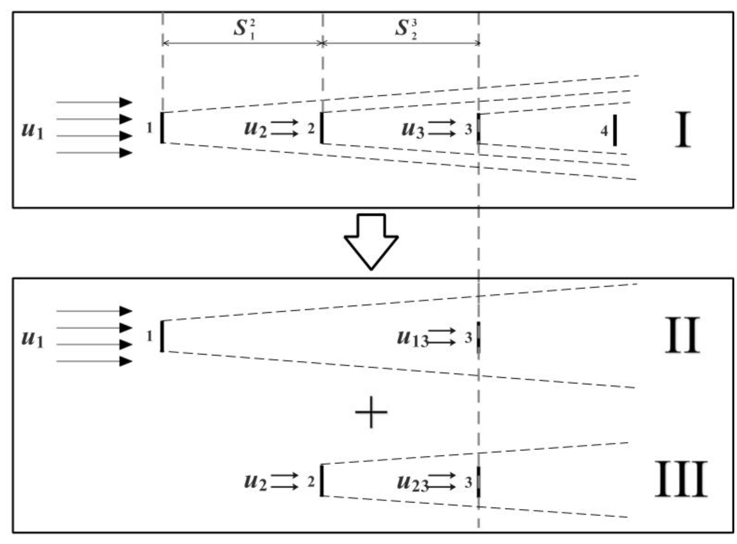
Except for the GS model, all models first calculate the wake losses of each upwind turbine at the position of the target turbine and then overlay them as the total loss due to upwind turbines. Hence, the only distinction between the superposition models is that the wake deficit is expressed in different ways. Figure 1 gives a schematic for the typical wake superposition along a row of four turbines. As shown, wind turbine 3 is located in the superimposed zone of upwind turbines 1 and 2. When calculating the velocity distribution before turbine 3 in scenario I, first, the superposition should be divided into scenario II and scenario III. Then, the wake deficits caused by turbines 1 and 2 are computed separately and finally combined as the total loss caused by upwind turbine.
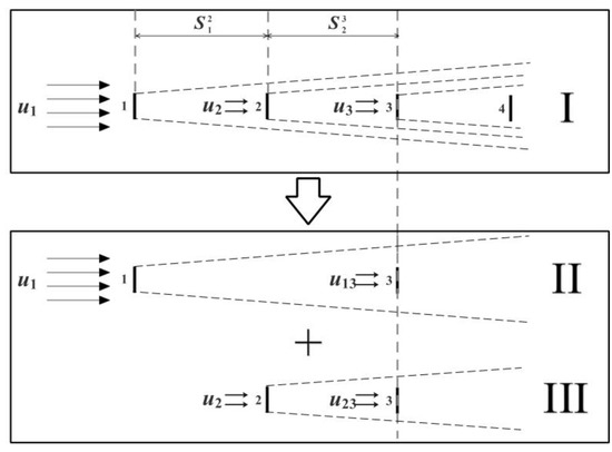
Figure 1.
Schematic diagram of three overlapping turbine wakes. The simulation of the inflow velocity at turbine 3 in scenario I is decomposed into scenarios II and III, and then superimposed.
In the far wake region, turbulence plays a leading role in the flow development. The turbulent environment re-energises the low-momentum wake regions within wind farms [32]. The wind speed gradient between the wake and the free flow outside the wake results in additional shear-generated turbulence, which assists the transfer of momentum into the wake from the surrounding flow. Thus the wake and the surrounding flow start to mix. The rate of decay of the velocity deficit is strongly dependent on the ambient turbulence levels [33,34]. As a general rule of thumb [35,36], the stronger the ambient turbulent intensity, the faster the wake recovery. Some wind tunnel experiments and CFD simulations [37,38] have shown that the turbulence intensity in the wake overlay area is higher than that of the undisturbed wind turbine at the same location. Meanwhile, as mentioned above, for a particular experiment of two turbines in a row, the wake velocity of the downwind turbine recovers more rapidly than that of the upwind one. So this can be explained by the fact that the turbulence level generated by the upwind turbines is higher, which creates more momentum diffusion, leading to a faster recovery in the superposed area. Traditional interaction models are merely the mathematical expressions of the wake losses and simple superimposition. They cannot take account of the effect induced by the increased turbulence intensity. To overcome this limitation, this study multiplies the superimposed total loss—i.e., terms at the right of equal-sign in the traditional models—by a mixing coefficient less than 1 to characterize the faster velocity recovery caused by an increased turbulence intensity in the superposed wake area. The mixing coefficient can be described by an empirical formula as follows:
where refers to the spacing between every two upwind adjacent turbines along the wind direction as shown in Figure 1; dT is the rotor diameter; and Save is their average value.
The mixing coefficient can be calculated fast using Equations (2) which is only based on the spacing between upwind turbines. This expression meets two requirements: First, the coefficient is always less than 1 characterizing less total loss in the wake overlay area due to the higher turbulence level. Second, according to some experimental results [39,40], smaller upwind turbine spacing could lead to larger turbulence intensity in the superimposed area. So the mixing coefficient tends to be smaller with denser upwind turbines, which means faster velocity recovery.
With the exception of the EB model, all traditional interaction models are empirical descriptions without a clear physical basis. With this in mind, the mixing coefficient is combined with the EB model, and then the modified energy balance model (MEB for short) is proposed as follows:
Having a similar form to the EB model, the MEB model can be used with ease and no additional complexity is added to the flow field calculation. However, it should be noted that this modification is appropriate only if there are large perturbations in the wake superposition, such as an array of wind turbines along the wind direction. When considering the superposition of two wakes abreast, the relative spacing along the wind direction between the two turbines is 0, so the mixing coefficient which is based on this spacing cannot be solved and the MEB model does not apply. For this case the traditional EB model is recommended to predict the velocity deficit in the interference region.
2.3. Relative Position of Wind Turbines under Arbitrary Directions
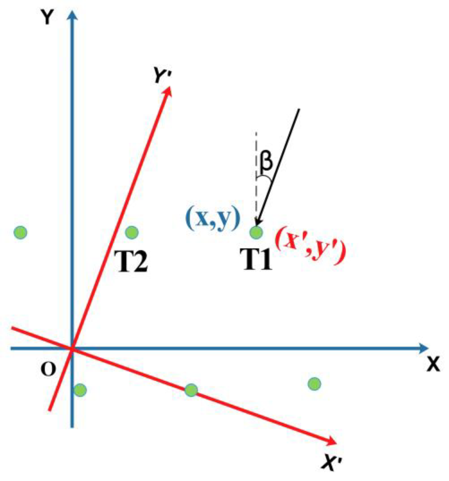
When the wind direction changes, the wind turbine conducts yaw control to ensure that the rotor swept plane is always perpendicular to the inflow direction, which changes the relative positions of the turbines and the wake effect. Therefore, determining the relative position of wind turbines efficiently under arbitrary wind direction is a required process for predicting wake deficits [41]. We use a simple method to solve this problem in this research. As shown in Figure 2, north is regarded as 0° and has the established coordinate frame XOY. The coordinate origin can be chosen from any point in the wind farm, and the Y axis points to the 0° wind direction. T1 represents an arbitrary wind turbine with position (x, y). When the wind direction changes to β, the coordinates are rotated β degrees clockwise and a new coordinate system X’OY’ is obtained. The coordinates of the wind turbine in frame X’OY’ can be obtained by:

Figure 2.
Schematic representation of the coordinate transformation. Green points represent wind turbines.
After the coordinate transformation, the relative positions of the wind turbines can be determined. Combining with the single wake model and the above-mentioned interaction wake model, the wake velocity distribution and power output can be obtained for varying wind directions in wind farm.
3. Benchmarking Study
3.1. Lillgrund Wind Farm
3.1.1. Introduction
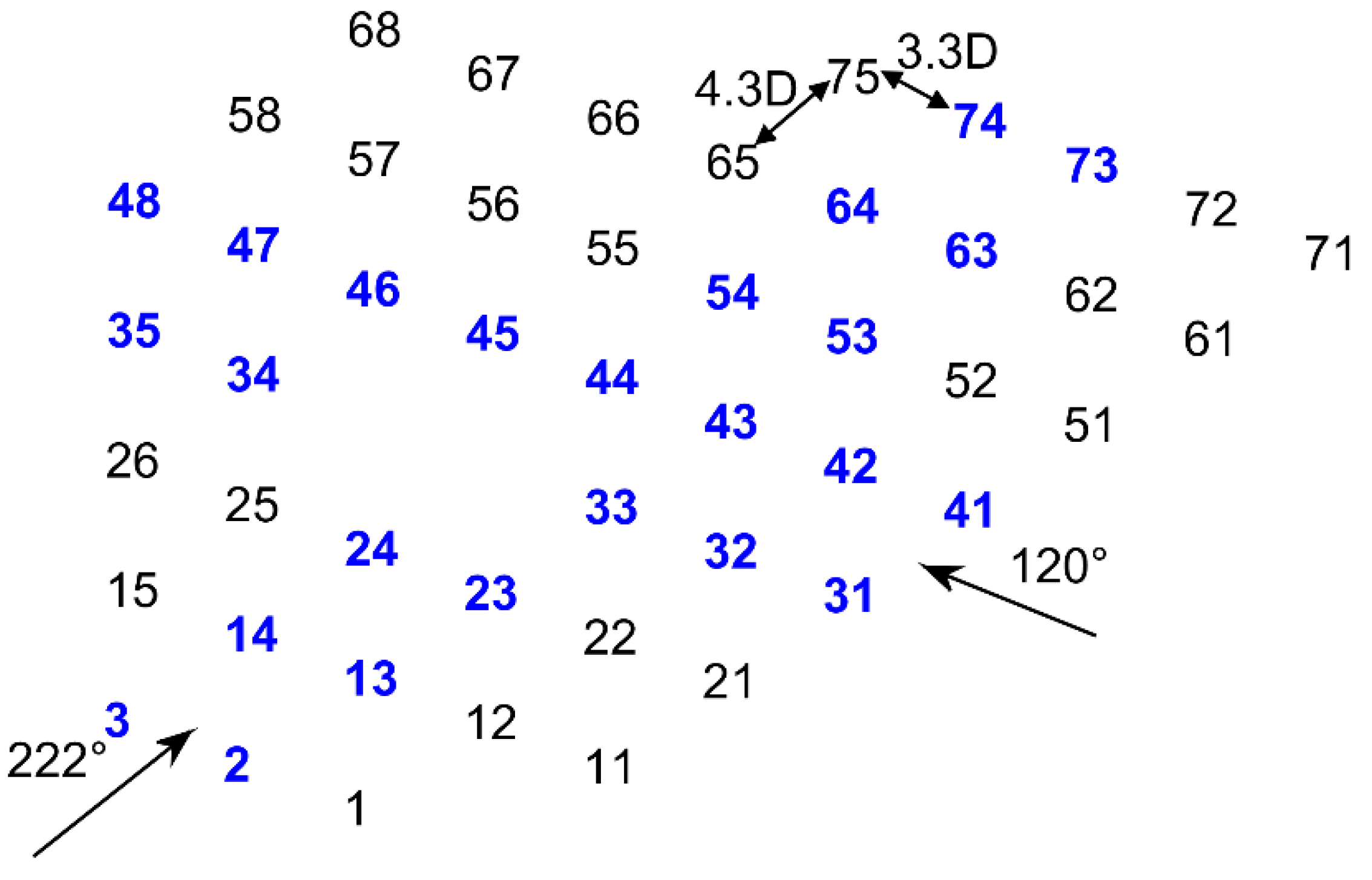
The Lillgrund wind farm consists of 48 SWT-2.3-93 Simens wind turbines with a wind rotor diameter of 92.6 m and hub height of 65 m. Since the typical characteristic of this park is that the internal spacing between adjacent turbines is relatively small, the power loss due to the wake effect is bound to be very large. Figure 3 gives the layout of the Lillgrund offshore wind farm. As shown, the turbine spacing is 3.3D and 4.3D rotor diameters under the wind direction of 120° and 222°, respectively.

Figure 3.
Layout of the Lillgrund offshore wind farm.
3.1.2. Results and Discussion
The co-axial arrangement of wind turbines can be observed in the above two directions. In order to test the accuracy of different models, the Jensen model is combined with three previous interaction wake models (LS, EB, SS) and with the proposed MEB model to calculate the power deficit along rows with and without missing turbines (in blue in Figure 3). The inflow mean velocity at hub height is 9 m/s in all cases. The wake expansion rate of the Jensen model is set to be 0.05 according to the recommended value for offshore conditions. The calculations are performed for various wind directions, consistent with those of the inflow sector of processed SCADA (Supervisory Control and Data Acquisition System) data [−2.5°,2.5°] [11], and are performed in 0.5° steps for both arrays in this research. The results for these cases are given in Figure 4 and Figure 5. The power deficit of the wind turbine can be defined as , where is the actual power of a specific turbine i and is the power of a turbine not disturbed by a wake.
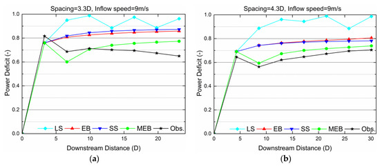
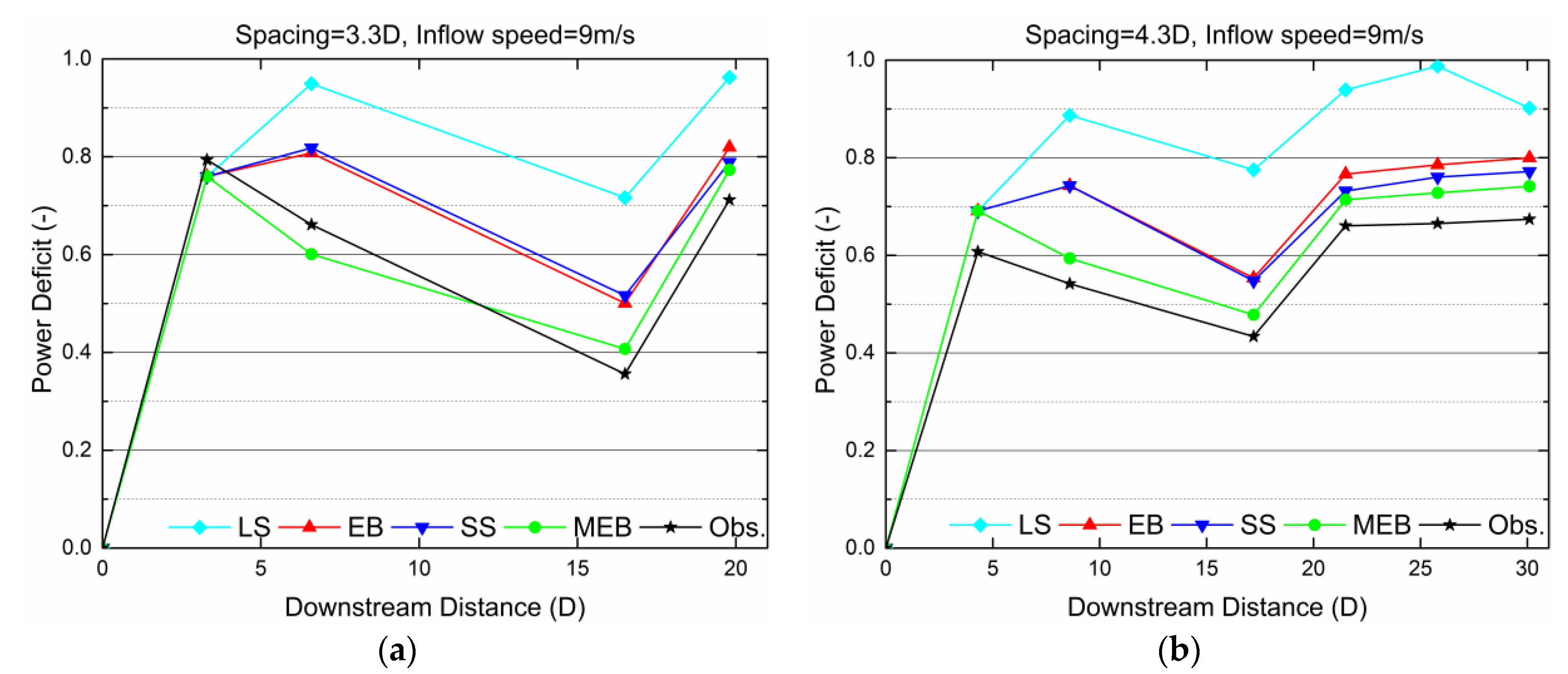
Figure 4.
Lillgrund power deficit in a complete row with (a) 3.3D spacing and (b) 4.3D spacing.
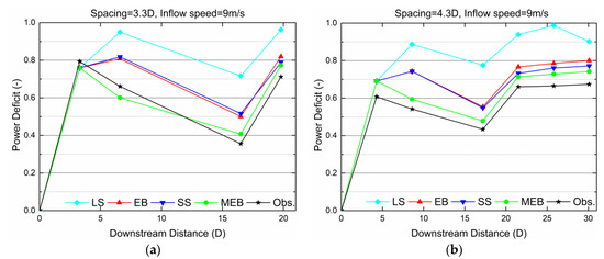
Figure 5.
Lillgrund power deficit in a row with (a) 3.3D spacing with two missing turbines and (b) 4.3D spacing with one missing turbine.
Figure 4 shows the variation of power deficit for different turbine separation distances in the complete arrays along the two directions. In these two cases, the results from the EB model and SS model are very similar, while the LS model seriously over-predicts the deficit and presents a zig-zag pattern. This is because when the calculated inflow is less than the rated speed of the wind turbine, the turbine will stop operating, and no wake is produced in this study. Specifically, without a superposition effect, the power deficits of the second turbine predicted by different models are the same and reach up to about 82% and 65%, respectively, because of the small spacing. As for the third turbine, the power deficit significantly decreases compared with the former one. Neither of the three typical models could capture this trend, but show rather a continuous decrease of power. Only the proposed MEB model perfectly predicts the power recovery of the third turbine. For the case with 4.3D spacing, the MEB model simulation results of the fourth and subsequent turbines agree very well with observations. However, what should be noted is that none of the superposition models predict the trend of power recovery after the third turbine for the case of 3.3D spacing. Perhaps this is because of the error in the single wake model due to the overly close spacing of 3.3D. Katic [17] also admitted that the calculation of the near-wake zone will involve large errors using the Jensen wake model.
The input data and the characteristics of the cases shown in Figure 5 are more or less the same as in the previous ones, except that some turbines are missing in the studied rows. The absence of turbines causes wakes to further recover to some extent from the third turbine to the fourth. The traditional model results also show this pattern, simply because a smaller predicted inflow before the third turbine leads to a lower overall velocity deficit (the right hand of the model equation) and so a higher inflow before the fourth turbine in the calculation. The MEB model proposed in this study not only catches the sustained power recovery of turbines three and four, but also agrees with the measurements better than the other models in both cases.
In addition to power deficit, the efficiency of the wind farm is another performance indicator measuring the precision of the interaction wake model, which is defined as the ratio between the wind farm actual total output power and the power of the wind farm without considering the wake effect for each turbine. The efficiency can be expressed as:
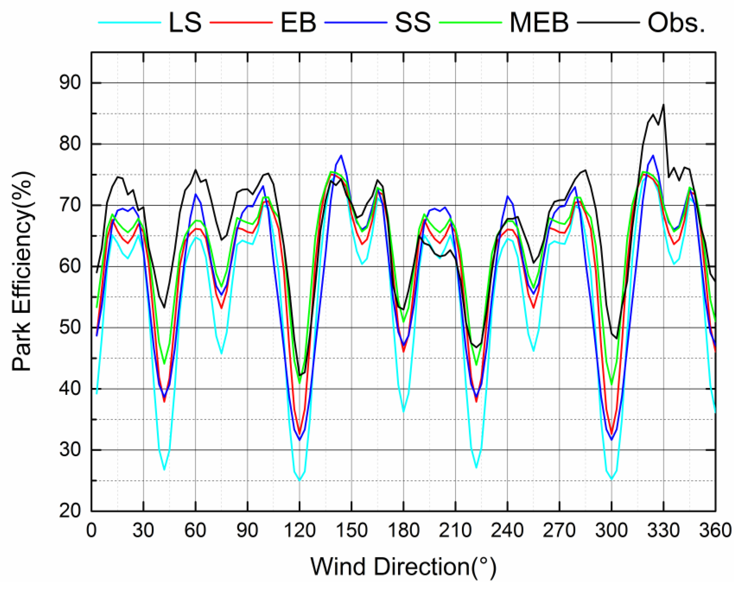
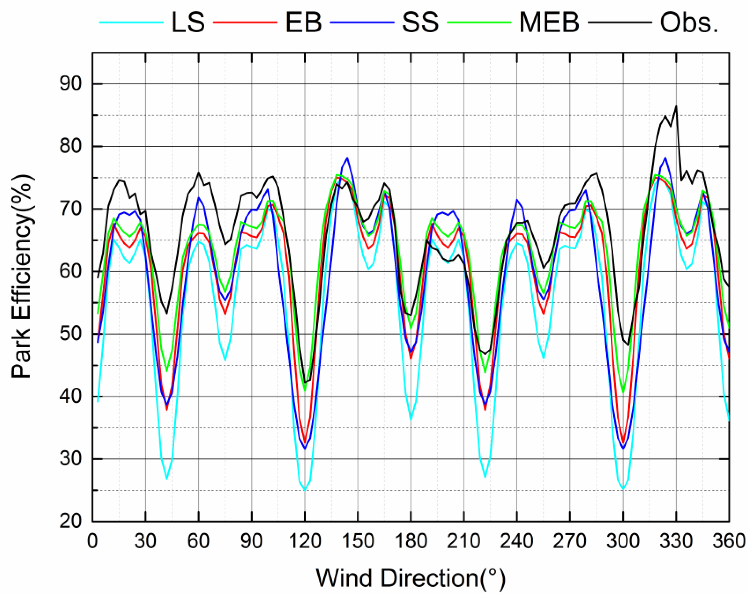
where M is the number of wind turbines in the wind farm. The Jensen model is integrated with four superposition models to calculate the park efficiency under all the wind directions with a span of 3°. In every direction, the inflow mean velocity is 9 m/s. Comparisons of the simulation results with field measurements are given in Figure 6. In general, all the four models could broadly predict the variation of efficiency with changing wind direction and the location of the extreme points. However, there still exist some biases between the model results and observations, especially for the LS model.
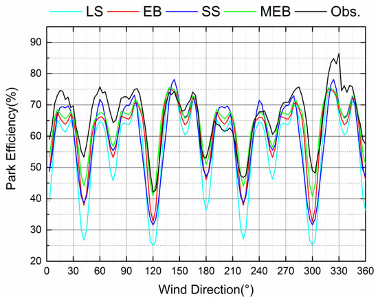
Figure 6.
Park efficiency of the Lillgrund wind farm for the inflow sector 0–360° with 3° increments.
To conduct quantitative analysis, the root mean square error (RMSE) and the mean absolute percentage error (MAPE) are adopted to measure the difference between predictions and observations and to evaluate the model performance. Their definitions are as follows:
where K is the total number of simulated cases in different wind directions; effmodel,i and effobs,i refer to the efficiency from the model prediction and field measurement of the ith given wind direction. The RMSE and MAPE of different model simulation results are listed in Table 1, and the error of models under prevailing wind direction sectors (240°–270°) is also shown. It can be seen that under the inflow sector (0–360°), the park efficiency calculated by the MEB model reduces the RMSE by 3.79% and decreases the MAPE by 5.3% in comparison to the most commonly used SS model. Moreover, these values are reduced by 1.96% and 2.48%, respectively, in the dominant wind direction range.

Table 1.
Simulation error of the park efficiency using different models.
3.2. Horns Rev I Wind Farm
3.2.1. Introduction
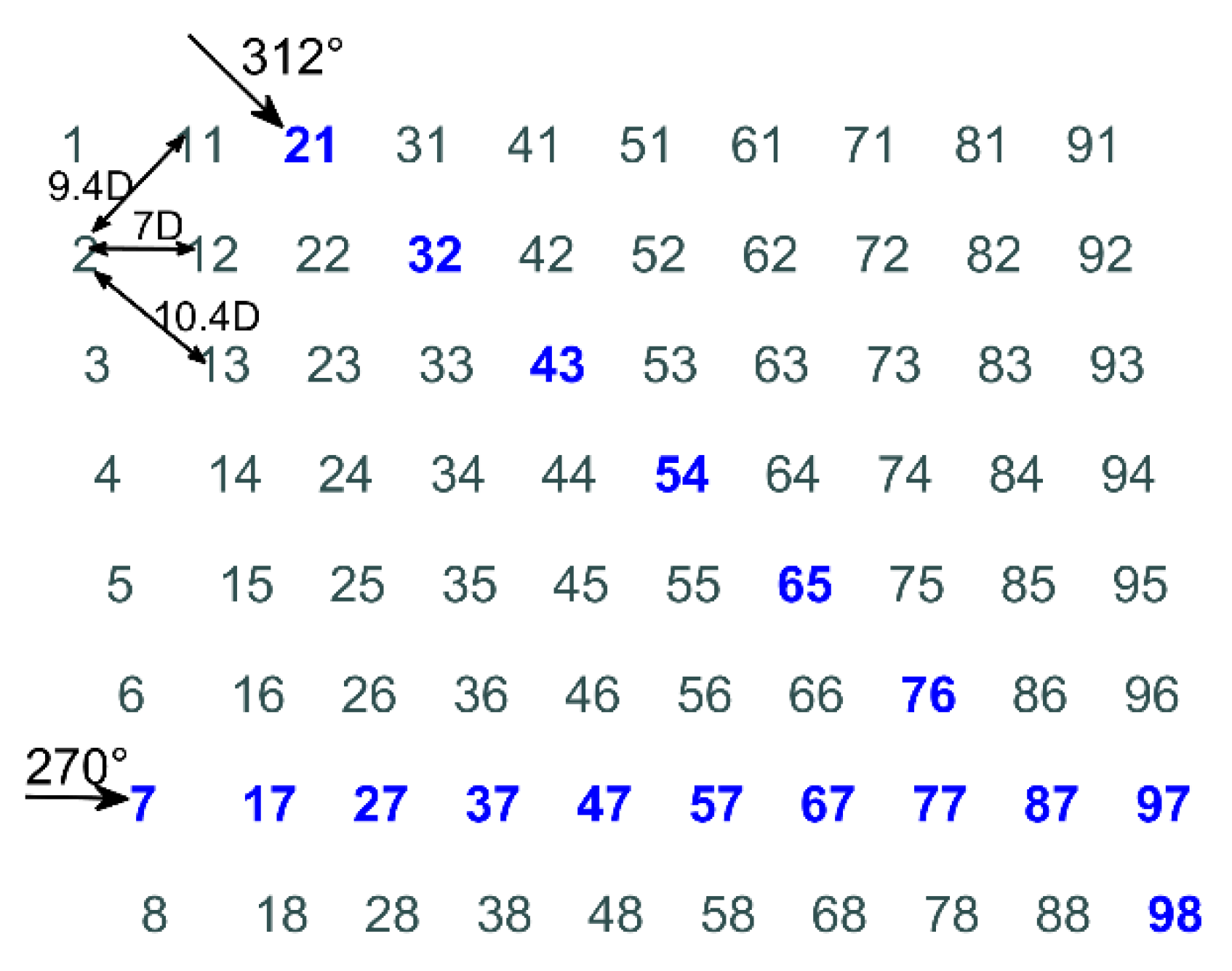
The Horns Rev I offshore wind farm is located about 14 km off the west coast of Denmark. It has been extensively studied in evaluating its wake effect and power production, with plenty of meteorological and SCADA data available for comparison. The wind farm consists of 80 Vestas V80 2 MW turbines with a rotor diameter of 80 m and hub height of 70 m. The wind farm’s 10 columns and 8 rows are aligned in a parallelogram shape, as seen in Figure 7. The spacing distance between turbines in both lines and columns is 7D, and those under the wind direction of 221° and 312° are 9.4D and 10.4D, respectively.
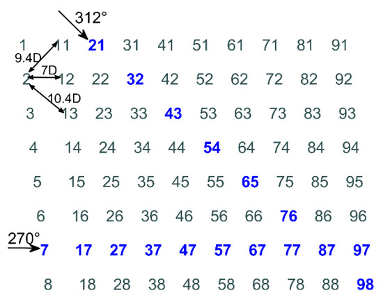
Figure 7.
Layout of the Horns Rev I offshore wind farm.
3.2.2. Results and Discussion
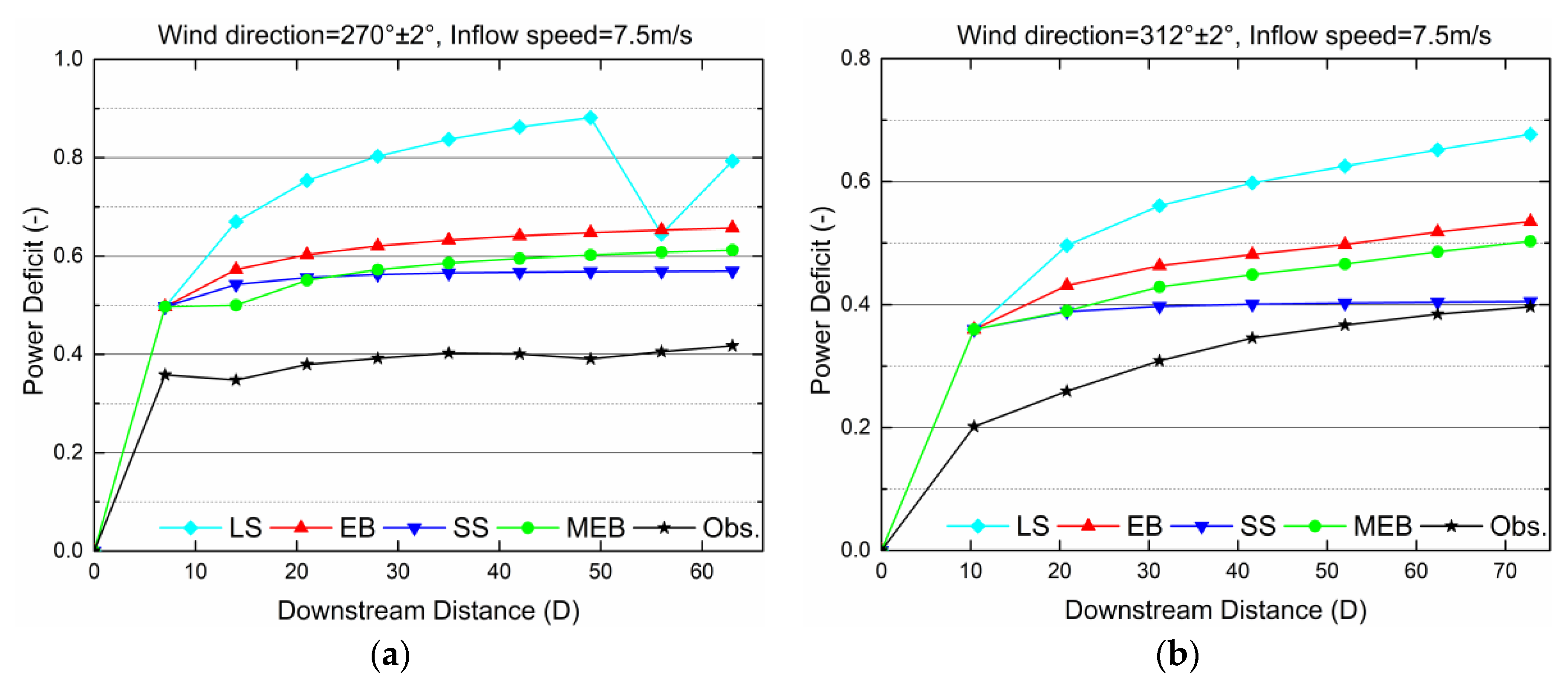
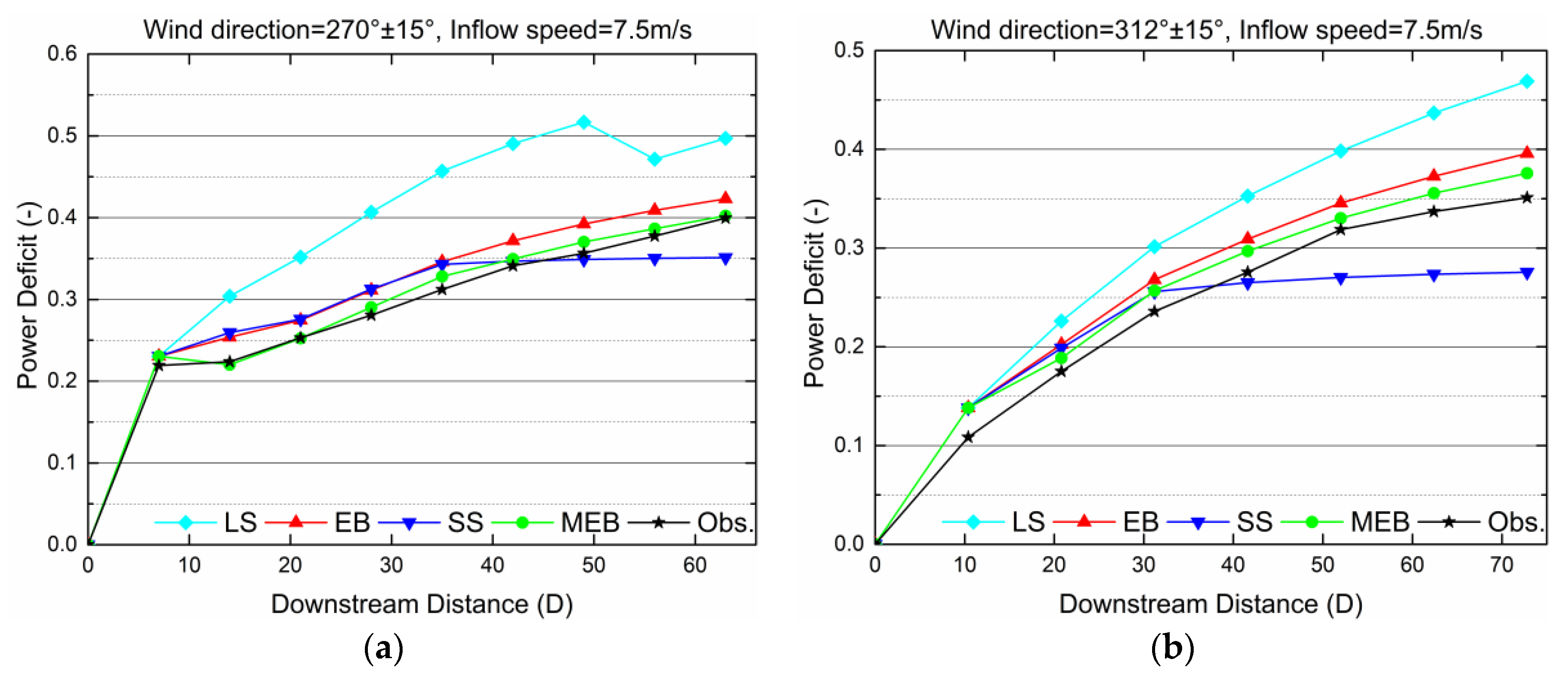
The Jensen model is also chosen in this benchmark with k = 0.05. Four different interaction models are applied to predict the power deficit of each turbine along rows with an internal spacing of 7D and 10.4D, respectively (in blue in Figure 7). The comparisons between simulation results obtained from different models and extracted SCADA data [22] with an inflow velocity of 7.5 m/s are given in Figure 8 and Figure 9. The cases in Figure 8 correspond to narrow wind direction sizes [−2°,2°], and the cases in Figure 9 correspond to a broader direction interval [−15°,15°], which is considered to decrease the error of wind direction uncertainty as much as possible. All of the runs were performed at a 1° step.
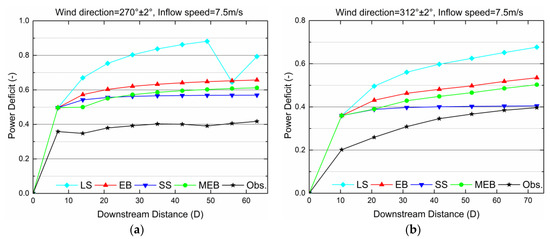
Figure 8.
Horns Rev I power deficit in (a) a row with 7D spacing and 270 ± 2°, and (b) a row with 10.4D spacing and 312 ± 2°.
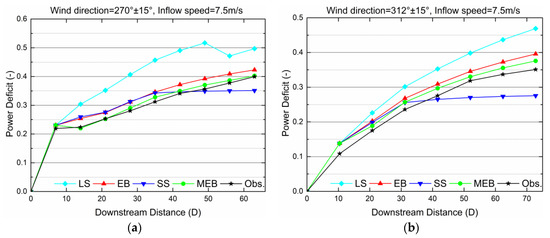
Figure 9.
Horns Rev I power deficit in (a) a row with 7D spacing and 270 ± 15°, and (b) a row with 10.4D spacing and 312 ± 15°.
When the wind directions are 270° and 312°, the spacing between two turbines undergoes a minimum value of 7D and a maximum value of 10.4D, respectively. Observing the power deficit of the second turbine in Figure 8, there is a large discrepancy when comparing numerical simulations using the Jensen model with wind farm production data. In addition to the reasons for the calculation accuracy of the wake model itself, another important reason is the large wind direction uncertainty included in the datasets while the numerical simulations are carried out for narrow wind direction sectors. Thus, when comparing the performance of different wake interaction models, the primary concern is whether the simulation results can match the changing trend of the measured data. It can be seen from Figure 8a that, with an internal spacing of 7D, the power of the third turbine has recovered more or less compared with the second one. After that, the power deficit tends to gradually increase with a very small range further downwind until the last turbine. The improved MEB model simulation catches the recovery of the power of the third turbine, and the power deficit of the latter turbines increases gradually with a slightly greater amplitude than the measured value. On the other hand, the simulation results of the SS model tend to be in an equilibrium value starting from the third turbine. When the spacing is 10.4D, the power deficit caused by the wake is relatively small due to the larger interval between turbines, and it can be clearly seen from Figure 8b that the deficit along the wind direction increases in steps. At this time, the SS model calculation result, which reach a constant, are obviously inconsistent with the changing trend of the measured values, although the calculated downwind turbine power is closer to the measured value. The power deficit variation curves simulated by the new MEB model and the EB model more closely match the observed values. In fact, the results of the MEB and EB model show the similar changing trend after the third turbine. This is because the MEB model just multiplies a coefficient to the original EB model. In essence, the mathematical structure of these two models is consistent.
With a broader sector [−15°,15°], the comparisons in Figure 9 show that the Jensen model coupled with interaction models matches much better with all the measured points due to the smaller direction uncertainty error, especially for the new MEB and EB models. The LS model still seriously overestimates the wake loss in the superposition region, while the SS model fails to model the deep array effect as it quickly reaches an equilibrium state. Note that, with the internal spacing of 7D, as seen in Figure 9a, the power of the third turbine restores compared to the second one simulated by the MEB model; nevertheless, the measurements show a slight decrease. This departure may be due to the different frequency of wind directions within the sector [−15°,15°]. The authors in Reference [24] pointed out that a normal distribution fits well with the measured wind direction variations within an averaging period at Horns Rev I around the wind direction of 270°. That is to say, there are a greater number of available measurements for data analysis near 270°, and the number of measurements which are close to the wind direction interval boundary are relatively small. Thus, data for directions near 270°, of which the wake losses of downwind turbines are much heavier, contribute more to the final processing results. However, simulations in this study are performed for a wide range of wind directions (±15°) with a resolution of 1°. These single simulated powers are then averaged within the range. Therefore, the effect of the cases under directions further away from 270° is overestimated, which results in less deficit in the turbines. In addition, since the turbines are far apart from each other, the upwind wake has restored to a certain degree when it develops to the downwind turbine. The turbulence intensity in the far wake superimposed area tends to be similar to the single wake, which leads to the calculation results of the MEB model and EB being relatively close, as shown in Figure 9b. The farther the spacing, the closer the mixing coefficient is to 1, and so the closer the calculation result of the new model is to the EB model.
Similar models as in the previous benchmark are considered to calculate the park efficiency, and the inflow sector is taken as 0–360° with a span of 5°. In every direction, the inflow mean velocity is 8 m/s. The comparison of the simulation results with measurements is shown in Figure 10. There are significant differences in some wind directions where the wake has a large impact, such as for 0° and 270°. The RMSE and MAPE of different model simulation results are listed in Table 2. It can be seen that under the inflow sector (0–360°), compared with the SS model, the MEB model reduces the wind farm efficiency RMSE by 1.39% and MAPE by 1.58%. Under the dominant wind direction, the wind farm efficiency RMSE decreased by 1.79%, and the MAPE decreased by 2.52%. The results show that for wind farms such as Horns Rev I, which conducts reasonable layout optimization and has a relatively large spacing distance between turbines, the performance of the MEB model has a certain degree of improvement compared with the EB and SS model. However, this improvement is not as good for the Lillgrund wind farm with smaller intervals between turbines.
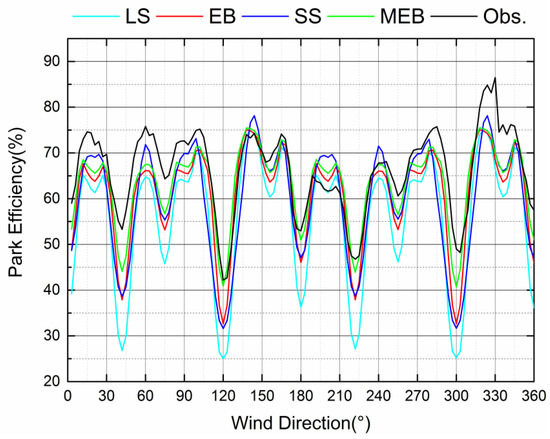
Figure 10.
Park efficiency of the Horns Rev I wind farm for inflow sector 0–360° with a 5° increment.

Table 2.
Simulation error of park efficiency using different models.
4. Conclusions
The conventional interaction wake models separately compute the velocity deficit from each upwind turbine and then linearly superpose them without considering the faster wake recovery caused by a higher turbulence intensity in the superposed wake region, when compared to a single wake area. This omission might contribute to lower model precision. To compensate for this, a new interaction wake model based on the improvement of the energy balance model is proposed to predict the velocity distribution and wind farm power in this paper. A mixing coefficient is introduced to characterize the above phenomenon in the energy balance model, and an empirical expression is also given to calculate this parameter. In order efficiently to provide support for simulating the wake speed distribution under varying wind directions, a simple method to determine the relative position between wind turbines is also given.
A validation of the proposed interaction model is performed using the observations in the Lillgrund and Horns Rev I offshore wind farms, mainly focusing on the power loss of every single turbine and the efficiency of the wind farms. Compared to other commonly used superposition models in engineering, the presented model can better capture the power changing tendency of wind turbines arranged in an array with different spacing, regardless of whether there are missing turbines or not. Especially for turbines in a row in the Lillgrund offshore wind farm with smaller turbine spacing, an obvious power recovery appears at the third turbine, which is only predicted by the presented model. As for the wind farm efficiency, all the interaction models can obtain the changing trend of wind farm output with varying wind direction and determine the location of limit points, while the proposed model in particular is observed to be in better agreement with the measurements.
The proposed interaction model has similar simplicity but higher precision compared with the commonly used interaction models, without increasing the complexity and computational cost of the simulation because the former only multiplies the traditional one by a mixing coefficient. This coefficient is used to characterize the phenomenon that the higher turbulence level and shear stress profile generated by upwind turbines in the superposed wake area leads to a faster wake recovery, which is obtained by an empirical expression in this paper. Although the modification yields reasonable predictions, a more physical and more accurate model describing the effect of turbulence intensity on the velocity recovery of multiple wakes will be the focus of future research.
Author Contributions
The paper was a collaborative effort among the authors. Z.S. performed the modeling, analyzed the data, and wrote the paper. Y.L. supervised the related research work. L.L. and S.H. contributed analysis tools. Y.W. polished the language.
Funding
This research was funded by the National Key Research and Development Program of China (No. 2017YFE0109000), and Open Fund of Operation and Control of Renewable Energy & Storage Systems (No. 1810-00895).
Acknowledgments
Thanks to the support by the National Key Research and Development Program of China (No. 2017YFE0109000), and Open Fund of Operation and Control of Renewable Energy & Storage Systems (No. 1810-00895).
Conflicts of Interest
The authors declare no conflict of interest.
References
- Barthelmie, R.J.; Rathmann, O.; Frandsen, S.T.; Hansen, K.; Politis, E.; Prospathopoulos, J.; Rados, K.; Cabezón, D.; Schlez, W.; Phillips, J.; et al. Modelling and measuring flow and wind turbine wakes in large wind farms offshore. Wind Energy 2009, 12, 431–444. [Google Scholar] [CrossRef]
- Wang, Y.; Liu, Y.; Li, L.; Infield, D.; Han, S. Short-term wind power forecasting based on clustering pre-calculated CFD method. Energies 2018, 11, 854. [Google Scholar] [CrossRef]
- Tian, J.; Zhou, D.; Su, C.; Soltani, M.; Chen, Z.; Blaabjerg, F. Wind turbine power curve design for optimal power generation in wind farms considering wake effect. Energies 2017, 10, 395. [Google Scholar] [CrossRef]
- Herbert-Acero, J.F.; Probst, O.; Réthoré, P.E.; Larsen, G.C.; Castillo-Villar, K.K. A review of methodological approaches for the design and optimization of wind farms. Energies 2014, 7, 6930–7016. [Google Scholar] [CrossRef]
- Peña, A.; Rathmann, O. Atmospheric stability-dependent infinite wind-farm models and the wake-decay coefficient. Wind Energy 2014, 17, 1269–1285. [Google Scholar] [CrossRef]
- Ferrer, E.; Browne, O.M.F.; Valero, E. Sensitivity Analysis to Control the Far-Wake Unsteadiness behind Turbines. Energies 2017, 10, 1599. [Google Scholar] [CrossRef]
- Munters, W.; Meyers, J. Dynamic strategies for yaw and induction control of wind farms based on large-eddy simulation and optimization. Energies 2018, 11, 177. [Google Scholar] [CrossRef]
- Renkema, D.J. Validation of Wind Turbine Wake Models. Master’s Thesis, Delft University of Technology, Delft, Holland, 2007. [Google Scholar]
- Niayifar, A.; Porté-Agel, F. Analytical modeling of wind farms: A new approach for power prediction. Energies 2016, 9, 741. [Google Scholar] [CrossRef]
- Jeon, S.; Kim, B.; Huh, J. Comparison and verification of wake models in an onshore wind farm considering single wake condition of the 2MW wind turbine. Energy 2015, 93, 1769–1777. [Google Scholar] [CrossRef]
- Göçmen, T.; Laan, P.V.D.; Réthoré, P.E.; Diaz, A.P.; Larsen, G.C.; Ott, S. Wind turbine wake models developed at the technical university of Denmark: A review. Renew. Sust. Energy Rev. 2016, 60, 752–769. [Google Scholar] [CrossRef]
- Hasager, C.B.; Rasmussen, L.; Peña, A.; Jensen, L.E.; Réthoré, P.-E. Wind farm wake: The Horns Rev photo case. Energies 2013, 6, 696–716. [Google Scholar] [CrossRef]
- Van Leuven, J. The Energetic Effectiveness of a Cluster of Wind Turbines. Master’s Thesis, Universite Catholique de Louvain, Louvain-la-Neuve, Belgium, 1992. [Google Scholar]
- Lissaman, P.B.S. Energy effectiveness of arbitrary arrays of wind turbines. J. Energy 1979, 3, 323–328. [Google Scholar] [CrossRef]
- Crespo, A.; Hernández, J.; Frandsen, S. Survey of modelling methods for wind turbine wakes and wind farms. Wind Energy 1999, 2, 1–24. [Google Scholar] [CrossRef]
- Crespo, A.; Manuel, F.; Hernández, J. Numerical modelling of wind turbine wakes. In Proceedings of the 1990 European Community Wind Energy Conf., Madrid, Spain, 8–12 March 1990; pp. 66–170. [Google Scholar]
- Katic, I.; Højstrup, J.; Jensen, N.O. A simple model for cluster efficiency. In Proceedings of the European Wind Energy Association Conference & Exhibition, Rome, Italy, 7–9 October 1986; pp. 407–410. [Google Scholar]
- Rados, K.G.; Voutsinas, S.G.; Zervos, A. Wake effects in wind parks. A new modelling approach. In Scientific Proceedings; EWEC: Travemunde, Germany, 1993; pp. 444–447. [Google Scholar]
- Erik, D. Evaluation of the Software Program Windfarm and Comparisons with Measured Data from Alsvik. Master’s Thesis, Royal Institute of Technology, Stockholm, Sweden, 2000. [Google Scholar]
- Tian, L.L.; Zhu, W.J.; Shen, W.Z.; Yong, Y.L.; Zhao, N. Prediction of multi-wake problems using an improved Jensen wake model. Renew. Energy 2017, 102, 457–469. [Google Scholar] [CrossRef]
- Jensen, N.O. A Note on Wind Generator Interaction; Technical Report Risoe-M-2411(EN); Risø National Laboratory: Roskilde, Denmark, 1983. [Google Scholar]
- VanLuvanee, D.R. Investigation of Observed and Modeled Wake Effects at Horns Rev Using WindPRO. Master’s Thesis, Technical University of Denmark, Copenhagen, Denmark, 2006. [Google Scholar]
- Peña, A.; Réthoré, P.E.; Hasager, C.B.; Hansen, K.S. Results of Wake Simulations at the Horns Rev I and Lillgrund Wind Farms Using the Modified Park Model; DTU Wind Energy-E-Report-0026(EN); Risø Campus: Roskilde, Denmark, 2013. [Google Scholar]
- Gaumond, M.; Rethoré, P.E.; Ott, S.; Peña, A.; Bechmann, A.; Hansen, K.S. Evaluation of the wind direction uncertainty and its impact on wake modelling at the Horns Rev offshore wind farm. Wind Energy 2014, 17, 1169–1178. [Google Scholar] [CrossRef]
- Gao, X.X.; Yang, H.X.; Lu, L. Optimization of wind turbine layout position in a wind farm using a newly-developed two-dimensional wake model. Appl. Energy 2016, 174, 192–200. [Google Scholar] [CrossRef]
- Mortensen, N.G.; Heathfield, D.N.; Myllerup, L.; Landberg, L.; Rathmann, O. Getting Started with WAsP 9; Technical Report Risø-I-2571(EN); Risø National Laboratory: Roskilde, Denmark, 2007. [Google Scholar]
- Thørgersen, M.; Sørensen, T.; Nielsen, P.; Grötzner, A.; Chun, S. WindPRO/PARK: Introduction to Wind Turbine Wake Modelling and Wake Generated Turbulence; EMD International A/S: Aalborg, Denmark, 2005. [Google Scholar]
- Kuo, J.Y.J.; Romero, D.A.; Amon, C.H. A mechanistic semi-empirical wake interaction model for wind farm layout optimization. Energy 2015, 93, 2157–2165. [Google Scholar] [CrossRef]
- Smith, D.; Taylor, G.J. Further analysis of turbine wake development and interaction data. In Proceedings of the 13th BWEA Wind Energy Conf., Swansea, Wales, 20–26 October 1991; pp. 325–331. [Google Scholar]
- Frandsen, S. On the wind speed reduction in the center of large clusters of wind turbines. J Wind Eng. Ind. Aerod. 1992, 39, 251–265. [Google Scholar] [CrossRef]
- Peña, A.; Réthoré, P.-E.; van der Laan, M.P. On the application of the Jensen wake model using a turbulence-dependent wake decay coefficient: The Sexbierum case. Wind Energy 2016, 19, 763–776. [Google Scholar] [CrossRef]
- Tobin, N.; Chamorro, L.P. Modulation of turbulence scales passing through the rotor of a wind turbine. J. Turbul. 2018, 1–11. [Google Scholar] [CrossRef]
- Burton, T.; Sharpe, D.; Jenkins, N.; Bossanyi, E. Wind Energy Handbook; John Wiley & Sons Ltd.: Chichester, UK, 2001; pp. 35–37. ISBN 0-471-48997-2. [Google Scholar]
- Makridis, A. Modelling of Wind Turbine Wakes in Complex Terrain Using Computational Fluid Dynamics. Master’s Thesis, the University of Edinburgh, Edinburgh, UK, 2012. [Google Scholar]
- Crespo, A.; Herna´ndez, J. Turbulence characteristics in wind-turbine wakes. J. Wind Eng. Ind. Aerod. 1996, 61, 71–85. [Google Scholar] [CrossRef]
- Duckworth, A.; Barthelmie, R.J. Investigation and validation of wind turbine wake models. Wind Eng. 2008, 32, 459–475. [Google Scholar] [CrossRef]
- Veisi, A.A.; Shafiei Mayam, M.H. Effects of blade rotation direction in the wake region of two in-line turbines using Large Eddy Simulation. Appl. Energy 2017, 197, 375–392. [Google Scholar] [CrossRef]
- Lee, S.; Vorobieff, P.; Poroseva, S. Interaction of Wind Turbine Wakes under Various Atmospheric Conditions. Energies 2018, 11, 1442. [Google Scholar] [CrossRef]
- Liu, H.; Hayat, I.; Jin, Y.; Chamorro, L.P. On the evolution of the integral time scale within wind farms. Energies 2018, 11, 93. [Google Scholar] [CrossRef]
- Chamorro, L.P.; Porté-Agel, F. Turbulent flow inside and above a wind farm: A wind-tunnel study. Energies 2011, 4, 1916–1936. [Google Scholar] [CrossRef]
- Gu, B.; Liu, Y.; Yan, J.; Li, L.; Kang, S. A wind farm optimal control algorithm based on wake fast-calculation model. J. Sol. Energy Eng. 2016, 138, 024501:1–024501:6. [Google Scholar] [CrossRef]
© 2019 by the authors. Licensee MDPI, Basel, Switzerland. This article is an open access article distributed under the terms and conditions of the Creative Commons Attribution (CC BY) license (http://creativecommons.org/licenses/by/4.0/).

