An Optimized Impedance Model for the Estimation of the State-of-Charge of a Li-Ion Cell: The Case of a LiFePO₄ (ANR26650)

Abstract

This article focused on the estimation of the state of charge (SoC) of a Li-con Cell by carrying out a series of experimental tests at various operating temperatures and SoC. The cell was characterized by electrochemical impedance spectroscopy (EIS) tests, from which the impedance frequency spectrum for different SoC and temperatures was obtained. Indeed, the cell model consisted of a modified Randles circuit type that included a constant phase element so-called Warburg impedance. Each circuit parameter was obtained from the EIS tests. The obtained were been used to develop two numerical models for each parameter, i.e., one based on numerical correlations and the other based on the artificial neural network (ANN) method. A genetic algorithm was used to solve and optimize the numerical models. The accuracy of the models was examined and the results showed that the ANN-based model was more accurate than the correlations-based model. The root mean square relative error (RMSRE) of the parameters Rs, R₁, C₁ and W for the ANN-based model were: 4.63%, 13.65%, 10.96% and 4.4%, respectively, compared to 7.09%, 27.45%, 34.36% and 7.07% for the correlations-based model, respectively. The SoC was estimated using the extended Kalman filter based on a Randles model, with an estimation RMSRE of about 1.19%.

1. Introduction

Lithium-ion batteries are currently considered some of the most efficient devices for energy storage in the medium power capacity range, such as that used in electric vehicles and stationary applications. This is due to their favorable advantages, such as its high power density, long lifetimes, and moderate discharge rate [1]. Nevertheless, the temperature of lithium-ion batteries varies depending on the context in which they are, either increasing or decreasing, thus affecting the performance of the battery. Indeed, the temperature increases during the battery charging and discharging processes.

From the electrical aspect of the batteries it is important to know the state of the battery, which normally includes the state of charge (SoC), state of health (SoH), state of power (SoP) and state of energy (SoE). In general, these states are not observable (i.e., cannot be measured), but need to be estimated from measurements of physical parameters such as voltage, current, temperature or battery usage time.

As future vehicular technologies aim to incorporate high performance batteries, they therefore require an intelligent system to control and monitor the state of the batteries. The current methods used to estimate the states of a battery require a model that represents the physical behavior of the battery. To obtain a good estimate, the model must be accurate, but at the same time simple and cheap.

Electric models vary according to their complexity. In some applications, a simple model that captures the basic electrical behavior of a cell can be used. Electrochemical models are very precise, but are difficult to parametrize and require a high computational capacity [2]. In most applications, equivalent electrical circuits (EECs) are used because they offer a balance between precision and simplicity, and are also useful to obtain an idea of how a cell responds to different usage scenarios. The electrochemical impedance spectroscopy (EIS) method [3] is used to determine the parameters of an equivalent circuit of a battery. The method has a reasonable accuracy when compared to a model with the real-time measurements of the charge/discharge of a battery. However, it does not consider a constant phase element (CPE) to represent the Nyquist diagram of the battery at low frequency.

Considerable efforts have been made by researchers to find more accurate and reliable methods to predict the SoC of a battery. One of the most widely used methods has been the Kalman filter (KF) [4]. The KF estimates the SoC with very low errors and it is easy to implement in real applications. The purpose of the KF is to estimate the state of a system from measurements that contain errors. The original KF is a linear estimation method. To expand its application in non-linear systems, the extended Kalman filter (EKF) [5,6,7,8] and the unscented Kalman filter (UKF) [9,10] have been developed. Both the EKF and UKF methods can estimate the SOC with great accuracy if the battery model is sufficiently accurate and the system is not highly non-linear.

Other methods combine different types of KF. Andre [11], proposed an advanced mathematical method to estimate the SoC and SoH in a lithium-ion battery by combining a standard Kalman filter (KF) and an unscented Kalman filter (UKF). The first filter estimated the polarization overvoltage, the diffusion overvoltage and the ohmic resistance of the equivalent electrical circuit model of the lithium-ion battery. The outputs of the first filter were the inputs for the second filter, which estimated the SoC and the polarization and diffusion resistance. This method was implemented in a code in MATLAB and the simulations indicated an error in the SoC and SoH estimation below 1%. Fengchun et al., in [12] proposed a method to estimate the SoC by considering different health conditions in lithium-ion batteries. The concentrated parameter model was used to model the battery, and was estimated using the square minimum method. A discretization method of the battery model was also proposed, which had the advantage of calibrating the parameters in real time. Subsequently, the parameters were incorporated into the algorithm of the adaptive extended Kalman filter (FKEA) to estimate the SoC. The simulations indicated that the parameters of the battery model degraded as the battery aged, therefore the parameters have to be updated to achieve an optimal performance in the estimation of the battery voltage and the estimation of the SoC. For different levels of battery aging, the error in the SoC estimation was less than 2.5%. Li et al. [13] developed a comparative study of algorithms to estimate the SoC in a LiFePO₄ (LFP) battery used in an electric vehicle. The algorithms that were investigated included the Luenberger observer, extended Kalman filter (EKF) and the sigma Kalman filters or unscented (UKF), which are designed to estimate the SoC in a lithium-ion LFP battery. To evaluate these algorithms, they were verified with two driving profiles typical of an electric vehicle, the new European driving cycle (NECD) and the Artemis cycle. Based on the results of the experimental tests, they concluded that the accuracy of the Luenberger observer was mainly based on the accuracy of the battery model, since it did not take into account the uncertainty of the model and the noise of the measurement. The EKF is comparatively more accurate than the Luenberger observer. Finally, in terms of tracking accuracy, convergence and the robustness of the estimate against the temperature uncertainty and drift current of the sensor, the UKF provided the best results in the SoC estimation unlike the other algorithms.

In recent years, the particle filter (PF) [14,15,16,17,18] has been used to estimate the SoC. Additionally, the PF algorithm is very useful in applications that are considered a non-Gaussian source of uncertainty. The PF requires a considerable number of initial particles and the calculation capacity is very high. In [19], the dependence of the computational load of the PF was solved using a hybrid method to estimate the SoC of a battery based on an adaptive extended Kalman particle filter (AEKPF). Five experimental tests were carried out to evaluate the performance of the algorithm and showed that the average of the absolute error was less than 1%.

The abovementioned methods to estimate the SoC were developed with the model at room temperature, therefore the operation of the method for different temperature conditions of the batteries has not been disclosed, which is important to identify the model parameters for each temperature. The objective of this research was to identify an EEC whose parameters were dependent on the SoC and temperature. In addition, the EEC identification was used to estimate the SoC of a Li-ion cell. The rest of the article is organized as follows: Section 2 presents the electric model of a Li-ion cell, showing that it is necessary to include a constant phase element in the model in relation to the measured data. Section 3 carries out a parametric identification of the EEC for different values of SoC and temperature. For this, an optimization problem was solved by means of a genetic algorithm. In Section 4 a multivariable model was constructed for each EEC parameter based on the SoC and temperature. Two models were tested; in the first, empirical equations were adjusted, while in the second, an ANN was used. In Section 5, the SoC was estimated using the extended Kalman filter algorithm. Finally in Section 6, the conclusions of this research are presented.

2. Electric Model

In this section, an electric model of a Li-ion cell that allowed for the estimation of the electrical behavior is presented. The electrical dynamics are represented by an electric circuit consisting of a voltage source, resistance and a network composed of a capacitor in parallel with a resistor in series with a constant phase element (CPE).

Equivalent Electric Circuit of a Li-ion Cell

The electrical behavior of a battery can be represented by an EEC as shown in Figure 1 [20]. This circuit incorporates a CPE called the Warburg element which accurately reflects the behavior of the cell. The Warburg impedance is a component that produces a partially capacitive and resistive behavior with a phase of 45° at low frequency [21].

Figure 2 shows a Nyquist diagram of a Li-ion cell obtained in the laboratory, where a 45° phase was observed at low frequency. This type of response can be well represented through the circuit shown in Figure 1.

A Warburg element can be expressed in the plane of the frequency in terms of a fractional element as shown in Equation (1):

$${\mathrm{Z}}_{\mathrm{W}}(\mathrm{j}\mathrm{w})=\frac{1}{\mathrm{W}{(\mathrm{j}\mathsf{\omega })}^{\mathsf{\beta }}}$$

(1)

where β $\in$ R, is an arbitrary number 0 ≤ β ≤ 1 [20]; and W $\in$ R is the Warburg coefficient. The phase of the Warburg element in general is βπ/4 [21]. As the phase measured in the laboratory was 45° (π/4), the parameter β was equal to $\frac{1}{2}$.

The input impedance of the electrical circuit in Figure 1 can be defined by Equation (2):

$$\mathrm{Z}={\mathrm{R}}_{\mathrm{s}}+\frac{\frac{1}{\mathrm{j}\mathsf{\omega }{\mathrm{C}}_1}({\mathrm{R}}_1+{\mathrm{Z}}_{\mathrm{W}})}{\frac{1}{\mathrm{j}\mathsf{\omega }{\mathrm{C}}_1}+({\mathrm{R}}_1+{\mathrm{Z}}_{\mathrm{W}})}$$

(2)

The Warburg impedance, defined in Equation (1), indicates that the system has fractional properties, therefore it is necessary to introduce the Fractional Order Calculation (FOC) in the model. The fractional calculation involves derivatives and integrals of a non-integer order, which in the particular case of the Warburg impedance, is determined by the parameter β. The latter is a fractional number [22]. Equation (3) shows the expression of the Warburg impedance voltage in the plane time, which corresponds to a fractional differential equation:

$$\mathrm{W}\frac{{\mathrm{d}}^{\mathsf{\beta }}{\mathrm{v}}_{\mathrm{W}}}{\mathrm{d}{\mathrm{t}}^{\mathsf{\beta }}}={\mathrm{i}}_{\mathrm{W}},$$

(3)

By way of simplification in this paper, we used the notation defined in Equation (4), to express a fractional derivative [21]:

$$\frac{{\mathrm{d}}^{\mathrm{r}}}{\mathrm{d}{\mathrm{t}}^{\mathrm{r}}}={\Delta }^{\mathrm{r}},$$

(4)

where r $\in$ R, is an arbitrary number.

Considering the circuit of Figure 1, the notation defined in Equation (4), and the laws associated with the electric circuits, we can obtain the equations that represent the electric model of the battery, which are explained in Equations (6)–(8).

The current flowing through the circuit of Figure 1 is represented by Equation (5):

$$\mathrm{I}(\mathrm{t})={\mathrm{C}}_1{\Delta }^1{\mathrm{v}}_1(\mathrm{t})+\frac{{\mathrm{v}}_{{}_1}(\mathrm{t})-{\mathrm{v}}_{{}_{\mathrm{W}}}(\mathrm{t})}{{\mathrm{R}}_1},$$

(5)

So:

$${\Delta }^1{\mathrm{v}}_1(\mathrm{t})=-\frac{{\mathrm{v}}_1(\mathrm{t})}{{\mathrm{C}}_1{\mathrm{R}}_1}+\frac{{\mathrm{v}}_{\mathrm{W}}(\mathrm{t})}{{\mathrm{C}}_1{\mathrm{R}}_1}+\frac{\mathrm{I}(\mathrm{t})}{{\mathrm{C}}_1},$$

(6)

v₁ is the voltage in the capacitor C₁, I(t) is the current of the circuit in a clockwise direction and v_W is the voltage in the Warburg element. In addition, Equation (7) shows the output voltage ratio of the circuit of Figure 1:

$${\mathrm{v}}_0(\mathrm{t})={\mathrm{V}}_{\mathrm{O}\mathrm{C}\mathrm{V}}-{\mathrm{v}}_1(\mathrm{t})-{\mathrm{R}}_{\mathrm{s}}\mathrm{I}(\mathrm{t}),$$

(7)

On the other hand, it is known that the current flowing through resistance R₁ is equal to the current flowing in the Warburg impedance and that in combination with Equations (3) and (4), one can obtain the voltage in the Warburg impedance expressed in Equation (8):

$${\Delta }^{\frac{1}{2}}{\mathrm{v}}_{\mathrm{W}}(\mathrm{t})=\frac{{\mathrm{v}}_1(\mathrm{t})}{\mathrm{W}{\mathrm{R}}_1}-\frac{{\mathrm{v}}_{\mathrm{W}}(\mathrm{t})}{\mathrm{W}{\mathrm{R}}_1},$$

(8)

3. Parametric Identification of the Equivalent Electric Circuit

The EIS is a method commonly used to characterize an electrochemical system [21]. In the following sections the application of the EIS in a Li-ion cell is shown, and then how the EEC parameters can be estimated from this technique is described.

3.1. Electrochemical Impedance Spectroscopy

Electrochemical impedance spectroscopy is a technique that allows the characterization of electrochemical systems, such as batteries, supercapacitors, etc. [23,24]. During the measurements of an EIS, variable frequency voltage sine wave signals are applied and the current response in the cell is recorded for the different frequencies. Impedance is defined as the quotient between the voltage and current. The EIS provides an accurate impedance measurement over a wide range of frequencies, thus providing a unique tool for analyzing the dynamic behavior of batteries [21].

The EIS tests were performed with the AUTOLAB (Santiago, Chile) instrument model PGSTAT302N for the frequency range from 10 mHz to 1 kHz and a cylindrical LiFePO₄ cell type ANR26650 manufactured by A123 Systems (Livonia, MI, USA) was used. The characteristics of the cell were: Voc = 3.35 V, 2.5 Ah. Figure 3 shows the impedance spectrum of the Li-ion cell for different surface temperatures and a SoC of 80%.

From Figure 3 it can be seen that the impedance spectrum was displaced for different temperatures, which was most likely due to variations in the diffusive behavior, electron transfer effect and electrochemical reactions, such as the, reduction of oxide reaction, magnetic hysteresis of the materials, polarization of the electrodes, and electronic conductivity, among others [25,26]. Therefore, in the parametrization of the electric circuit, the effect of the SoC and the temperature in each parameter must be considered.

3.2. Parametric Identification

In order to determine a model for the cell, EIS tests were performed on a Li-ion cell for different values of surface temperature and SoC. The trials ranged between temperatures of 25 °C to 60 °C and from 5% to 100% for the SoC.

The experimental procedure started at 100% of the SoC. The Li-ion cell was subjected to heat through an incandescent halogen lamp inside a chamber with an external temperature controller. Then, the temperature controller was programmed to 20 °C, which corresponded to the initial temperature of the experiment. In order to have a uniform temperature in the cell, the cell was maintained at said temperature for 75 min. By the end of this period, the EIS test was carried out.

The above procedure was repeated every 5 °C until the temperature reached 60 °C. Subsequently, the cell was discharged until the SoC decreased by 10% with respect to the previous SoC and each of the steps above-mentioned was conducted to perform the EIS test. The experimental procedure ended when the SoC was 5%. Therefore, with this experimental procedure, it was possible to obtain the impedance spectrum for different SoC and temperatures, with a total of 88 experiments carried out.

From the experimental data, the parametric identification of a battery EEC was made. This model must provide an estimate as accurate as possible of the behavior of the variables in the cell. In many applications, different algorithms have been implemented to optimize non-linear process models [27,28,29]. Considering the high non-linearity presented by this type of adjustment, the evolutionary technique genetic algorithm (GA) [30] was selected among the different methodologies, since it produced the smallest adjustment error.

The optimization problem that was solved consists of minimizing the mean square error between the impedance measured in the EIS and the impedance of the EEC defined in Equation (2). Equation (9) presents the optimization model, where the design variables were v = [Rs, R₁, C₁, W]:

$$\begin{array}{l}\mathrm{m}\mathrm{i}\mathrm{n}{\displaystyle {\sum }_{\mathrm{k}}{\left({\mathrm{Z}}_{\mathrm{k}}^{\mathrm{m}\mathrm{e}\mathrm{d}}-{\mathrm{Z}}_{\mathrm{k}}^{\mathrm{c}\mathrm{a}\mathrm{l}}(\mathrm{v})\right)}^2}\hfill \\ \mathrm{s}.\mathrm{t}.{\mathrm{v}}^{\min }\le \mathrm{v}\le {\mathrm{v}}^{\mathrm{m}\mathrm{a}\mathrm{x}}\hfill \end{array}$$

(9)

where Z_k^med is the sample k of the magnitude of the measured impedance in the experiment and, Z_k^cal is the calculated impedance for the sample k. The EEC parameters obtained through (9) were calculated for the different values of SoC and surface temperature. In this way, 88 sets of parameters were available.

The GA routine required defining limits for the design variables, which were adjusted to the following values: 0 ≤ R_s ≤ 20; 0 ≤ R₁ ≤ 200; 10⁻¹² ≤ C₁ ≤ 200; and 10⁻¹² ≤ W ≤ 1200.

The root mean square relative error (RMSRE) of the impedance spectrum adjustment can be obtained in the following way: First, the root mean square error (RMSE) can be calculated as follows:

$$\mathrm{R}\mathrm{M}\mathrm{S}\mathrm{E}=\sqrt{\frac{{\displaystyle {\sum }_{\mathrm{i}=1}^{{\mathrm{n}}_{\mathrm{d}}}{\left({\mathrm{Z}}_{\mathrm{i}}^{\mathrm{m}\mathrm{e}\mathrm{d}}-{\mathrm{Z}}_{\mathrm{i}}^{\mathrm{c}\mathrm{a}\mathrm{l}}\right)}^2}}{{\mathrm{n}}_{\mathrm{d}}}},$$

(10)

where n_d is the number of experimental data. Then the root mean square of the experimental data (RMSmed) can be calculated as follows:

$$\mathrm{R}\mathrm{M}\mathrm{S}\mathrm{m}\mathrm{e}\mathrm{d}=\sqrt{\frac{{\displaystyle {\sum }_{\mathrm{i}=1}^{{\mathrm{n}}_{\mathrm{d}}}{\left({\mathrm{Z}}_{\mathrm{i}}^{\mathrm{m}\mathrm{e}\mathrm{d}}\right)}^2}}{{\mathrm{n}}_{\mathrm{d}}}},$$

(11)

From the analysis shown above the RMSRE was obtained as follows:

$$\mathrm{R}\mathrm{M}\mathrm{S}\mathrm{R}\mathrm{E}=\frac{\mathrm{R}\mathrm{M}\mathrm{S}\mathrm{E}}{\mathrm{R}\mathrm{M}\mathrm{S}\mathrm{m}\mathrm{e}\mathrm{d}},$$

(12)

Figure 4 shows a comparison in the impedance spectrum setting for SoC = 40% and a temperature of 25 °C. The RMSRE obtained was 4%.

As seen in Figure 4, the adjustment of the impedance spectrum using the set of estimated parameters was reasonable with respect to the experimental data of the Li-ion cell, given that the RMSRE was low. For the set of adjustments made, 88, the average error was around 4%.

Figure 5 shows the results obtained from the parameters of the Li-ion cell for different SoC. The values obtained at different temperatures were superimposed on the same graph. It can be seen that R_s had a high dependence on temperature and SoC. Regarding R₁, it tended to decrease when the SoC increased. For C₁, it was observed that it tended to increase for a SoC higher than 90% and temperature higher than 45 °C. Finally, W increased up to a SoC equal to 40%, staying almost constant until the SoC was equal 90%, and then it decreased.

4. Multivariable Model of the Cell

In this section, a multivariable model of each EEC parameter was constructed where the independent variables were the surface temperature of the cell and the SoC. Two methodologies were tested. In the first, empirical equations are used [31], while the second used an Artificial Neural Network (ANN).

4.1. Adjustment with Empirical Equations

In the literature different equations have been reported to model the parameters of a battery [31]. In this section, we tried to find the empirical equations that best fit the parameters obtained in Section 3.2 of Section 3. The mathematical models chosen were based on polynomial and exponential functions, in terms of SoC and temperature variables.

As can be seen in Figure 5, each parameter was strongly dependent on the SoC and to a lesser degree on the temperature. In this way, it was necessary to analyze each parameter separately. To estimate the coefficients of the equations that represented each parameter, the GA was used. In this case, the optimization model to solve this is shown in Equation (13):

$$\begin{array}{l}\mathrm{m}\mathrm{i}\mathrm{n}{\displaystyle {\sum }_{\mathrm{k}}{\left({\mathrm{X}}_{\mathrm{k}}^{\mathrm{e}\mathrm{s}\mathrm{t}}-{\mathrm{X}}_{\mathrm{k}}^{\mathrm{c}\mathrm{a}\mathrm{l}}(\mathrm{u})\right)}^2}\hfill \\ \mathrm{s}.\mathrm{t}. {\mathrm{u}}^{\min }\le \mathrm{u}\le {\mathrm{u}}^{\mathrm{m}\mathrm{a}\mathrm{x}}\hfill \end{array}$$

(13)

where X_k^est is the sample k of one of the parameters (R_s, R₁, C₁, W) estimated in the impedance spectrum adjustment, while X_k^cal (u) is the parameter obtained by the empirical equation for the sample k, where u is the design variable, which in our case corresponded to the SoC and surface temperature of the cell. An adjustment was made for each parameter.

Finding an equation for the R_s parameter is very difficult due to the high variations it has for different SoC and temperature. Equation (14) shows the best equation we found to model parameter R_s:

$${\mathrm{R}}_{\mathrm{s}}=({\mathrm{a}}_1\mathrm{S}\mathrm{O}{\mathrm{C}}^4+{\mathrm{a}}_2\mathrm{S}\mathrm{O}{\mathrm{C}}^3+{\mathrm{a}}_3\mathrm{S}\mathrm{O}{\mathrm{C}}^2+{\mathrm{a}}_4\mathrm{S}\mathrm{O}\mathrm{C}+{\mathrm{a}}_5)\cdot {\mathrm{a}}_6{\mathrm{e}}^{\left(\frac{{\mathrm{a}}_7}{\mathrm{T}-{\mathrm{a}}_8}\right)},$$

(14)

For this parameter, all of the coefficient limits were defined between −10 and 10 as shown in

Table 1. Coefficient of parameter equation R_s.

a1	a2	a3	a4	a5	a6	a7	a8
1.3235	−3.9802	4.2746	−1.8183	1.5846	0.0125	−2.0387	−0.6674

.

Like parameter R₁, in this case, there was less difficulty in finding the equation that represented it. Equation (15) shows the best equation found to model parameter R₁:

$${\mathrm{R}}_1={\mathrm{b}}_1{\mathrm{e}}^{({\mathrm{b}}_2{\mathrm{T}}^3-{\mathrm{b}}_3\mathrm{S}\mathrm{O}{\mathrm{C}}^3)}+{\mathrm{b}}_4\mathrm{T}+{\mathrm{b}}_5\mathrm{S}\mathrm{O}\mathrm{C}+{\mathrm{b}}_6,$$

(15)

For this parameter, all of the coefficient limits were established between −1 and 1, with the exception of parameter b₃ whose upper limit was 30 shown in

Table 2. Coefficient of parameter equation R₁.

b1	b2	b3	b4	b5	b6
0.0985	10−5	24.1237	−0.0001	−0.0007	0.0047

.

Parameter C₁ shows an exponential type pattern of temperature dependence throughout the measurements. The slope of the exponential function decreased slowly with the SoC, while the rise of the exponential function began at a low SoC. Furthermore, there was the additional complexity that at high temperature (>50 °C) the behavior of the capacitor changed with respect to other temperatures, which can be seen in Figure 5. The best equation found to model parameter C₁ is defined in Equation (16):

$${\mathrm{C}}_1={\mathrm{d}}_1{\mathrm{e}}^{({\mathrm{d}}_2-{\mathrm{d}}_3\mathrm{S}\mathrm{O}\mathrm{C})}+{\mathrm{d}}_4\mathrm{T}+{\mathrm{d}}_5\mathrm{S}\mathrm{O}{\mathrm{C}}^4+{\mathrm{d}}_6,$$

(16)

For this parameter, the coefficient limits were as follows: −10 ≤ d₁ ≤ 10; −1 ≤ d₂ ≤ 1; −1 ≤ d₃ ≤ 1; −1 ≤ d₄ ≤ 1; −10 ≤ d₅ ≤ 10; and −1 ≤ d₆ ≤ 1, thus obtaining the values shown in

Table 3. Coefficient of parameter equation C₁.

d1	d2	d3	d4	d5	d6
−9.1929	0.3338	0.6734	0.4520	1.9022	−1.0735

.

Parameter W had a similar behavior at different temperatures. The best equation found to model parameter W is defined in Equation (17):

$$\mathrm{W}=({\mathrm{g}}_1\mathrm{S}\mathrm{O}{\mathrm{C}}^5+{\mathrm{g}}_2\mathrm{S}\mathrm{O}{\mathrm{C}}^4+{\mathrm{g}}_3\mathrm{S}\mathrm{O}{\mathrm{C}}^3+{\mathrm{g}}_4\mathrm{S}\mathrm{O}{\mathrm{C}}^2+{\mathrm{g}}_5\mathrm{S}\mathrm{O}\mathrm{C}+{\mathrm{g}}_6)\cdot {\mathrm{g}}_7{\mathrm{e}}^{{\mathrm{g}}_8\mathrm{T}},$$

(17)

For this parameter, the coefficient limits were as follows: −50 ≤ g₁ ≤ 10; −10 ≤ g₂ ≤ 60; −1 ≤ g₃ ≤ 1; −30 ≤ g₄ ≤ 10; −10 ≤ g₅ ≤ 50; −20 ≤ g₆ ≤ 10; −1 ≤ g₇ ≤ 700; and −1 ≤ g₈ ≤ 1, thus obtaining the values that are shown in

Table 4. Coefficient of parameter equation W.

g1	g2	g3	g4	g5	g6	g7	g8
−11.3917	22.1522	0.0908	−29.9993	24.3089	−2.2941	314.6256	0.0138

.

Finally, for the different adjusted models, it was determined that the RMSRE varied in a range between 7% and 34%, which was high for the purposes of this study. Considering this fact, it was decided to try other methodologies in the hope of reducing the adjustment error. For this, the use of an Artificial Neural Network (ANN) was proposed. Section 4.2 details this type of models and the results obtained.

4.2. Adjustment with Artificial Neuronal Networks

Consider a problem where, after an experiment has been carried out, information is available that relates a variable to other n_v independent variables, that is: y = f(x), where f(x) is a function that relations n_v input variables x with an output variable y.

Let the ANN be that as shown in Figure 6, with inputs x₁, x₂; output y, and two hidden layers with three neurons each. w_ij is the weighting factors that connect the neuron i with the j [32]:

The output of the first layer is given by Equation (18):

$${\mathrm{H}}_{\mathrm{C}1}={\mathrm{x}}^{\mathrm{t}}\times {\mathrm{W}}_1=\left(\begin{array}{cc}{\mathrm{x}}_1& {\mathrm{x}}_2\end{array}\right)\left(\begin{array}{ccc}{\mathrm{w}}_{13}& {\mathrm{w}}_{14}& {\mathrm{w}}_{15}\\ {\mathrm{w}}_{23}& {\mathrm{w}}_{24}& {\mathrm{w}}_{25}\end{array}\right) =\left(\begin{array}{ccc}{\mathrm{h}}_3& {\mathrm{h}}_4& {\mathrm{h}}_5\end{array}\right),$$

(18)

The output of each neuron can be affected by an activation function, so that y_C1 = f (H_C1), where f(x) can be any function, for example f(x) = x, f(x) = x², f(x) = 1/(1 + e^−x) (sigmoid), etc.

By analogy, the output of layer 2 is expressed in Equation (19):

$${\mathrm{y}}_{\mathrm{C}2}=\mathrm{f}\left({\mathrm{y}}_{\mathrm{C}1}{\mathrm{W}}_2\right)=\mathrm{f}\left(\mathrm{f}(\begin{array}{ccc}{\mathrm{h}}_3& {\mathrm{h}}_4& {\mathrm{h}}_5\end{array})\left(\begin{array}{ccc}{\mathrm{w}}_{36}& {\mathrm{w}}_{37}& {\mathrm{w}}_{38}\\ {\mathrm{w}}_{46}& {\mathrm{w}}_{47}& {\mathrm{w}}_{48}\\ {\mathrm{w}}_{56}& {\mathrm{w}}_{57}& {\mathrm{w}}_{58}\end{array}\right)\right),$$

(19)

Finally, the output in the last layer is given by Equation (20):

$$\mathrm{y}=\mathrm{f}({\mathrm{h}}_9)=\mathrm{f}({\mathrm{y}}_{\mathrm{C}2}{\mathrm{W}}_3)=\mathrm{f}(\mathrm{f}(\mathrm{f}({\mathrm{x}}^{\mathrm{t}}{\mathrm{W}}_1){\mathrm{W}}_2){\mathrm{W}}_3),$$

(20)

From Equation (20) it can be observed that the output of a neural network is numerically speaking a sequential product of vectors by matrices. The network is completely characterized when the values of the input variables and the weighting coefficients are known. For the above-mentioned network there is the n_coeff = n_v × n_C1 + n_C1 × n_C2 + n_C2 coefficient, where n_v is the number of input variables, n_C1 and n_C2 are the number of neurons in layers 1 and 2, these parameters being the unknowns of the problem. The structure defined in Equations (18)–(20) can be used to find a model for the parameters of the Li-ion cell. For this, it is necessary to formulate the optimization problem. In this sense, the objective function can be defined as the mean square error between the parameters obtained in the frequency spectrum adjustment defined in Section 3 and the output delivered by the ANN. The optimization problem that needs to be solved is as shown in Equation (21):

$$\begin{array}{l}\underset{\mathrm{w}}{\min }{\displaystyle {\sum }_{\mathrm{i}=1}^{{\mathrm{n}}_{\mathrm{d}}}{\left({\mathrm{y}}_{\mathrm{i}}^{\mathrm{t}\mathrm{a}\mathrm{g}}-{\mathrm{y}}_{\mathrm{i}}^{\mathrm{t}\mathrm{r}\mathrm{a}\mathrm{i}\mathrm{n}}\right)}^2}\hfill \\ \mathrm{s}.\mathrm{t}.\hspace{1em}\hspace{1em}{\mathrm{w}}^{\min }\le \mathrm{w}\le {\mathrm{w}}^{\max }\hfill \end{array}$$

(21)

In Equation (21) the design variables are the w_ij weighting factors of the network and y_i^tag corresponds to some of the parameters (Rs, R₁, C₁, W) that were estimated in Section 3, where training is required for each of them. It should be remembered that the n_d = 88 values are available for each parameter, each of which is linked to a SoC and temperature value. y_i^train is obtained by the network defined in Equations (18)–(20).

Equations (18)–(20) were programmed in MATLAB (R2014a, The MatWorks Inc., Torrance, CA, USA), obtaining an algorithm that allowed us to train a network under the supervised learning scheme. The genetic algorithm was used as an optimization technique as delivered the best results in the simulations. The program allows for the use of up to two layers of a neural network and an arbitrary number of neurons per layer. It can be used as an activation function, that can be; linear, quadratic or sigmoid, the latter being the one that delivered the best results.

Table 5. Structure of the neural network for each parameter.

Neural Network	Rs	R1	C1	W
N° Neuron Layer 1	6	7	15	6
N° Neuron Layer 2	0	15	6	4

shows a summary of the structure of the neural network used for the estimation of each parameter (R_s, R₁, C₁, W) by using the sigmoid as an activation function.

4.3. Results

Table 6. Values of each parameter obtained for the models.

Model	Rs (Ω)	R1 (Ω)	C1 (F)	W (Fs−1/2)
	True Value = 0.01717	True Value = 0.00130	True Value = 5.51794	True Value = 1401.96
Empirical Equation	0.01592	0.01669	4.47270	1405.22
ANN	0.01795	0.00097	5.13073	1403.63

shows the values of the modeled parameters at SoC = 90% and 25 °C room temperature.

Table 7. Summary of performance of the models for each parameter.

Model	RMSRE of Rs %	RMSRE of R1 %	RMSRE of C1 %	RMSRE of W %
Empirical Equation	7.09	27.45	34.36	7.07
ANN	4.63	13.65	10.96	4.40

shows the results of the RMSRE for each parameter estimated using the empirical equation methodology and the ANN.

As seen in Table 7, the estimation model with neural networks presented a better performance with respect to the estimation model using empirical equations, since it reduced the estimation error by almost half.

For example, Figure 7 show the estimated data of Rs in the parametric identification in Section 3, in the modeling with equations and in the modeling with the ANN as a function of temperature and SoC, respectively.

Up until now, great effort has been made to obtain a model as accurate as possible of the cell. The reason for this is that the SoC estimation algorithms of Li-ion cells require models as accurate as possible, as this allow for good quality estimations of SoC to be made. Section 5 explains the methodology chosen to estimate the SoC, known as the extended Kalman filter.

5. Estimation of the SoC

In this section, the extended Kalman filter (EKF) algorithm was used to estimate the SoC of a Li-ion cell. The EKF algorithm has been widely used for SoC estimation [21]. This algorithm deals with the general problem of estimating a state x $\in$ Rⁿ of a process controlled in discrete time that is modeled by a non-linear stochastic difference equation. The EKF is a recursive prediction filter that is based on the use of state-space techniques and recursive algorithms. The non-linear dynamic system is disturbed, and by some noise, mostly corresponds to white noise. To improve the state estimated by the EKF, measurements that relate to the state are used. Therefore, the EKF is divided into a prediction stage and a correction stage [33].

Based on the general model of a non-linear discrete stochastic system in state-space, which is shown in Equation (22), the stages and the equations of the EKF algorithm are shown in Figure 8:

$$\begin{array}{l}{\mathrm{x}}_{\mathrm{k}}=\mathrm{A}{\mathrm{x}}_{\mathrm{k}-1}+\mathrm{B}{\mathrm{u}}_{\mathrm{k}}+\mathrm{w}\hfill \\ {\mathrm{y}}_{\mathrm{k}}=\mathrm{C}{\mathrm{x}}_{\mathrm{k}}+\mathrm{D}{\mathrm{u}}_{\mathrm{k}}+\mathrm{r}\hfill \end{array}$$

(22)

where Q = E[ww^T] and R = E[rr^T].

In discrete time, if we consider that the current is constant in the interval ∆t, the SoC can be expressed by Equation (23):

$$\mathrm{S}\mathrm{o}{\mathrm{C}}_{\mathrm{k}}=\mathrm{S}\mathrm{o}{\mathrm{C}}_{\mathrm{k}-1}-\frac{\Delta \mathrm{t}}{3600{\mathrm{C}}_{\mathrm{n}}}{\mathrm{I}}_{\mathrm{k}},$$

(23)

In the SoC estimation a Randles model is considered to be as that of Figure 1 but considers β = 1, that is, the constant phase element is considered as a capacitance capacitor C₂.

The ratio of the open circuit voltage (V_OCV) to the SoC is non-linear. Using the V_OCV measured in the laboratory, the V_OCV and SoC ratio can be represented by Equation (24). This model was adjusted using the methodology presented in Section 4.1:

$$\begin{array}{l}{\mathrm{V}}_{\mathrm{O}\mathrm{C}\mathrm{V}}=1\cdot {10}^{-10}\mathrm{S}\mathrm{o}{\mathrm{C}}^6-4\cdot {10}^{-8}\mathrm{S}\mathrm{o}{\mathrm{C}}^5+5\cdot {10}^{-6}\mathrm{S}\mathrm{o}{\mathrm{C}}^4\\ -2\cdot {10}^{-4}\mathrm{S}\mathrm{o}{\mathrm{C}}^3+5\cdot {10}^{-3}\mathrm{S}\mathrm{o}{\mathrm{C}}^2+7\cdot {10}^{-3}\mathrm{S}\mathrm{o}\mathrm{C}+\mathrm{20,659}\hfill \end{array}$$

(24)

The expressions in Equations (6) and (8) can be written in the form of state-space in continuous time, which is shown in Equation (25):

$$\left[\begin{array}{c}{\dot{\mathrm{v}}}_{{}_1}\\ {\dot{\mathrm{v}}}_{{}_2}\end{array}\right]=\left[\begin{array}{cc}-\frac{1}{{\mathrm{R}}_1{\mathrm{C}}_1}& \frac{1}{{\mathrm{R}}_1{\mathrm{C}}_1}\\ \frac{1}{{\mathrm{R}}_1{\mathrm{C}}_2}& -\frac{1}{{\mathrm{R}}_1{\mathrm{C}}_2}\end{array}\right]\left[\begin{array}{c}{\mathrm{v}}_{{}_1}\\ {\mathrm{v}}_{{}_2}\end{array}\right]+\left[\begin{array}{c}\raisebox{1ex}{$1$}\!\left/ \!\raisebox{-1ex}{${\mathrm{C}}_1$}\right.\\ 0\end{array}\right]\mathrm{i}(\mathrm{t}),$$

(25)

The discrete-time solution of a continuous-state state space model is given by Equation (26):

$$\mathrm{x}\left[\mathrm{k}+1\right]={\mathrm{e}}^{\mathrm{A}\cdot \Delta \mathrm{t}}\cdot \mathrm{x}\left[\mathrm{k}\right]+\frac{1}{\mathrm{A}}\left({\mathrm{e}}^{\mathrm{A}\cdot \Delta \mathrm{t}}-1\right)\cdot \mathrm{B}\cdot \mathrm{u}\left[\mathrm{k}\right],$$

(26)

Taking the V_OCV expressed by Equation (24) in combination with Equation (26) and in addition to Equation (7), which corresponds to the output voltage ratio of the circuit of Figure 1, will produce a discrete model in state-space to estimate the SoC using the EKF algorithm. This model is shown in Equation (27):

$$\begin{array}{l}\left[\begin{array}{c}{\mathrm{V}}_1[\mathrm{k}+1]\\ {\mathrm{V}}_2[\mathrm{k}+1]\\ \mathrm{S}\mathrm{o}\mathrm{C}[\mathrm{k}+1]\end{array}\right]=\mathrm{A}\cdot \left[\begin{array}{c}{\mathrm{V}}_1[\mathrm{k}]\\ {\mathrm{V}}_2[\mathrm{k}]\\ \mathrm{S}\mathrm{o}\mathrm{C}[\mathrm{k}]\end{array}\right] +\mathrm{B}\cdot \mathrm{i}\left[\mathrm{k}\right]\\ \\ {\mathrm{V}}_0\left[\mathrm{k}\right]={\mathrm{V}}_{\mathrm{O}\mathrm{C}\mathrm{V}}-{\mathrm{V}}_1\left[\mathrm{k}\right]-{\mathrm{R}}_{\mathrm{s}}\cdot \mathrm{i}\left[\mathrm{k}\right]\end{array}$$

(27)

where

$$\begin{array}{l}\mathrm{A}=\left[\begin{array}{l}\begin{array}{ccc}{\mathrm{e}}^{-\frac{\Delta \mathrm{t}}{{\mathrm{R}}_1{\mathrm{C}}_1}}& {\mathrm{e}}^{\frac{\Delta \mathrm{t}}{{\mathrm{R}}_1{\mathrm{C}}_1}}& 0\\ {\mathrm{e}}^{\frac{\Delta \mathrm{t}}{{\mathrm{R}}_1{\mathrm{C}}_2}}& {\mathrm{e}}^{-\frac{\Delta \mathrm{t}}{{\mathrm{R}}_1{\mathrm{C}}_2}}& 0\\ 0& 0& 1\end{array}\\ \end{array}\right], \mathrm{B}= \left[\begin{array}{c}-{\mathrm{R}}_1\left({\mathrm{e}}^{-\frac{\Delta \mathrm{t}}{{\mathrm{R}}_1{\mathrm{C}}_1}}-1\right)\\ -\frac{{\mathrm{R}}_1{\mathrm{C}}_2}{{\mathrm{C}}_1}\left({\mathrm{e}}^{-\frac{\Delta \mathrm{t}}{{\mathrm{R}}_1{\mathrm{C}}_1}}-1\right)\\ -\raisebox{1ex}{$\Delta \mathrm{t}$}\!\left/ \!\raisebox{-1ex}{$3600{\mathrm{C}}_{\mathrm{n}}$}\right.\end{array}\right]\hfill \\ \mathrm{C}=\left[\begin{array}{ccc}-1& 0& \frac{\partial {\mathrm{V}}_{\mathrm{O}\mathrm{C}\mathrm{V}}}{\partial \mathrm{S}\mathrm{O}\mathrm{C}}\end{array}\right] , \mathrm{D}=-{\mathrm{R}}_{\mathrm{s}}\hfill \end{array}$$

The state variable is defined as x = [V₁ V₂ SOC]^T, the input is u_k = i_k, and the output is y_k = V₀ − 2.0659. The values of P₀, Qk and R_k are difficult to determine, therefore, these parameters were selected by trial and error. The following values were obtained: the initial covariance was P₀= 2 × 10⁻⁸, noise process covariance and measurements are Q_k = 5 × 10⁻⁸ and R_k = 2, respectively.

To adjust the algorithm, experimental data from the Li-ion cell discharge process were used. In this process, a pulse of current is applied to the cell every 45 min until the cell is completely discharged. The experiment starts with the cell fully charged, then the voltage and the current are measured at the terminals of the cell, and the current integration method is used to calculate the SoC as a reference. In this way, the initial SoC in the experiment is known and in this investigation the reference obtained by the Coulomb-counting method was considered as the true SoC.

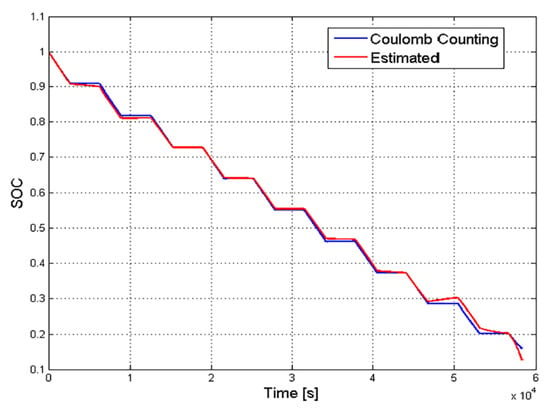
To estimate the SoC, the discharge current and voltage data of the experimental procedure described above were used. To avoid the temperature of the cell increasing due to the current, the cell discharged with current pulses at a rate of 0.13 C. The temperature of the cell is kept constant at 25 °C and the initial SoC was 100%. Figure 9 shows the results obtained in the estimation of the SoC. The RMSRE obtained was 1.19%, which is similar or less than those found in the literature [4,5,6,7,8,9,10,11,12,13,21]. This error is acceptable and it was observed that the prediction of the SoC using EKF, in each instant managed to follow the reference SoC. In each iteration the EKF obtained the output voltage of the model based on the measured current and the state variables. This allowed us to compare the response of the model to the dynamics of voltage measured experimentally.

Figure 10 shows the comparison of the output voltage estimated by the algorithm and the experimental voltage. The voltage behavior was due to the discharge current profile, where the current was greater than zero for 45 min and was zero for 75 min. When the current was zero the cell voltage increased until the open circuit voltage was reached, as seen in more detail near the cutoff voltage. Then when the current was greater than zero the cell voltage decreased [14].

In Figure 10, it can be seen that the estimated voltage followed the dynamics of the voltage measured in the laboratory. This is due to the fact that an accurate model was used to represent the relationship between V_OCV and SoC.

6. Conclusions

In this research, a method was developed to identify an equivalent electrical circuit of a Li-ion cell. The results obtained showed that the behavior of the cell depends on its SoC and temperature. From the impedance spectrum, a model of a Li-ion cell was derived, where it was verified that the cell had fractional properties. The adjustment by the genetic algorithm allowed the accurate identification of an electrical model of the cell. The uncertainty of the adjustment was 4%, therefore the adjustment provided good accuracy to predict the dynamic effects of the battery. With regard to modeling the parameters based on the SoC and the temperature, the models with neural networks provided better results with a RMSRE of 5% for both the Rs and W. The RMSRE for the parameters R₁ and C₁ were to be 13% and 10%, respectively. Therefore, the characterization of the cell was carried out under different conditions allowing us to understand the behavior of a Li-ion cylindrical cell more precisely. This is important for monitoring the charge/discharge process in order to know the state of charge or state of health of the battery precisely.

While the parameterization of the model was carried out for different SoC and temperature conditions, in the SoC estimation, each parameter of the model was considered as constant and calculated as the average of the measured values at different SoCs and a fixed temperature of 25 °C. For the SoC estimation, the extended Kalman filter based on a Randles model was used. The maximum error of estimation of the SoC was 1.19%.

This algorithm can be very useful since the battery is a critical component, which makes the precision of measuring the SoC more and more important. Future research can improve the estimation by considering the variation of the SoC and temperature.

References

1. Baba, N.; Yoshida, H.; Nagaoka, M.; Okuda, C.; Kawauchi, S. Numerical simulation of thermal behavior of lithium-ion secondary batteries using the enhanced single particle model. J. Power Sources 2014, 252, 214–228. [Google Scholar] [CrossRef]
2. Al Nazer, R.; Cattin, V.; Grajon, P.; Montaru, M. A new optimization algorithm for a Li-ion battery equivalent electrical circuit identification. In Proceedings of the 9th International Conference of Modeling, Optimization and Simulation, Bordeaux, France, 6–8 June 2012. [Google Scholar]
3. Vyroubal, P.; Kazda, T. Equivalent circuit model parameters extraction for lithium ion batteries using electrochemical impedance spectroscopy. J. Energy Storage 2018, 15, 23–31. [Google Scholar] [CrossRef]
4. Mastali, M.; Vazquez, J.; Fraser, R.; Fowler, M.; Afshar, S.; Stevens, M. Battery state of charge estimation using Kalman filtering. J. Power Source 2013, 239, 294–307. [Google Scholar] [CrossRef]
5. Sepasi, S.; Ghorbani, B.; Liaw, Y. A novel on-board state of charge estimation method for aged Li-ion batteries based on model adaptive extended Kalman Filter. J. Power Sources 2014, 245, 337–344. [Google Scholar] [CrossRef]
6. Hu, X.; Li, S.; Peng, H.; Sun, F. Robustness analysis of state of charge estimation methods for two types of Li-ion batteries. J. Power Sources 2012, 217, 209–219. [Google Scholar] [CrossRef]
7. Xiong, R.; Sun, F.; Chen, Z.; He, H. A data-driven multi-scale Extenden Kalman Filtering based parameter and state estimation approach of lithium-ion polymer battery in electric vehicles. Appl. Energy 2014, 113, 463–476. [Google Scholar] [CrossRef]
8. Xiong, R.; Sun, F.; Gong, Z.; Gao, C. A data-driven based adaptive state of charge estimator of lithium-ion polymer battery in electric vehicles. Appl. Energy 2014, 113, 1421–1433. [Google Scholar] [CrossRef]
9. He, W.; Williard, N.; Chen, C.; Pecht, M. State of charge estimation for electric vehicle batteries using unscented Kalman filter. Microelectron. Reliab. 2013, 1, 840–847. [Google Scholar] [CrossRef]
10. Sun, F.; Hu, X.; Zou, Y.; Li, S. Adaptive unscented Kalman filtering for state of charge estimation of a lithium-ion battery for electric vehicles. Energy 2011, 36, 3531–3540. [Google Scholar] [CrossRef]
11. Andre, D.; Apple, C.; Soczka-Guth, T.; Uwe, D. Advanced mathematical methods of SOC and SOH estimation for lithium-ion batteries. J. Power Sources 2013, 224, 20–27. [Google Scholar] [CrossRef]
12. Sun, F.; Xiong, R.; He, H. Estimation of state of charge and state of power capability of lithium-ion battery considering varying health conditions. J. Power Sources 2014, 259, 166–176. [Google Scholar] [CrossRef]
13. Li, J.; Klee, C.; Guenther, C.; Danzer, M. A comparative study of state of charge estimation algorithms for LiFePO4 batteries used in electric vehicles. J. Power Sources 2013, 239, 244–250. [Google Scholar] [CrossRef]
14. Burgos, C.; Orchard, M.; Kazerani, M.; Cardenas, R.; Sáez, D. Particle-Filtering estimation of maximum available power state in Lithium-Ion batteries. Appl. Energy 2016, 161, 349–363. [Google Scholar] [CrossRef]
15. Xia, B.; Sun, Z.; Zhang, R.; Cui, D.; Lao, Z.; Wang, W.; Sun, W.; Lai, Y.; Wang, M. A Comparative Study of Thre Improved Algorithms Based on Particle Filter Algorithm in SOC Estimation of Lithium Ion Batteries. Energies 2017, 10, 1149. [Google Scholar] [CrossRef]
16. Xia, B.; Sun, Z.; Zhang, R.; Cui, D.; Lao, Z. A Cubature Particle Filter Algorithm to Estimate the State of the Charge of Lithium-Ion Batteries Based on a Second-Order Equivalent Electric Circuit. Energies 2017, 10, 457. [Google Scholar] [CrossRef]
17. Zheng, L.; Zhu, J.; Wang, G.; Lu, D.; He, T. Differential voltage analysis based state of charge estimation methods for lithium-ion batteries using extended Kalman Filter and Particle Filter. Energy 2018, 158, 1028–1037. [Google Scholar] [CrossRef]
18. Ye, M.; Guo, H.; Xiong, R.; Yu, Q. A double-scale and adaptive particle filter-based online parameter and state of charge estimation method for lithium-ion batteries. Energy 2018, 144, 789–799. [Google Scholar] [CrossRef]
19. Xia, B.; Guo, S.; Wang, W.; Lai, Y.; Wang, H.; Wang, M.; Zheng, W. A State of Charge Method Based on Adaptive Extended Kalman Filter-Particle Filtering for Lithium-Ion Batteries. Energies 2018, 11, 2755. [Google Scholar] [CrossRef]
20. Baudry, P.; Neri, M.; Gueguen, M.; Lonchampt, G. Electro-thermal modelling of polymer lithium batteries for starting period and pulse power. J. Power Sources 1995, 54, 393–396. [Google Scholar] [CrossRef]
21. Xu, J.; Chir, C.; Cao, B.; Cao, J. A new method to estimate the state of charge of lithium-ion batteries based on the battery impedance model. J. Power Sources 2013, 233, 277–284. [Google Scholar] [CrossRef]
22. Monje, C.; Chen, Y.; Vinagre, B.; Xue, D.; Feliu, V. Fractional-Order System and Controls; Springer: Berlin, Germany, 2010; pp. 4–8. [Google Scholar]
23. Safa, M.; Hao, Y.; Chamaani, A.; Adelowo, E.; Chawla, N.; Wang, C.; El-Zahab, B. Capacity Fading Mechanism in Lithium Sulfur Battery Using Poly (ionic liquid) Gel Electrolyte. Electrochim. Acta 2017, 258, 1284–1292. [Google Scholar] [CrossRef]
24. Chamaani, A.; Safa, M.; Chawla, N.; El-Zahab, B. Composite Gel Polymer Electrolyte for Improved Cyclability in Lithium-Oxygen Batteries. ACS Appl. Mater. Interfaces 2017, 9, 33819–33826. [Google Scholar] [CrossRef] [PubMed]
25. Wang, B.; Eben Li, S.; Peng, H.; Liu, Z. Fractional-order modeling and parameter identification for lithium-ion batteries. J. Power Sources 2015, 293, 151–161. [Google Scholar] [CrossRef] [Green Version]
26. Wijewardana, S.; Vepa, R.; Shaheed, M. Dynamic battery cell model and state of charge estimation. J. Power Sources 2016, 308, 109–120. [Google Scholar] [CrossRef]
27. Zhang, W.; Yen, G.; He, Z. Constrained Optimization via Artificial Immune System. IEEE Trans. Cybern. 2014, 44, 185–188. [Google Scholar] [CrossRef] [PubMed]
28. Precup, R.; Sabau, M.; Petriu, E. Nature-inspired optimal tuning of input membership functions of Takagi-Sugeno-Kang fuzzy models for Anti-lock Braking Systems. Appl. Soft Comput. 2015, 27, 575–589. [Google Scholar] [CrossRef]
29. Elsayed, S.; Sarker, R.; Ray, T.; Coello, C. Consolidated optimization algorithm resource-constrained project scheduling problems. Inf. Sci. 2017, 418, 346–362. [Google Scholar] [CrossRef]
30. The MathWorks. Genetic Algorithm and Direct Search Toolbox for Use with MatLab, version 1; The MathWorks: Natick, MA, USA, 2004. [Google Scholar]
31. Perez, H.; Siegel, J.; Lin, X.; Stephanopoulos, A.; Ding, Y.; Castanier, M. Parameterization and validation of an integrated electro-thermal cylindrical LFP battery model. In Proceedings of the ASME 5th Annual Dynamic Systems and Control Conference, Fort Lauderdale, FL, USA, 17–19 October 2012. [Google Scholar]
32. Isasi, P.; Galván, I. Redes de Neuronas Artificiales: Un Enfoque Práctico; Pearson Education S.A.: Madrid, Spain, 2004; pp. 1–22. [Google Scholar]
33. Grewal, M.; Andrews, A. Kalman Filtering: Theory and Practice Using MatLab; John Wiley & Sons, Inc.: Hoboken, NJ, USA, 2015; pp. 169–224. [Google Scholar]
Figure 1. The EEC model of the Li-ion cell.
Energies 12 00681 g001
Figure 2. Nyquist diagram of an experimentally obtained Li-ion cell.
Energies 12 00681 g002
Figure 3. Nyquist diagram of an experimentally obtained Li-ion cell.
Energies 12 00681 g003
Figure 4. Comparison of the experimental and estimated impedance spectrum at SoC = 40% and 25 °C.
Energies 12 00681 g004
Figure 5. The EEC parameters for different temperatures.
Energies 12 00681 g005
Figure 6. Artificial Neural Network with two inputs, two layers and one output.
Energies 12 00681 g006
Figure 7. Estimated Rs with: (a) Parametric identification of the electric model of the cell; (b) the empirical equation; and (c) the ANN, for different SoC and temperatures.
Energies 12 00681 g007
Figure 8. Kalman filter algorithm equations.
Energies 12 00681 g008
Figure 9. Result of the SoC estimation with EKF.
Energies 12 00681 g009
Figure 10. Comparison of the experimental and estimated voltage of the cell.
Energies 12 00681 g010