The Analysis of Leading Edge Deformations on Turbomachine Blades


1
School of Energy and Power Engineering, Beihang University, Beijing 100191, China
2
National Key Laboratory of Science and Technology on Aero-Engine Aero-Thermodynamics, Beihang University, Beijing 100191, China
*
Author to whom correspondence should be addressed.
Energies 2019, 12(4), 736; https://doi.org/10.3390/en12040736
Submission received: 29 January 2019
/
Revised: 17 February 2019
/
Accepted: 19 February 2019
/
Published: 22 February 2019
Abstract
:With recent advancements in the development of material and manufacturing technology, the leading edge geometry of turbomachine blades has attracted widespread attention. “Sharp” leading edges always have a better aerodynamic performance, though it is prone to deformations easily. Thus, flat plates and real compressor cascades with different leading edge deformations were investigated to study the influence, which is applicable for thin blades at low speeds. Different boundary layer characteristics, including the velocity profile, transition process, and loss, are compared. The results show that there are several kinds of contradictory influence mechanisms and that the final phenomenon is closely related to the condition of the original boundary layer. In low turbulence, with large and laminar separation, the deformations can suppress separation and decrease loss. In high turbulence, with short and transitional separation, deformations can promote the transition process and increase the loss. The sensitivities of different the original leading edge shapes are also compared. This indicates that a good design always has a better robustness at low turbulence values, while it is worse at high turbulence values. The cascade experiment and simulation show that the deformation influence is similar to flat plates and that it is enlarged near the hub, which affects the corner separation.
1. Introduction
For the sake of energy conservation and cost saving, the turbomachine blades should be improved in two aspects, namely, increasing the mechanical efficiency and prolonging the service life. Optimizing the geometry of the front of blades (leading edge), which could be implemented by simply replacing or re-profiling the blades without an expensive redesign can achieve these two challenges. Norris [1] found in his case study of the Rolls Royce Trent 700EP that the profile loss was reduced by 30% and that the fuel was reduced by 1.3% with the blades’ circular leading edge updated by the ellipse.
For the aero-engine or other turbomachines, the blade profile loss is mainly caused by the suction surface boundary layer, except for a large negative incidence. The development process of the boundary layer is quite complex. Separation, transition, reattachment, and relaminarization can all appear. At the leading edge region, the velocity of the boundary layer outer edge increases and then decreases because of the wall curvature [2]. This makes it very easy to cause separation and transition, which brings more loss [3]. The present study has involved several aspects, such as the leading edge shape, incidence, Reynolds number, free-stream turbulence, and Mach number.
The “Sharp” leading edge shapes or continuous curvature designs are found to be capable of reducing the pressure variation and suppress separation. In Carter [4] research on a series of circular leading edges, the one having the smallest radius got the widest operating range. Walraevens and Cumpsty [5] tested both circular and 1.89:1 elliptical leading edges on a flat plate at a subsonic level. It was found out that the flow around the circular leading edge separated while the elliptical leading edge remained attached. Wheeler et al. [6,7] investigated the behaviour of a circular leading edge and 3:1 elliptical leading edge on a stator in a low-speed compressor. For the circular leading edge, separation and transition happened while the flow around the elliptical leading edge remained attached and laminar, which reduced the profile loss by 32%. At the leading edge, a large change in the surface curvature causes a small “spike” in the surface pressure distribution. Goodhand and Miller [8] investigated the spike effect and presented a spikeless design (with continuous curvature), which allowed a leading edge thickness of 4% and 3%, greater than the elliptical and circular leading edges for avoiding separation, respectively.
For most turbine compressors, the Reynolds numbers based on chord Rec are typically between 0.6 × 10⁶ and 4 × 10⁶ [9] (the Reynolds numbers based on the leading edge half thickness Ret are typically between 0.3 × 10⁴ and 0.9 × 10⁴ for aero-engine). The free-stream turbulence intensities (Tu) are around 4% [10] (around 12% when the wake comes). Steinert and Starken [11] conducted a cascade experiment at Ret = 4.1 × 10⁴ and Tu = 2.5%, and showed that the boundary layer stayed laminar over a wide range of incidences. The Ret of this experiment is much higher than the practice. Therefore, at the leading edge region, the transition will not occur unless there is a separation or wake. In other words, the transition in a separation bubble is the most common structure of the leading edge boundary layer. Walraevens and Cumpsty’s [5] experiment showed that the positive incidence and free-stream turbulence intensity both have a remarkable effect on the transition process, which forms a shorter separation bubble. However, the Reynolds number only exerts a weak effect on the boundary layer.
For most turbomachine blades, they always work in severe conditions. There are many unfavourable factors which restrict the blades’ performance, such as external loading [12] or susceptibility to damage [13]. Therefore, the blades’ performance significantly impacts the aerodynamic efficiency and mechanical performance. The current research on the blades’ leading edge also develops towards the engineering practice. Apart from the aerodynamic efficiency of the design conditions, another factor that determines the performance of the leading edge is the operating life, which is influenced by two major aspects, namely, the capacity to resist deformations (basically depend on the material) and the aerodynamic reaction to non-designed deformations.
Non-designed deformations such as fabrication tolerances, blade degradations and maintenance, repair and overhaul (MRO) processes of the blade’s leading edge geometry always leads to a loss increase, and thus attracts researchers’ attention. Blunt is the most common type [14], which makes the efficiency drop significantly [14,15]. The sensitivity of the leading edge is also studied, proving that small geometrical changes have a linear or second order influence [16,17].
There are two questions which should be further studied. First, for turbomachine blades, how does the boundary layer character such as velocity profile, transition process or loss change in a damaged leading edge? Second, are different leading edge designs endowed with different sensitivities? The final goal is to find out the leading edge design with the best aerodynamic performance and the highest robustness. Based on these two questions, the research was divided into two parts. In the first part, a flat plate with single elliptical leading edge shape was investigated to find out how the boundary layer changes at different turbulence and deformation levels. In the second part, another two leading edge shapes were added to investigate their sensitivity.
The flat plate research ignores the two conditions of real blades, namely, adverse pressure gradient and three-dimensional flow. Adverse pressure gradient makes the boundary layer worse after the leading edge region, which may lead to the separation and transition at the middle area or the trailing edge. Thus, it raises the question of how the boundary layer downstream development is influenced by its early change. The three-dimensional flow includes vortices, corner separation and other structures [18,19,20,21,22,23,24,25,26]. Especially for corner separation, it always limits the blade loading and incidence range because of serious impacts [22,23,24,25,26]. In Gbadebo’s study [21], we showed that the leading edge roughness could affect the corner separation. This confirmed the influence of the early boundary layer in the 3D flow field. Goodhand and Miller [27] compared circular and elliptical leading edges of a low-speed compressor stator and showed that the circular leading edge increased the total loss by 72%. A similar phenomenon was observed by Lyu Jianbo [28] who compared both shapes on a highly-loaded compressor cascade. Based on these research articles, a cascade with different original leading edge shapes and deformations was investigated to cover the shortage of flat plate research.
2. Computation Methods
The research is based on the experiment conducted by Walraevens and Cumpsty [5]. The flat plate is aerodynamically analyzed by means of the steady 2D-RANS simulation of the commercial software, CFX-12.0. It uses the Shear-Stress-Transport (SST) turbulence model [29,30,31] and gamma-theta transition model [32,33]. The mesh type is H-O-H with local refinement, as shown in Figure 1a. The size of the wall first mesh is controlled to ensure y+ < 1. Convergence of the mesh is investigated by varying the mesh resolution. The number of nodes varies from around 71,000 to 337,000. Figure 1b shows the wall static pressure confidence Cp distribution of the elliptical leading edge at Tu = 7%. It has a good convergence when the mesh number is more than 137,000. In order to ensure accurate data processing and make the mesh expansion ratio less than 1.1, the final total number of nodes amounts to around 226,000.
The research requires detailed parameters of the boundary layer so that the verification of the simulation includes three aspects, that is, the wall pressure confident Cp distribution, defined in Equation (1), shown in Figure 2a,b; the boundary layer momentum thickness θ, defined in Equation (2), shown in Figure 2c; and shape factor H among the aerofoil, defined in Equation (3), shown in Figure 2d. The horizontal axis has a relative arc length S, defined in Equation (4). This study also tests the scope of the application of the geometry, incidence and turbulence intensity. Circ.LE is the circular leading edge (with a ratio of 1). Ellip.LE is the elliptical leading edge with a ratio of 1.89. The results show that the agreement can be ensured at turbulence ranges from 0% to 7% and incidence ranges from 0 deg to 2 deg. The pressure plateau caused by laminar separation and stopped by transition [34] can be exactly simulated in the leading edge region. Actually, the experiment contained other incidence and turbulence conditions, while the computation could not have the equivalent accuracy. Therefore, the study was performed at a leading edge thickness Reynolds number of 3000 and free-stream turbulence intensity values from 0 to 7%.
where p is the wall static pressure, ptin is the inlet total pressure, u is the local velocity, U is the inviscid velocity, δ is the boundary layer thickness (u = 0.99 U), Sl is the distance around the surface from the nose of the leading edge, and t is the thickness of the leading edge (for the present, tests the thickness of the flat plate, as Figure 3 shows).
Cp = (p − ptin) / ptin
S = 2Sl / t
The basic leading edge shape is an ellipse with a ratio of 1.89 [2] (named ORI, which is also applied in Section 3.3). In order to analyze the influence of the leading edge deformations, blunt and wedge deformations are manufactured, as shown in Figure 3. BLUNT is a cut vertical to the axis of symmetry at the nose of the leading edge. WEDGE is a cut between the nose and a certain point at the leading edge surface. The deformations level ε, defined in Equation (5), is 2%, 6% or 10%. These two kinds of deformations were used to simulate the damage caused by external factors in manufacturing and working.
where εd is the horizontal position of the cut and lLE is the length of the leading edge.
ε = εd / lLE
3. Results and Analysis
3.1. Deformations Influence of Elliptical Leading Edge
Figure 4 shows the distribution of Cp in the front of the surfaces of ORI; 10% BLUNT, the BLUNT at ε = 10% and 10% WEDGE, respectively, at Tu = 5%. The relative arc length S is used for the X-axis, which demonstrates the relationship between pressure and the distance of development in the early stage. The Cp distribution of the ORI is relatively smooth. By contrast, the 10% BLUNT and 10% WEDGE appear as spikes because of the metal angles. After the spikes, the Cp of different leading edges were almost the same, indicating that the deformations at ε < 10% can only affect the early flow environment. It can be seen that the curve of the 10% BLUNT is nearly horizontal at the beginning and nearly vertical before the spike, showing that the BLUNT can represent the worst condition at certain ε values and the WEDGE can represent an intermediate level.
Shape factor H (defined in Equation (3)) and the normal average turbulence intermittency γ’ reflect the development process of the suction surface boundary layer in a more detailed manner. The definition of γ’ is
where γ is the turbulent intermittency.
H can reflect the velocity profile in the boundary layer. The increase of H indicates that the velocity profile has deteriorated due to the wall curvature or adverse pressure gradient. The laminar boundary layer separates when H reaches 2.5 to 3 and reattaches when H comes back to around 3. The turbulent boundary layer stays when H is around 2. The maximum of H in the boundary layer separation region Hmax indicates the strength of the separation bubble. γ’ can reflect the process of boundary layer transition. It is less than 0.2 for the laminar boundary layer. The transition appears when the value of γ’ begins to increase and competes when the value of γ’ approximates to about 0.9.
At Tu = 0, The ORI boundary layer can be regarded as the reference, as shown in Figure 5. A few spikes of H and θ formed before S = 20.78 (the reattachment point) because there are some strong laminar separation bubbles. In the separation region, the Hmax amounts to 7.17, θ reaches 0.516 mm, and γ’ achieves 0.087. After reattachment, γ’ stays at a low level, showing that the boundary layer stays in the laminar region. It can be seen from Figure 5 and Figure 6 that different boundary layers all have steady states after the point of about S = 20. Therefore, this point can be taken as the investigation point S0 (it also applies to the following research). For ORI, at S0, θ starts to rise from 0.452 mm in a nearly linear way. γ’ achieves 0.041 and it grows slightly.
The BLUNT series promotes the transition process and suppresses separation. For 2% BLUNT, the reattachment point is put forward to S = 12.3. At S0, θ reaches 0.455 mm and γ’ achieves 0.106 (+0.065). Unexpectedly, the WEDGE series leads to stronger separation, as shown in Figure 6. For 2% WEDGE, the reattachment point is at S = 13.99, at S0, θ achieves 0.559 mm (+0.107 mm), which is obviously higher than the others. It should be noted that for all leading edges, after reattachment, θ with a higher γ’ increases faster (this rule applies to other computation conditions).
Figure 7 shows the influence of BLUNT at Tu = 5% (Tu = 3% is similar). For ORI, a relatively weak leading edge separation bubble forms. The reattachment point is at S = 7.58. In the separation region, the Hmax amounts to 5.56 and γ’ achieves 0.43. After reattachment, γ’ drops to 0.12 (relaminarization). However, it grows again. At S0, θ reaches 0.445 mm and γ’ achieves 0.232.
Deformations bring two negative influences: intensifying the strength of the leading edge separation bubble and the promoting transition process. However, the impact degree of either the BLUNT or WEDGE is small unless the transition is completed in a separation bubble. For 6% BLUNT, the Hmax amounts to 5.59. At S0, θ reaches 0.455 mm (+0.01 mm) and γ’ achieves 0.25. This phenomenon is similar for the WEDGE. However, it is weaker than the BLUNT’s phenomenon. For 6% WEDGE, as shown in Figure 8, the Hmax amounts to 5.57. At S0, θ reaches 0.45 mm and γ’ achieves 0.243. It should be noted that 10% BLUNT can be much more influential. The Hmax reaches 5.7 (+0.14) and the separation directly leads to the transition completion, which leads to a dramatical loss increase. At S0, γ’ stays at 0.87 (the total turbulence boundary layer) and θ reaches 0.56 mm (+0.105 mm) with much more growth than others.
When the inlet turbulence achieves 7%, as shown in Figure 9 and Figure 10, the boundary layer separation can directly lead to the complete transition. For ORI, the Hmax amounts to 4.78. The reattachment point is at S = 5.7. At S0, θ reaches 0.534 mm and γ’ stays at around 0.87. The main influence of the deformations is putting the transition forward and, thus, increasing the loss. For 10% BLUNT, as shown in Figure 9, the point where γ’ achieves 0.6 is put forward from S = 7.32 to S = 5.96. At S0, θ reaches 0.586 mm (+0.052 mm). Similarly, for 10% WEDGE, as shown in Figure 10, at S0, θ reaches 0.55 mm (+0.016 mm).
Loss penalty ∆θ is the loss caused by deformations; the definition is
∆θ = θDEFORMATION − θORI
It should be noted that after S0, there is no difference among γ’ in all the series, but deformations also accelerate the increase of θ. This means that ∆θ keeps growing as the boundary layer develops downstream. For instance, the γ’ of ORI and 10% BLUNT both stay at 0.87 after S0, while at S0, ∆θ is 0.052 mm and at S = 40, ∆θ increases to 0.063 mm.
Through the above analyses of the boundary layer parameters at turbulence ranges from 0 to 7%, the influence mechanisms of leading edge deformations can be summarized. This should be divided into three parts. First, at low free-stream turbulence, the boundary layer keeps laminar and has a large leading edge separation bubble, as shown in Figure 11a. In this condition, relatively serious deformations (such as BLUNT) will make the separation bubble weaker and θ drops due to the large pressure disturbance. On the contrary, small deformations (such as WEDGE) will make the separation bubble stronger and θ increases. Second, at the middle level of free-stream turbulence, the boundary layer transition process is slow and the separation bubble is medium, as shown in Figure 11b. Deformations make a small influence at low ε levels. With the expansion of ε, deformations can promote the transition process obviously and bring about higher loss. Third, when the inlet turbulence level is up to 7%, the leading edge separation bubble is very weak because the transition completes just after the separation begins, as shown in Figure 11c. The main influence of the deformations is in promoting the transition process. In this condition, the loss penalty ∆θ has a positive correlation with ε.
It should be noted that instead of free-stream turbulence, the separation bubble and transition process both decide the influence mechanism. These two questions have captured researchers’ attention for decades [34,35,36,37,38]. Hatman and Wang [35] distinguished the separation bubble as three modes, shown in Figure 12. The scale of the separation bubble and transition speed has a negative correlation. It is very meaningful that there is a one-to-one correspondence between Figure 11 and Figure 12. In other words, different influence mechanisms are only suited to different separation modes.
The influence of leading edge deformations can be extended to a bigger incidence range. Walraevens and Cumpsty’s study [5] showed that increasing incidence can generate transition and suppress the separation bubble, which makes the boundary layer similar to a higher turbulence. Therefore, it can be speculated that the influence of the leading edge deformations increases with the incidence.
Figure 13 shows the result of ORI and 6% BLUNT at i = 2 deg. For ORI, at Tu = 0, the leading edge separation is extra strong. The Hmax amounts to 11.2 and the reattachment point is at S = 10.14. At S0, θ reaches 1.43 mm. For 6% BLUNT, the Hmax amounts to 10.41 and θ reaches 1.52 mm (+0.09 mm) at S0. With the turbulent inlet, the Hmax and θ decrease obviously, indicating that a short transitional separation bubble occurs, which is similar to the condition at i = 0 deg and Tu = 7%. As expected, the deformation influence is also similar to that condition. Taking the result at Tu = 3% as an example, for ORI, the Hmax amounts to 7.88, and the reattachment point is at S = 5.47. At S0, θ reaches 1.427 mm. For the 6% BLUNT, the Hmax amounts to 7.46 and the reattachment point is at S = 5.51. At S0, θ reaches 1.525 mm (+0.1 mm).
3.2. Different Leading Edge Sensitivities
In order to investigate the sensitivity of different leading edge shapes, apart from the involved elliptical leading edge, named E1.89 in this subsection, another two series are added to the research, as shown in Figure 14. One is an elliptical leading edge with a ratio of 1.2, named E1.2. The other one is a continuous curvature leading edge with a ratio of 1.89, named CL. The continuous curvature design uses the three-order Bézier curve [39]. The design principle is to ensure that the wall curvature is continuous at the tangent point and to keep the shape as similar to E1.89 as possible. The results show that the continuous curvature design could not perform better than E1.89, which is opposite to the previous research articles [8] (a real blade always has a positive wedge angle and larger leading edge length). However, it is still significant to compare and help summarize the sensitivity rules of different leading edge shapes.
The research compares the θ of different leading edges at the point of S = 50 (approximating to the chord length). Based on the above analysis, the influence mechanisms of the leading edge deformations are different in low free-stream turbulence, middle free-stream turbulence, and high free-stream turbulence, respectively. Therefore, the three states should be distinguished.
The low turbulence condition is shown in Figure 15. It should be especially explained that in the following figures, there are two vertical axes both in the left and right because the θ of E1.2 is much higher than others and, thus, it is based on the right-side vertical axis. At the same time, the increments of the two axes are the same in order to reflect the deformation influence. For the E1.89 series, the BLUNT makes the profile loss increase and then decline. The greatest change occurs at ε = 2% and θ grows by 10.19% (+0.063 mm). The smallest influence occurs at ε = 10% and θ decreases by 1.7% (–0.011 mm).
The E1.2 series has a high θ level as a result of more serious separation. At ε = 2%, θ increases by 2.59% (+0.032 mm) and at ε = 10%, θ decreases by 2.79% (–0.035 mm). The WEDGE’s influence is larger than the BLUNT’s influence. At ε = 2%, the loss of E1.89 increases by 10% (+0.061 mm), and the loss of E 1.2 increases by 11.48% (+0.142 mm). For the CL series, the deformations influence is much more obvious. The greatest decline amounts to 37.25% (–0.372 mm) at 6% BLUNT. This is because the CL leading edge causes a larger separation bubble than E1.89 and the deformations ability of the suppressing separation is strengthened.
The trend of E1.89 and E1.2 is similar. When ε is small, profile loss increases. However, with the expansion of ε, the loss can decrease because of suppressed separation bubble. This conflict effect indicates a maximum loss penalty ∆θmax. The result shows that ∆θmax of E1.89 is larger than 19.58% (+0.121 mm), and larger than 15.6% (+0.193 mm) of E1.2 series.
Figure 16 shows the condition of middle free-stream turbulence. E1.2 only has this condition at Tu = 3%. At Tu = 5%, a short transitional separation bubble is formed, and the condition should be classified to high turbulence. Similarly, CL does not have this condition at all. The state at Tu = 3% is taken as an example. For E1.89, 2% BLUNT reduces θ by 0.78% (–0.05 mm), and 6% BLUNT rises θ by 1.67% (+0.011 mm). Indeed, 10% BLUNT leads to transition near the leading edge and raises θ by 68.6% (+0.45 mm). For E1.2, the trend is similar and gentler. ∆θ ranges from –0.7% to 0.17%. The influence of WEDGE is similar to BLUNT’s, but the impact degree is much lower.
Middle free-stream turbulence is the most common working condition of turbomachine blades at present. The separation bubble is reduced to a great extent and the transition process is mainly related to free-stream turbulence. This makes the deformations influence insignificant. If the deformations are large enough to affect the transition process, the loss changes obviously. The results of the E1.89 approximate to a second-order function and the results of E1.2 approximate to a linear function. This indicates that E1.89 is more sensitive to deformation even though the θ of E1.89 is still lower than E1.2 at ε = 10%. Besides, it should be noted that for E1.89, the θ at Tu = 5% is almost the upper shift of Tu = 3%, regardless of BLUNT or WEDGE. The separation bubble at Tu = 5% is very similar to that at Tu = 3%, with an incomplete transition and relaminarization. Therefore, a reasonable hypothesis is proposed. The influence of the leading edge deformations cannot be changed by turbulence at a certain mode of the separation bubble.
Figure 17 shows the condition of high turbulence. This condition applies to E1.89 at Tu = 7%, E1.2 at Tu = 5%, 7%, and CL at Tu = 3%, 5%, 7%. In this condition, the size of the leading edge separation bubble is very small and the transition is completed just after the separation begins. The profile loss has a close positive relationship with ε. At Tu = 7%, for BLUNT, the θ of E1.89 ranges from –0.26% to 5.24% (+0.057 mm), and the θ of E1.2 ranges from 0.09% to 0.8% (+0.01 mm). Their trends both approximate to a second-order function. The θ of CL ranges from –0.27% to 1.8% (+0.021 mm) in its own trend. Similar to the middle free-stream turbulence condition, WEDGE is consistent with BLUNT, while the impact degree is smaller.
For both the E1.2 series and CL series, the results at different turbulence values are almost parallel, which are similar to the E1.89 series at middle turbulence. This supports the hypothesis that the influence of the leading edge deformations remain the same when the basic boundary layer separation mode is maintained unchanged. This phenomenon can also be applied to the Reynolds number, as Section 3.3 discusses. Therefore, when the leading edge sensitivity is investigated, rather than other working conditions, only the separation mode is required.
By comparing the sensitivity of different leading edge shapes, it can be concluded that the sensitivity is closely related to the original boundary layer development in the early state. For instance, at low free-stream turbulence, the separation bubble brings a large loss and it is very sensitive to the disturbance brought by deformations. At this time, the excellent leading edge design is endowed with not only good aerodynamic performance, but also an optimized sensitivity. When the free-stream turbulence increases, the loss caused by the turbulent boundary layer gradually occupies a larger percentage. The excellent design can usually effectively restrain the transition process, but the weakness is that it easily becomes very unsteady, making it very sensitive to deformations. Thus, for the leading edge optimization, it is important to consider the influence of deformations on the blade performance. Even if the problem is ignored, the leading edge optimizing still has a practical meaning. As shown in Figure 15 to Figure 17, the aerodynamic performance of E1.89 is better than E1.2 in all cases, even though a 63.4% loss penalty occurs.
3.3. Compressor Cascade Investigation
In practice, there are two questions that flat plate research has neglected that should be further discussed. One is the influence of deformations on the velocity profile in the downstream boundary layer. The other is the influence under 3D condition (the region near the hub). Therefore, an investigation on real compressor cascades is conducted.
In the flat plate, after the leading edge separation, the boundary layer develops with zero pressure gradient and zero wall curvature. Thus, the shape factor H remains stable. However, in the real cascade, the boundary layer inevitably faces a negative pressure gradient and convex wall curvature. Once the early velocity profile has changed, it is difficult to recover and the whole boundary layer is affected. The loss cannot be ignored, especially in the high-lift blade design [40,41], where the mid-blade separation must be paid attention to.
Table 1 depicts the cascade physical parameters. The blade is designed by the National Key Laboratory of Science and Technology on Aero-Engine Aero-Thermodynamics, Beihang University. The leading edge includes two original shapes. One is an ellipse with a ratio of 1.89; the other is an integrated design with a continuous curvature, as shown in Figure 18. Owing to the larger wedge angle and leading edge length, the integrated design performs better than an ellipse for the disappearance of the leading edge separation. The deformations include the BLUNT and WEDGE of ε = 2%, as Table 2 describes. It ensures there is no influence on blade load.
The experiment is carried out in a low-speed tunnel of the laboratory. The conditions are as follows. The environment pressure Pout = 101,000 Pa, the Temperature T = 15 °C, the inlet free-stream turbulence Tu = 2.5%. the inlet relative total pressure Ptin = 80.5 Pa and 160.5 Pa, which makes the Reynolds number based on the leading edge thickness Ret = 2500 and 3500. At Ptin = 80.5 Pa, the middle area separation appears in the suction surface, however, at Ptin = 160.5 Pa, the middle area separation does not appear.
CFX-12.0 is used for numerical simulations. The SST turbulence model and gamma-theta transition model are used similarly for flat plate computation. The type of the mesh is also H-O-H, and there are two layers of the O-type mesh surrounding the blade with local refinement. The convergence of the mesh was investigated similar to the flat plate. The total number of nodes amounts to around five million, as shown in Figure 19. The simulation used the total pressure inlet and static pressure outlet as the boundary condition. The inlet total pressure and free-stream turbulence were the same as that of the experiments. The outlet static pressure was atmospheric pressure.
The verification of the simulation includes two aspects: the wall pressure confident distribution at the middle height of the blade (Figure 20a) and exit flow field (Figure 20b). The difference between the experiment and CFX computation was located mainly in the region near the hub since the hub boundary layer scale is larger in the experiment than the CFX computation. However, the accuracy of the suction surface boundary layer can be ensured before the hub boundary layer influence.
The influence on the boundary layer velocity profile can be studied by analyzing the flow field at a middle height (z/l = 0.5) where no 3D flow appears. Figure 21 shows the θ, H and γ’ among the suction surface at Tu = 2.5%, Ret = 2500. For ORI, the same as the flat plate, a laminar separation/short bubble occurs in the leading region. γ’ increases at the leading edge separation but then decreases after reattachment (relaminarization). While downstream, H rises again, and a middle area separation occurs. The maximum level of H in this region is named Hmax’. In the middle separation region, γ’ reaches 0.9, indicating that the transition is completed. The condition is similar at Ret = 3500, thus, it is not further discussed. However, Hmax’ under this condition does not exceed 3.
For ORI, Hmax amounts to 4.22 and Hmax’ amounts to 3.38, showing that the mid-bubble separation is much weaker than the leading edge’s. For BLUNT, Hmax amounts to 4.65 while Hmax’ amounts to 3.19, meaning that the leading edge separation is promoted (similar to a flat plate) and the middle area separation is suppressed. Remarkably, at S = 8 (after leading edge separation), ∆θ is 0.005 mm at S = 35 (after leading edge separation) and ∆θ is 0.011 mm, The result is similar to the plate form aerofoil research. Therefore, it can be asserted that the reason for the major loss penalty caused by BLUNT is the larger leading edge separation bubble. For CL-ORI, there is only a middle area separation bubble and Hmax’ amounts to 3.6. For CL-WEDGE, the H distribution changes slightly. However, the γ’ decreases significantly, which makes its loss lower than other leading edges.
Although the horseshoe vortex is directly related to the leading edge geometry, in some research, this vortex is not obvious (as in this computation) or it dissipates quickly in the compressor [42]. Besides, in Goodhand’s research [27], it is the transition process that leads to the change of corner separation. Based on this fact, the suction surface boundary layer development process at a 0.05 blade height is investigated before it is influenced by the hub boundary layer. In this section, corner separation can be regarded as trailing edge separation [22].
Figure 22 shows the distribution of H, γ’, and θ for both series. The leading edge separation bubble is slightly put forward and the middle area separation bubble is put forward normally. After this (at the point of S > 0.4), H increases sharply, indicating a large trailing edge separation (corner separation). For ORI, Hmax amounts to 4.16 and Hmax’ amounts to 3.33. For BLUNT, Hmax amounts to 4.57 and Hmax’ amounts to 3.28. For CL-ORI, Hmax’ amounts to 3.82. For CL-WEDGE, Hmax’ amounts to 3.78. It should be noted that in the 0.1 blade height region, H is more critical than θ because the trailing edge separation has a decisive role in the flow. At the point of S = 30, the H of the ellipse series is about 2.6 and the H of the continuous curvature series is about 2.3. This means at this point the velocity profile of continuous curvature series is better than the ellipse series.
Figure 23 shows the Cp (defined in Equation (1)) contours at the 1.1 chord length exit of the BLUNT and CL-WEDGE, as the biggest difference in the four leading edge shapes. The contour of ORI is very close to BLUNT and the contour of CL-ORI is very close to the CL-WEDGE’s. Contours reflect the scale of corner separations. It can be seen that BLUNT is larger than CL-WEDGE, which means the trailing edge separation of BLUNT is larger than CL-WEDGE’s at a 0.05 blade length. Therefore, it can be inferred that the velocity profile penalty caused by leading edge deformation is retained afterwards in the downstream in the suction surface boundary layer. Besides, it reflects that the Reynolds number has few influences.
Figure 21 to Figure 23 show that CL-WEDGE has an excellent aerodynamic performance. Similar research has been investigated by Lu Hongzhi [43,44]. She improved a circular leading edge design with a tiny flat, as shown in Figure 24. The double suction spikes on the flat edges were much weaker than the single spike that appeared on a circular leading edge. Therefore, the loss of the boundary layer was reduced.
4. Discussion and Conclusions
At present, most serving blades have circular leading edges, but the development tendency is becoming increasingly sharper. This means that deformations are more likely to happen. Consequently, there are two practical implications to investigate deformations influence. First, it can evaluate the loss penalty of serviced turbomachine blades. Second, it can provide a reference for leading edge optimization.
Leading edge deformations affect the boundary layer in three aspects. First, the adverse static pressure at the beginning has a promoting effect on separation; second, pressure spikes caused by angles promote the boundary layer transition process; third, the pressure disturbance can suppress the laminar separation bubble. L. H. Smith Jr. [5] proposed a simple and useful method to estimate bluntness, but his method ignored the original boundary layer situation. This research fills in the gap in this aspect by focusing on how these contradictory effects of deformations interact with each other. The results show that the final influence has a close relationship with the mode of the boundary layer separation.
At low free-stream turbulence values, the loss of leading edge separation is significant. In this condition, small deformations (WEDGE) have a greater influence on promoting separation, thus, bringing more loss. Large deformations (BLUNT) can effectively suppress leading edge separation and, thus, reduces loss. The leading edge shape with a better aerodynamic performance has better robustness. As a result, at the point of the trailing edge, the loss penalty ∆θ of the ellipse with a ratio of 1.89 in the leading edge shape ranges from –1.7% to 19.58%, while being –2.8% to 15.6% with a ratio of 1.2.
With the increase of free-stream turbulence, the leading edge separation bubble reduces. There is an intermediate situation for the boundary layer in which the separation bubble and transition process both impact loss. In this condition, the deformations can suppress the separation bubble and promote the transition process, which decreases and then increases θ at a small level (∆θ/θ < 2%). It should be noted that the present purpose of most leading edge optimizations is to restrain separation and transition. An excellent leading edge can achieve relaminarization after the leading edge separation bubble, while deformations can have a devastating effect, putting forward transition and sharply increasing the loss. This nearly destroys the optimization effect. Hence, the critical value of ε for an optimized leading edge should be further studied. For an ellipse with a ratio of 1.89 for the leading edge shape, the critical value is between 6%–10%.
If free-stream turbulence continues to grow (considering wake or incidence), the transition completes just after separation begins. The separation bubble becomes tiny and insignificant. In this condition, the transition process has a decisive effect on loss and deformations can have a greater impact on it. Thus, loss increases significantly with the expansion of deformation. At ε = 10%, the θ of the ellipse with a ratio of 1.89 of the leading edge grows by 5.24% near the position of the trailing edge, while the θ of the ellipse with a ratio of 1.2 of the leading edge grows by 0.8% and the θ of the continuous curvature design grows by 1.87%. High free-stream turbulence has the most practical meaning. When the incidence is enlarged or the turbulence is increased (wake sweeping), the transition is extremely inclined to occur near the leading edge. At this time, the deformations influence is significantly larger than that predicted by the method proposed by L. H. Smith. The smaller the original boundary layer loss, the larger the loss penalty.
Deformation influence can be applied to the leading edge optimization design. There are four simple and very useful rules regarding the leading edge deformations influence. First, within a 10% deformation degree, at certain ε values, the loss of well-designed leading edge is bound to be lower. This demonstrates that in practice, leading edge optimization is meaningful even if the sensitivity question is considered. Second, when the boundary layer state is stable, ∆θ is constant at certain ε values, where the free-stream turbulence or Reynolds number has no effect. This helps to enlarge the application scope of a single research article. Third, in a real blade suction surface boundary layer, even if leading edge separation disappears through optimization, the deformations will exert influence on transition, and thus the loss. Fourth, for some high lift blades, the middle area separation usually has a larger influence than the leading edge separation. Therefore, the economic cost can be very small if the boundary layer transition is promoted and the middle area separation is restrained through design methods.
In the suction surface of real cascades, the effects of deformations can spread downstream and be amplified. The velocity profile penalty of the boundary layer near the leading edge can influence the following separation and transition. In the 2D flow field zone (far away from the hub), deformations influence is mainly on the loss. In the 3D flow field zone (near the hub), deformations also contribute to the variation of corner separation. Besides, both the experiment and computation results show that the continuous curvature leading edge with a tiny wedge deformation has an excellent aerodynamic performance. It can reduce profile loss and suppress the corner separation. For future studies, this paper provides a fruitful possibility of the leading edge optimization direction that needs further research.
Author Contributions
Conceptualization, H.L.; Data curation, L.L.; Formal analysis, L.L.; Funding acquisition, H.L.; Investigation, L.L.; Project administration, H.L.; Software, L.L.; Supervision, H.L.; Validation, L.L.; Writing—original draft, L.L.; Writing—review & editing, H.L.
Funding
This research received no external funding.
Acknowledgments
The authors would like to acknowledge the support of National Key Laboratory of Science and Technology on Aero-Engine Aero-thermodynamics, Beihang University. In this research institute, Fangfei Ning, Peng Li, and Chenyuan Liu offer help. Fangfei Ning, the professor in this research institute, provided the cascade physical parameters. The experiment work was made possible through the assistance of Peng Li. And the paper was finished with the constructive suggestions of Chenyuan Liu.
Conflicts of Interest
The authors declare no conflict of interest. The funders had no role in the design of the study; in the collection, analyses, or interpretation of data; in the writing of the manuscript, and in the decision to publish the results.
References
- Norris, G.J. Rolling enhancement: Rolls delivers upgraded Trent 700 to Airbus as threeway A330 market battle intensifies. In Aviation Week & Space Technology, 8th ed.; McGraw-Hill, Incorporated: New York, NY, USA, 2008; p. 42. [Google Scholar]
- Davis, M.R. Design of Flat Plate Leading Edges to Avoid Flow Separation. AIAA J. 1980, 18, 598–600. [Google Scholar] [CrossRef]
- Arena, A.V.; Mueller, T.J. Laminar Separation, Transition, and Turbulent Reattachment near the Leading Edge of Airfoils. AIAA J. 1980, 18, 747–753. [Google Scholar] [CrossRef]
- Carter, A.D.S. Blade Profiles for Axial Flow Fans, Pumps and Compressors etc. Proc. Inst. Mech. Eng. 1961, 175, 775–806. [Google Scholar] [CrossRef]
- Walraevens, R.E.; Cumpsty, N.A. Leading Edge Separation Bubbles on Turbomachine Blades. J. Turbomach. 1995, 117, 115–125. [Google Scholar] [CrossRef]
- Wheeler, A.P.S.; Sofia, A.; Miller, R.J. The Effect of Leading-Edge Geometry on Wake Interactions in Compressors. J. Turbomach. 2009, 131, 041013:1–041013:8. [Google Scholar] [CrossRef]
- Wheeler, A.P.S.; Miller, R.J. Compressor Wake/Leading-edge Interactions at Off Design Incidence. In Proceedings of the ASME Turbo Expo 2008: Power for Land, Sea and Air, Berlin, Germany, 9–13 June 2008; GT 2008-50177. pp. 1795–1806. [Google Scholar]
- Goodhand, M.N.; Miller, R.J. Compressor Leading Edge Spikes: A New Performance Criterion. J. Turbomach. 2011, 113, 021006:1–021006:8. [Google Scholar] [CrossRef]
- Schreiber, H.A.; Steinert, W.; Küsters, B. Effects of Reynolds Number and Free-stream Turbulence on Boundary Layer Transition in a Compressor Cascade. J. Turbomach. 2000, 124, 1–9. [Google Scholar] [CrossRef]
- Camp, T.R.; Shin, H.W. Turbulence Intensity and Length Scale Measurements in Multistage Compressors. J. Turbomach. 1995, 117, 38–46. [Google Scholar] [CrossRef]
- Steinert, W.; Starken, H. Off-design Transition and Separation Behavior of a Cda Cascade. J. Turbomach. 1996, 118, 204–210. [Google Scholar] [CrossRef]
- Yin, M.; Li, J.; Song, L.; Feng, Z. Numerical Investigations of the Long Blade Performance Using RANS Solution and FEA Method Coupled With One-Way and Two-Way Fluid-Structure Interaction Models. In Proceedings of the ASME 2017 Power Conference Joint with ICOPE-17 collocated with the ASME 2017 11th International Conference on Energy Sustainability, the ASME 2017 15th International Conference on Fuel Cell Science, Engineering and Technology, and the ASME 2017 Nuclear Forum, Charlotte, NC, USA, 26–30 June 2017; POWER-ICOPE2017-3100. pp. V002T11A001:1–V002T11A001:9. [Google Scholar]
- Haselbach, P.U.; Eder, M.A.; Belloni, F. A Comprehensive Investigation of Trailing Edge Damage in a Wind Turbine Rotor Blade. Wind Energy 2016, 19, 1871–1888. [Google Scholar] [CrossRef]
- Reid, L.; Urasek, D.C. Experimental Evaluation of the Effects of a Blunt Leading Edge on the Performance of a Transonic Rotor. J. Eng. Power 1973, 95, 199–204. [Google Scholar] [CrossRef]
- Edwards, R.; Asghar, A.; Woodason, R.; LaViolette, M.; Boulama, K.G.; Allan, W.D.E. Numerical Investigation of the Influence of Real World Blade Profile Variations on the Aerodynamic Performance of Transonic Nozzle Guide Vanes. J. Turbomach. 2011, 134, 021014:1–021014:8. [Google Scholar] [CrossRef]
- Goodhand, M.N.; Miller, R.J.; Lung, H.W. The Sensitivity of 2D Compressor Incidence Range to In-Service Geometric Variation. In Proceedings of the ASME Turbo Expo 2012: Turbine Technical Conference and Exposition, Copenhagen, Denmark, 11–15 June 2012; GT2012-68633. pp. 159–170. [Google Scholar]
- Giebmanns, A.; Backhaus, J.; Frey, C.; Schnell, R. Compressor Leading Edge Sensitivities and Analysis with an Adjoint Flow Solver. In Proceedings of the ASME Turbo Expo 2013: Turbine Technical Conference and Exposition, San Antonio, TX, USA, 3–7 June 2013; GT2013-94427. pp. V06AT35A009:1–V06AT35A009:11. [Google Scholar]
- Schulz, H.D.; Gallus, H.D. Experimental Investigation of the Three-Dimensional Flow in an Annular Compressor Cascade. J. Turbomach. 1988, 110, 467–478. [Google Scholar] [CrossRef]
- Kang, S. Investigation of the Three Dimensional Flow within a Compressor Cascade with and without Tip Clearance. Ph.D. Thesis, Vrije Universiteit Brussel, Brussel, Belgium, 1993. [Google Scholar]
- Gbadebo, S.A. Three-Dimensional Separations in Compressors. Ph.D. Thesis, University of Cambridge, London, UK, 2004. [Google Scholar]
- Gbadebo, S.A.; Cumpsty, N.A.; Hynes, T.P. Influence of Surface Roughness on Three-Dimensional Separation in Axial Compressors. J. Turbomach. 2004, 126, 455–463. [Google Scholar] [CrossRef]
- Zambonini, G. Unsteady Dynamics of Corner Separation in a Linear Compressor Cascade. Ph.D. Thesis, Université de Lyon, Lyon, France, 2016. [Google Scholar]
- Saito, S.; Furukawa, M.; Yamada, K.; Tamura, Y.; Matsuoka, A.; Niwa, N. Vortical Flow Structure of Hub-Corner Separation in a Stator Cascade of a Multi-Stage Transonic Axial Compressor. In Proceedings of the ASME 2017 Fluids Engineering Division Summer Meeting, Waikoloa, HI, USA, 30 July–3 August 2017; FEDSM2017-69116. pp. V01AT02A004:1–V01AT02A004:7. [Google Scholar]
- Li, Z.; Du, J.; Jemcov, A.; Ottavy, X.; Lin, F. A Study of Loss Mechanism in a Linear Compressor Cascade at the Corner Stall Condition. In Proceedings of the ASME Turbo Expo 2017: Turbomachinery Technical Conference and Exposition, Charlotte, NC, USA, 26–30 June 2017; GT2017-65192. pp. V02AT39A044:1–V02AT39A044:11. [Google Scholar]
- Tang, Y.; Liu, Y.; Lu, L. Solidity Effect on Corner Separation and Its Control in a High-Speed Low Aspect Ratio Compressor Cascade. Int. J. Mech. Sci. 2018, 142–143, 304–321. [Google Scholar] [CrossRef]
- Yan, H.; Liu, Y.; Li, Q.; Lu, L. Turbulence Characteristics in Corner Separation in a Highly Loaded Linear Compressor Cascade. Aerosp. Sci. Technol. 2017, 52, 52–61. [Google Scholar] [CrossRef]
- Goodhand, M.N.; Miller, R.J. The Impact of Real Geometries on Three-Dimensional Separations in Compressors. J. Turbomach. 2011, 134, 021007:1–021007:8. [Google Scholar] [CrossRef]
- Lyu, J. The Influence of Leading-Edge geometry on Aerodynamics of High Lift Compressor Cascades. Master’s Thesis, University of Chinese Academy of Sciences, Peking, China, 2015. [Google Scholar]
- Menter, F.R. Improved Two-Equation k-omega Turbulence Models for Aerodynamic Flows. In Proceedings of the 24th Fluid Dynamics Conference, Orlando, FL, USA, 6–9 July 1993. [Google Scholar]
- Menter, F.R. Two-equation eddy-viscosity turbulence models for engineering applications. AIAA J. 1994, 32, 1598–1605. [Google Scholar] [CrossRef]
- Menter, F.R.; Kuntz, M.; Langtry, R. Ten Years of Industrial Experience with the SST Turbulence Mode. Turbul. Heat Mass Transf. 2003, 4, 625–632. [Google Scholar]
- Menter, F.R.; Langtry, R.B.; Likki, S.R.; Suzen, Y.B.; Huang, P.G.; Völker, S. A Correlation-Based Transition Model Using Local Variables-Part I: Model Formulation. J. Turbomach. 2004, 128, 413–422. [Google Scholar] [CrossRef]
- Menter, F.R.; Langtry, R.B.; Likki, S.R.; Suzen, Y.B.; Huang, P.G.; Völker, S. A Correlation-Based Transition Model Using Local Variables-Part II: Test Cases and Industrial Applications. J. Turbomach. 2004, 128, 423–434. [Google Scholar] [CrossRef]
- Owen, P.R.; Klanfer, L. On the Laminar Boundary Layer Separation from the Leading Edge of a Thin Aerofoil. In Proceedings of the A.R.C. Technical Repor, London, UK, 1–3 October 1953. No. 220. [Google Scholar]
- Hatman, A.; Wang, T. A Prediction Model for Separated-Flow Transition. J. Turbomach. 1999, 121, 594–602. [Google Scholar] [CrossRef]
- Anand, K.; Sarkar, S. Features of a Laminar Separated Boundary Layer Near the Leading-Edge of a Model Airfoil for Different Angles of Attack: An Experimental Study. J. Fluids Eng. 2017, 139, 021201:1–021201:14. [Google Scholar] [CrossRef]
- Istvan, M.S.; Yarusevych, S. Effects of Free-stream Turbulence Intensity on Transition in a Laminar Separation Bubble Formed over an Airfoil. Exp. Fluids 2018, 59, 52. [Google Scholar] [CrossRef]
- Barnes, C.J.; Visbal, M.R. On the Role of Flow Transition in Laminar Separation Flutter. J. Fluids Struct. 2018, 77, 213–230. [Google Scholar] [CrossRef]
- Song, Y.; Gu, C. Continuous Curvature Leading Edge of Compressor Blading. J. Propul. Technol. 2013, 34, 1471–1481. [Google Scholar]
- Vera, M.; Zhang, X.; Hodson, H.; Harvey, N. Separation and Transition Control on an Aft-Loaded Ultra-High-Lift LP Turbine Blade at Low Reynolds Numbers: High-Speed Validation. J. Turbomach. 2006, 128, 725–734. [Google Scholar] [CrossRef]
- Liang, Y.; Zou, Z.; Liu, H.; Zhang, W. Experimental investigation on the effects of wake passing frequency on boundary layer transition in high-lift low-pressure turbines. Exp. Fluids 2015, 56, 81:1–81:13. [Google Scholar] [CrossRef]
- Bradshaw, P. Turbulent secondary flows. Annu. Rev. Fluid Mech. 1987, 19, 53–74. [Google Scholar] [CrossRef]
- Lu, H.; Xu, L.; Fang, R. Improvement of Compressor Blade Leading Edge Design. J. Aerosp. Power 2000, 15, 129–132. [Google Scholar]
- Lu, H.; Xu, L. Circular Leading Edge with a Flat for Compressor Blades. J. Propul. Technol. 2003, 24, 532–536. [Google Scholar]
Figure 1.
Mesh information: (a) Refinement of aerofoil computation with the local amplification of the leading edge; (b) Wall static pressure confidence Cp distribution of the elliptical leading edge in different mesh resolutions at Tu = 7%.
Figure 1.
Mesh information: (a) Refinement of aerofoil computation with the local amplification of the leading edge; (b) Wall static pressure confidence Cp distribution of the elliptical leading edge in different mesh resolutions at Tu = 7%.

Figure 2.
Verification of the simulation: (a) Cp of different turbulence values for Circ.LE; (b) Cp of different incidences for Ellip.LE at Tu=5%; (c) the momentum boundary layer thickness for Circ.LE and Ellip.LE at Tu = 5%; (d) Shape factor for Circ.LE at Tu = 5%.
Figure 2.
Verification of the simulation: (a) Cp of different turbulence values for Circ.LE; (b) Cp of different incidences for Ellip.LE at Tu=5%; (c) the momentum boundary layer thickness for Circ.LE and Ellip.LE at Tu = 5%; (d) Shape factor for Circ.LE at Tu = 5%.

Figure 3.
The BLUNT and WEDGE deformations of the leading edge.

Figure 4.
The Cp of the elliptical leading edge and deformations.

Figure 5.
The BLUNT of Ellip.LE at Tu = 0: (a) the boundary layer shape factor and normal average turbulence intermittency; (b) the momentum thickness along aerofoils.
Figure 5.
The BLUNT of Ellip.LE at Tu = 0: (a) the boundary layer shape factor and normal average turbulence intermittency; (b) the momentum thickness along aerofoils.

Figure 6.
The WEDGE of Ellip.LE at Tu = 0: (a) the boundary layer shape factor and normal average turbulence intermittency; (b) the momentum thickness along aerofoils.
Figure 6.
The WEDGE of Ellip.LE at Tu = 0: (a) the boundary layer shape factor and normal average turbulence intermittency; (b) the momentum thickness along aerofoils.

Figure 7.
The BLUNT of Ellip.LE at Tu = 5%: (a) the boundary layer shape factor and normal average turbulence intermittency; (b) the momentum thickness along aerofoils.
Figure 7.
The BLUNT of Ellip.LE at Tu = 5%: (a) the boundary layer shape factor and normal average turbulence intermittency; (b) the momentum thickness along aerofoils.
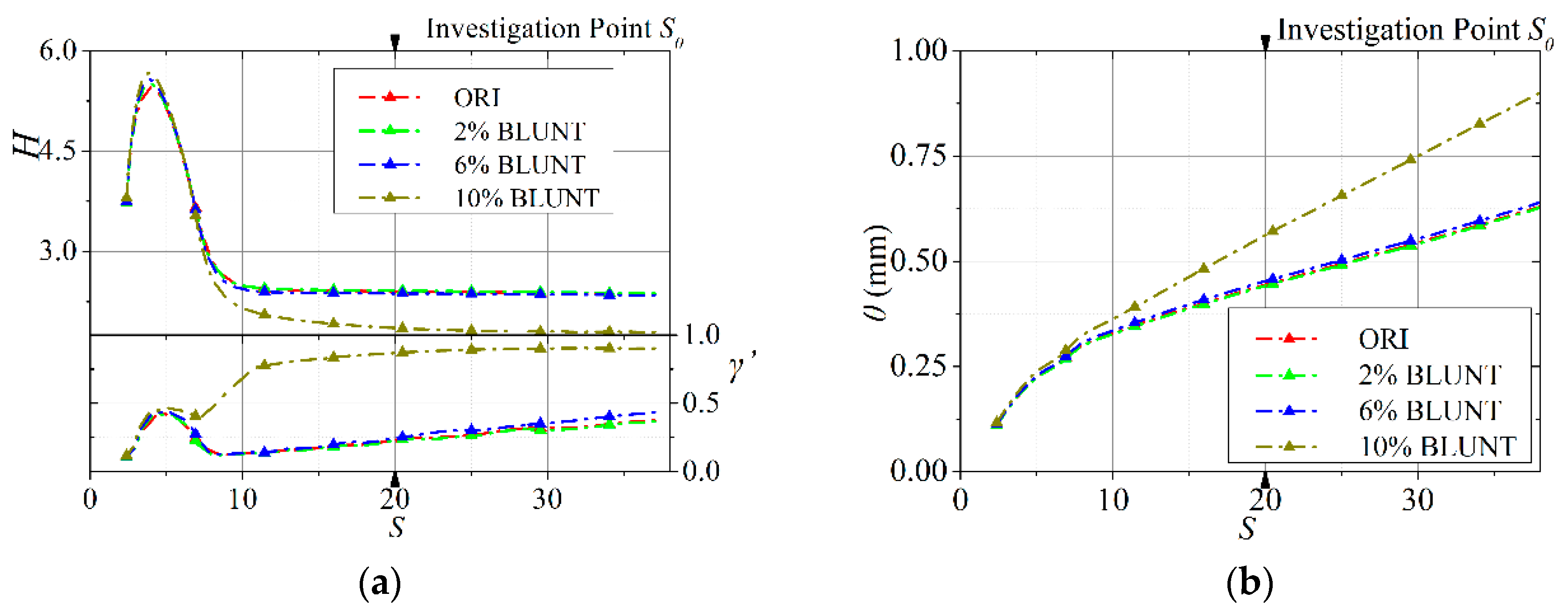
Figure 8.
The WEDGE of Ellip.LE at Tu = 5%: (a) the boundary layer shape factor and normal average turbulence intermittency; (b) the momentum thickness along aerofoils.
Figure 8.
The WEDGE of Ellip.LE at Tu = 5%: (a) the boundary layer shape factor and normal average turbulence intermittency; (b) the momentum thickness along aerofoils.

Figure 9.
The BLUNT of Ellip.LE at Tu = 7%: (a) the boundary layer shape factor and normal average turbulence intermittency; (b) the momentum thickness along aerofoils.
Figure 9.
The BLUNT of Ellip.LE at Tu = 7%: (a) the boundary layer shape factor and normal average turbulence intermittency; (b) the momentum thickness along aerofoils.

Figure 10.
The WEDGE of Ellip.LE at Tu = 7%: (a) the boundary layer shape factor and normal average turbulence intermittency; (b) the momentum thickness along the aerofoils.
Figure 10.
The WEDGE of Ellip.LE at Tu = 7%: (a) the boundary layer shape factor and normal average turbulence intermittency; (b) the momentum thickness along the aerofoils.

Figure 11.
The velocity contour near the leading edge area of the basic elliptical shape at different turbulence values: (a) At Tu = 0; (b) At Tu = 5%; (c) At Tu = 7%.
Figure 11.
The velocity contour near the leading edge area of the basic elliptical shape at different turbulence values: (a) At Tu = 0; (b) At Tu = 5%; (c) At Tu = 7%.

Figure 12.
The separation bubble modes: (a) the laminar separation/long bubble mode; (b) the laminar separation/short bubble mode; (c) the transitional separation mode.
Figure 12.
The separation bubble modes: (a) the laminar separation/long bubble mode; (b) the laminar separation/short bubble mode; (c) the transitional separation mode.

Figure 13.
The 6% BLUNT of Ellip.LE at Tu = 5%, i = 2 deg: (a) the boundary layer momentum thickness and normal average turbulence intermittency; (b) Shape factor along aerofoils.
Figure 13.
The 6% BLUNT of Ellip.LE at Tu = 5%, i = 2 deg: (a) the boundary layer momentum thickness and normal average turbulence intermittency; (b) Shape factor along aerofoils.

Figure 14.
The different leading edge shapes.

Figure 15.
The θ of different leading edges at the point of S = 50 in the low turbulence condition: (a) BLUNT series; (b) WEDGE series.
Figure 15.
The θ of different leading edges at the point of S = 50 in the low turbulence condition: (a) BLUNT series; (b) WEDGE series.

Figure 16.
θ of different leading edges at the point of S = 50 in the middle turbulence condition: (a) BLUNT series; (b) WEDGE series.
Figure 16.
θ of different leading edges at the point of S = 50 in the middle turbulence condition: (a) BLUNT series; (b) WEDGE series.

Figure 17.
The θ of different leading edges at the point of S = 50 in the high turbulence condition: (a) BLUNT series; (b) WEDGE series.
Figure 17.
The θ of different leading edges at the point of S = 50 in the high turbulence condition: (a) BLUNT series; (b) WEDGE series.

Figure 18.
The blades’ leading edge shape of ORI (ellipse) and CL-ORI (continuous curvature).

Figure 19.
The computational mesh of the cascade.

Figure 20.
The verification of the simulation: (a) Cp distribution among the suction surface at 0.5 height of CL-ORI at Tu = 2.5%, Ret = 2500; (b) Cp contour at 1.1 chord length exit.
Figure 20.
The verification of the simulation: (a) Cp distribution among the suction surface at 0.5 height of CL-ORI at Tu = 2.5%, Ret = 2500; (b) Cp contour at 1.1 chord length exit.

Figure 21.
The different leading edge boundary layer developments in the 0.5 blade height at Tu = 2.5%, Ret = 2500: (a) the boundary layer shape factor and normal average turbulence intermittency; (b) the momentum thickness along aerofoils.
Figure 21.
The different leading edge boundary layer developments in the 0.5 blade height at Tu = 2.5%, Ret = 2500: (a) the boundary layer shape factor and normal average turbulence intermittency; (b) the momentum thickness along aerofoils.

Figure 22.
The different leading edge boundary layer developments at a 0.05 blade height at Tu = 2.5%, Ret = 2500: (a) the boundary layer shape factor and normal average turbulence intermittency; (b) the momentum thickness along aerofoils.
Figure 22.
The different leading edge boundary layer developments at a 0.05 blade height at Tu = 2.5%, Ret = 2500: (a) the boundary layer shape factor and normal average turbulence intermittency; (b) the momentum thickness along aerofoils.

Figure 23.
The Cp contour at 1.1 chord length exit of BLUNT and CL-WEDGE: (a) at Ret = 2500; (b) at Re t= 3500.
Figure 23.
The Cp contour at 1.1 chord length exit of BLUNT and CL-WEDGE: (a) at Ret = 2500; (b) at Re t= 3500.
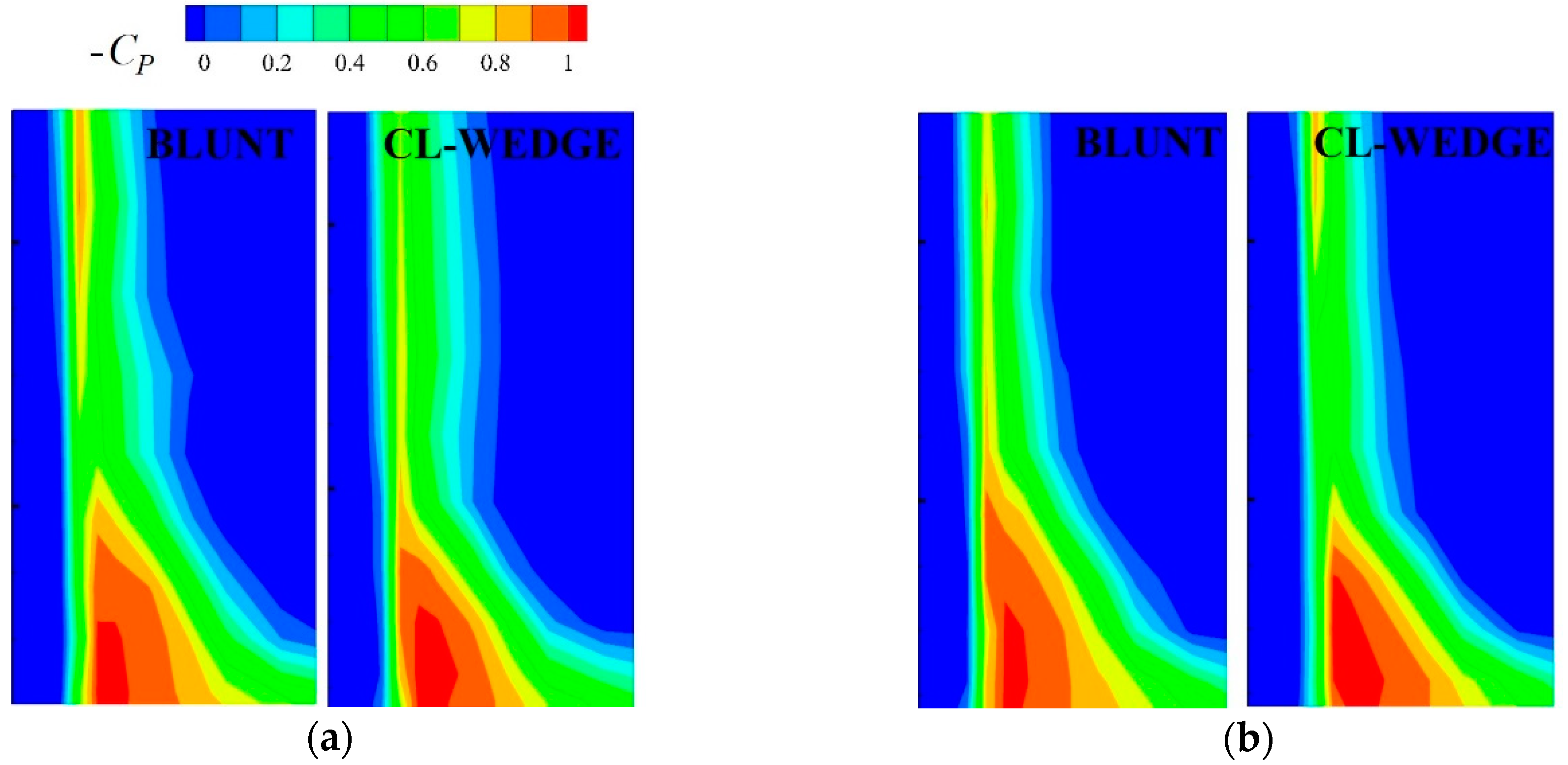
Figure 24.
The circular leading edge with a flat [44].
Figure 24.
The circular leading edge with a flat [44].


Table 1.
The physical parameters of the cascades.
| Chord Length c (mm) | Pitch t (mm) | Leading Thickness tLE (mm) | Blade Height l (mm) |
|---|---|---|---|
| 108 | 110.8 | 5.2 | 200 |
Table 2.
The leading edge deformations and naming method.
| ORI | Original elliptical leading edge shape. |
| BLUNT | Elliptical e leading edge shape with blunt deformation of ε = 2%. |
| CL-ORI | Original continuous curvature leading edge. |
| CL-WEDGE | Original continuous curvature leading edge with a wedge deformation of ε = 2%. |
© 2019 by the authors. Licensee MDPI, Basel, Switzerland. This article is an open access article distributed under the terms and conditions of the Creative Commons Attribution (CC BY) license (http://creativecommons.org/licenses/by/4.0/).
Share and Cite
MDPI and ACS Style
Li, L.; Liu, H. The Analysis of Leading Edge Deformations on Turbomachine Blades. Energies 2019, 12, 736. https://doi.org/10.3390/en12040736
AMA Style
Li L, Liu H. The Analysis of Leading Edge Deformations on Turbomachine Blades. Energies. 2019; 12(4):736. https://doi.org/10.3390/en12040736
Chicago/Turabian StyleLi, Le, and Huoxing Liu. 2019. "The Analysis of Leading Edge Deformations on Turbomachine Blades" Energies 12, no. 4: 736. https://doi.org/10.3390/en12040736
Note that from the first issue of 2016, this journal uses article numbers instead of page numbers. See further details here.