1. Introduction
As a low carbon and eco-efficient energy resource, natural gas has become an energy option to mitigate the environmental impacts of traditional fossil fuels for human beings. Natural gas is one of the most important energy resources in the world, and it fulfils more than one-fifth of energy demand worldwide [
1]. Nowadays, natural gas is extensively used for residences, commerce, transportation, electric power, and industrial production. Natural gas price forecasting is increasingly playing an essential role for stakeholder groups highly sensitive to price fluctuation [
2]. The forecast has widespread applications in all walks of life. Accurate natural gas price forecasting of one, three, five, or more months into the future is extremely significant in energy management, economic development, and environmental conservation.
Most of the international natural gas trade requires pipelines or ships for transport, because of the regional division of natural gas production and consumption. Some natural gas price systems with obvious regional characteristics have been formed around the world on account of geographical restrictions and freight rates. There are four representative prices including Henry Hub price in the United States, Average Import Cost Insurance and Freight (CIF) price in Germany, National Balancing Point (NBP) natural gas price in the United Kingdom, and Liquefied Natural Gas (LNG) price in Japan. From the perspective of pricing mechanism, North America and Britain carry out market pricing through the interplay of supply and demand gas-on-gas competition (GOG). Continental Europe adopts oil price escalation (OPE), which is linked with crude oil. Japan uses LNG pricing mechanism linked to Japan Crude Cocktail (JCC) and some regions (e.g., Russia and central Asia) still adopt monopoly pricing [
3]. These pricing systems are strongly associated with natural gas trade around the world. Natural gas prices fluctuate dramatically and we take the Henry Hub natural gas spot price in the United States as an example to explain. There are several sharp price fluctuations (e.g., October to December 2005 and April to July 2008) from 2001–2009. The change of natural gas prices is basically stable except for some small fluctuations within a narrow range since 2009. The determinants of natural gas price are complex and diversified, since the natural gas market is completely deregulated and market-driven. The price suffers from various factors and parameters, e.g., other energy prices, exploration activity, and supply-demand relation. Thus, it is a challenging task to accurately forecast natural gas price.
So far, many methods have been proposed for natural gas price forecasting. By reviewing the existing work, these methods can be divided into two categories: structural models and data-driven methods. MacAvoy (2000) predicted a long-term negative trend of wellhead gas price obtained by the simulation of a partial equilibrium model of the American industry [
4]. Buchananan et al. (2001) obtained the direction of monthly natural gas spot price movements from the viewpoint of trader positions [
5]. Woo et al. (2006) established a relationship by utilizing a partial adjustment regression model to assess the trend of natural gas price in California [
6]. With the development of artificial intelligence technology (AI) and its powerful performance, the focus has gradually shifted from econometrics and AI technology. Nguyen et al. (2010) studied the prices of monthly natural gas forward products using wavelet transform and adaptive models and obtained the lowest normalized mean square error (NMSE) (the value is 0.15384) using the adaptive generalized autoregressive conditional heteroskedasticity (GARCH) with multicomponent forecast [
7]. Azadeh et al. (2012) developed a hybrid neuro-fuzzy method consisting of artificial neural network (ANN), fuzzy linear regression (FLR), and conventional regression (CR) to estimate natural gas prices of domestic and industrial sectors in Iran [
8].
Most publications focus on short-term load forecasting (STLF). For instance, Zheng et al. (2017) used a hybrid algorithm to construct an STLF model [
9], Kuo et al. (2018) introduced a high precision artificial neural networks model [
10], and Merkel et al. (2018) proposed deep neural network regression for short-term natural gas load forecasting [
11]. In recent years, there are some works with respect to short-term price forecasting in the natural gas spot market. Abrishami (2011) analyzed gas price forecasting with a hybrid intelligent framework consisting of group method of data handling (GMDH) neural networks and rule-based exert system (RES) [
12]. Compared with GMDH neural networks and multilayer feed-forward neural networks, the hybrid intelligent framework afforded better forecasting results using daily Henry Hub spot price from 2006–2010. However, some results obtained from the hybrid intelligent forecasting method are unconvincing, because they cannot be reproduced. Busse et al. (2012) studied the daily spot natural gas price in the German NetConnect market using a dynamic forecasting method and a nonlinear autoregressive exogenous model (NARX) neural network, because the used NARX method with only five factors (temperature, exchange rate, and the settlements of three major gas hubs) is slightly better than the naive NARX method [
13].
The study reported by Salehnia (2013) is one of the few studies that really forecasts the spot price in the natural gas market [
14]. Using Gamma test analysis, several nonlinear models including local linear regression (LLR), dynamic local linear regression (DLLR), and ANN models have been utilized to test spot prices (daily, weekly, and monthly) for Henry Hub from 1997–2012. They verified that the ANN models have a higher accuracy in predicting the natural gas spot prices than LLR and DLLR, whereas the ANN models are not good at forecasting market price shocks. Ceperic et al. (2017) presented a strategic seasonality-adjusted, support vector machine (SVM)-based model and some improvements to the forecasting method based on SVM [
15]. They used feature selection algorithms to generate model inputs. They investigated short-term Henry Hub spot natural gas prices using classical time series models such as naive, autoregression (AR), and autoregressive integrated moving average (ARIMA) and machine learning neural network and support vector regression (NN and SVR). They found that the gains are not necessarily apparent even though machine learning exhibits some improvements based on traditional time-series methods. According to this brief literature overview, it can be found that these methods [
12,
13,
14,
15] often showed better performance than traditional time-series methods in predicting natural gas prices.
For the above works on short-term price forecasting for natural gas spot markets, they consider small time periods, in general, no more than five years. In fact, it is easy to facilitate a short-term prediction while attaining an accurate forecasting result. However, fore-and-aft connection and influence in a long time period still exist and thus it is essential to investigate a long time period forecast. So far, few works exist in long time period price forecasting for natural gas spot markets. To this end, we consider such a prediction of natural gas spot price from 2001–2017 based on a boosting method. As a general method, boosting can improve the performance of any learning algorithm [
16,
17]. Boosting method is one of the popular ensemble learning methods used in machine learning [
18]. The advantage of the boosting method lies in combining a series of weak classifiers to generate a very important “committee,” and it can provide increasing significance to bad classification with iteration [
19,
20]. Such a simple trick provides dramatic improvements in the classification performance.
In this study, the least squares regression boosting (LSBoost) method [
21,
22], one of the most popular boosting methods, was used to address the regression problem of natural gas price forecasting. LSBoost uses the least squares as the loss criteria and thus can fit regression ensembles well to minimize the mean-squared error [
23]. According to the best of our knowledge, this is the first time the LSBoost method was applied in natural gas price forecasting. The original schema of the application is proposed. By studying the benefits of machine learning based on LSBoost prediction, the literature on gas price prediction was added. Moreover, it is shown that compared with the existing methods, LSBoost can significantly improve the prediction accuracy of natural gas price.
The rest of the paper proceeds as follows. The next section introduces three types of machine learning tools involved in this paper.
Section 3 shows data preparation and description, model validation technique, and forecasting performance evaluation criteria.
Section 4 states empirical and comparative research.
Section 5 concludes this work.
3. Datasets and Models
Prior to model construction, we make a few research preparation works, which are comprised of data preparation and description, model validation technique, and forecasting performance evaluation criteria.
3.1. Data Preparation and Description
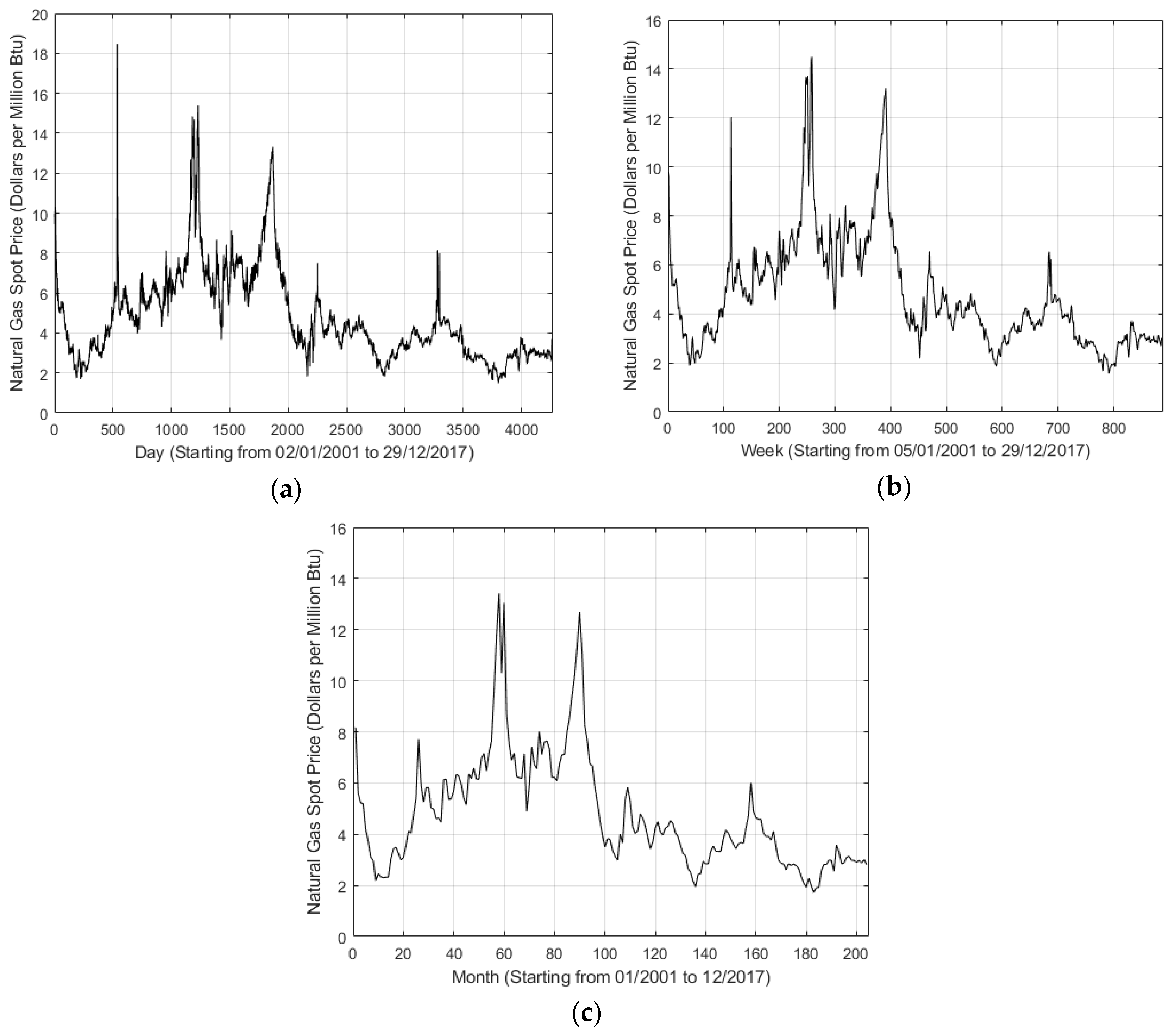
Until now, Henry Hub is not only the largest pricing point, but also the foundation for traded natural gas future contracts and other derivatives. Therefore, the historical price data of Henry Hub were selected as the observations data, and the period is from January 2001 to December 2017. This study aimed to predict the natural gas spot prices by experimentally investigating the natural gas spot price series at different frequencies, e.g., daily, weekly, and monthly. After data preprocessing, the data series of natural gas spot price includes 4260 observations of daily data, 886 observations of weekly data, and 204 observations of monthly data. In addition, there are only 4260 observations of daily data since natural gas is only traded on weekdays and some data are missing.
Figure 1 shows the daily, weekly, and monthly price trends in this period, respectively. As shown in
Figure 1, some fluctuations exist. Especially, the 537th observation in
Figure 1a shows the highest value 18.48 that occurred on 25 February 2003. Note that, for such several fluctuations, it is difficult to make a precise prediction. In addition,
Table 1 shows the descriptive statistical features of natural gas spot price series for daily, weekly, and monthly trends.
Based on Ceperic et al.’s work [
15] and Natural Gas Summary [
40], explanatory variables were obtained from the following sources: Heating Oil Prices (HO), WTI oil Prices (WTI), Baker Hughes US Natural Gas Rotary Rig Count (NGRRC), Total US Natural Gas Marketed Production (NGMP), Total US Natural Gas Consumption (NGC), Total US Natural Gas Underground Storage Capacity (NGUSC), and Total US Natural Gas Imports (NGI). The response variable is the natural gas spot price. The explanatory variables are almost associated with natural gas prices. Moreover, they demonstrate various driving factors of natural gas price to some extent. All the data collected in this study were obtained from the Energy Information Administration (EIA) website [
40].
3.2. Model Validation Techniques
Cross-validation (CV) was used to estimate the prediction accuracy to avoid overfitting [
41]. The CV is achieved by dividing the dataset into folds and estimating the accuracy on each fold with other folds as training data. As a result, the CV can obtain effective information from limited data as much as possible. The CV partitions a dataset into a training sample and validation (testing) sample. K-fold CV is a common form of CV; it randomly splits the training dataset into k subsamples of almost equal size. In this study, 10-fold CV was used, because k = 10 is widely used in practice.
3.3. Forecasting Performance Evaluation Criteria
To evaluate the forecasting performance, four statistical methods were used for measuring the forecasting errors. The methods include the following: R-square (R
2) measures the goodness-of-fit for the entire regression [
42]. The R
2 value ranges from 0–1. The closer the value is to 1, the better the goodness-of-fit of the regression line to the observed value and vice versa [
43,
44]:
where
is the actual value at the time
,
is the prediction value at the time
, and
is the number of observed data.
The mean absolute error (MAE) is a quantity to measure how close the forecasts or predictions are to the final outcomes. MAE can be expressed as follows [
45,
46]:
Mean square error (MSE) calculates the square of differences between the observed and predicted values, penalizing the highest gaps [
47,
48].
Root-mean-square error (RMSE) can well quantify large forecast errors owing to high sensitivity. Consequently, RMSE can be applied to scenarios that can tolerate smaller errors while enhancing the effect of larger errors. More details are provided in the literature [
47,
49,
50]:
In these three criteria MAE, MSE, and RMSE, the smaller values indicate the better forecasting performance of the model, because they reveal the deviation between actual and predicted values.
5. Conclusions
The goal of this study was to introduce a new machine learning approach LSBoost for natural gas price forecasting. Using seven variables including HO, WTI, NGRRC, NGMP, NGC, NGUSC, and NGI, Henry Hub natural gas spot prices starting from January 2001 to December 2017 were investigated. The LSBoost algorithm shows superiority in natural gas price prediction, because it achieved the highest R-square and lowest MAE, MSE, and RMSE compared with the existing methods such as linear regression, linear SVM, quadratic SVM, and cubic SVM. Our experiments on the datasets demonstrate that LSBoost model is superior and promising. In the future, we consider possible improvements in the proposed model based on the LSBoost method in terms of predicting performance, and we will try to extend the method and analysis presented in this study to forecast other fuel prices, such as crude oil.


