Abstract
Accurate and reliable vehicle velocity estimation is greatly motivated by the increasing demands of high-precision motion control for autonomous vehicles and the decreasing cost of the required multi-axis IMU sensors. A practical estimation method for the longitudinal and lateral velocities of electric vehicles is proposed. Two reliable driving empirical judgements about the velocities are extracted from the signals of the ordinary onboard vehicle sensors, which correct the integral errors of the corresponding kinematic equations on a long timescale. Meanwhile, the additive biases of the measured accelerations are estimated recursively by comparing the integral of the measured accelerations with the difference of the estimated velocities between the adjacent strong empirical correction instants, which further compensates the kinematic integral error on short timescale. The algorithm is verified by both the CarSim-Simulink co-simulation and the controller-in-the-loop test under the CarMaker-RoadBox environment. The results show that the velocities can be accurately and reliably estimated under a wide range of driving conditions without prior knowledge of the tire-model and other unavailable signals or frequently changeable model parameters. The relative estimation error of the longitudinal velocity and the absolute estimation error of the lateral velocity are kept within 2% and 0.5 km/h, respectively.
1. Introduction
The increasing demands for high precision motion control of autonomous vehicles has led to an urgent need for accurate and reliable vehicle state estimation, and the decreasing cost of high precision sensors, for instance, multi-axis inertial measurement units (IMUs), also motivates this effort [1]. Although accurate and reliable velocity estimation is a general research issue for all kinds of vehicles, it is particularly attractive for electric vehicles. Since the motors have more accurate and rapid torque response than internal-combustion engines, the electrification of vehicles has greatly improved the performance potential of the vehicle control systems, including the energy management systems [2], the regenerative braking systems [3], the anti-slip control systems [4], etc. These advanced vehicle control systems depend deeply on accurate and reliable feedback of the vehicle velocity. The topic of vehicle state estimation is traditional, but never out of date, as some of the main difficulties are still haunting the whole vehicular industry [5]. Theoretically, when a vehicle is mounted with a 6-axis IMU, the vehicle velocities can be obtained using the integral of the measured accelerations and angular speeds, however, this thoroughly kinematic-dependent method is not applicable due to several critical reasons. Firstly, most commercial vehicles are mounted with a 3-axis IMU instead of 6-axis IMU, and generally only the yaw rate and the longitudinal and lateral accelerations are measured, which is not enough for determining the 6-DOF motion information of the vehicle body. Secondly, the measured accelerations are coupled with the gravity and the body’s attitude, and the velocities cannot be estimated independently of the attitude estimation [6]. Thirdly and most importantly, the existence of biases and noises of the measured kinematic signals will introduce divergent or unacceptable integral error in the estimated velocities [7,8,9]. To solve these problems, the kinematics-based estimation results are generally corrected by fusing with extra measurements such as GPS or integrating a vehicle dynamics model. In terms of the influence of the tire-model, these correction methods can be divided into tire-model-based and non-tire-model-based methods.
Regarding the tire-model-based methods [5,6,7,8,9,10,11,12], the measured kinematic signals can be corrected by the vehicle dynamics equations provided that the tire forces are estimated by particularly designed observers. Various tire-models can be used, including analytical models like linear model [12], Dugoff’s model [13], LuGre tire-model [14,15], etc., and semi-empirical models like Pacejka’s tire-model [16], the UniTire model [17], etc. For instance, in [1], a corner-based vehicle state estimator combing the lumped LuGre tire-model and the vehicle kinematics is proposed. In [5], to reduce the impact of the arbitrary nonlinear tire-model error, a minimum model error criterion-based algorithm combining with the extended Kalman filter is proposed, and the algorithm manages to show robustness against limited tire-model errors. In [6], a combination of the kinematics-based model and the inverse LuGre tire-model is used to estimate longitudinal and lateral vehicle velocities. In [11], a combination of kinematics- and model-based approaches with a linear tire-model is used to estimate vehicle sideslip angle. The drawbacks of the tire-model-based methods are obvious and fatal. Firstly, the tire-model parameters are generally unavailable and frequently changeable with the road conditions and the tire aging. Secondly, most tire models need the feedback of the estimated vehicle velocities, which introduces the algebraic loop and the risk of numerical instability. Thirdly, even if the tire forces are accurately estimated, the dynamics-based algorithm still needs the vehicle inertia parameters, the road gradient and bank angles, and the air-drag resistances, etc. to construct reliable dynamics equations for correction, and these parameters are also time-varying and hard to obtain.
Regarding the non-tire-model-based methods [18,19,20,21,22,23,24,25,26,27], the main idea is to use other measured information apart from the IMU signals to complete a fused estimation of the vehicle state. Typically, the global positioning system (GPS) is used, and a combination of GPS and IMU gives satisfactory estimation results [18,19,20,21,22,23,24]. For instance, Farrell et al. [21] used the carrier-phase differential GPS to increase the accuracy of the estimated heading and position. Bevly et al. [22,23] used accurate GPS to remove noises and address the low excitation scenarios using some kinematic-based methodologies. Yoon et al. [24] utilized two low-cost GPS receivers for the lateral velocity estimation and compensated the low update rate issue of conventional GPS receivers by combining the IMU and GPS data. Mathematically, there are various techniques for fusing the IMU signals with the GPS data, including Kalman-filter-based methods [25,26], nonlinear observers [27,28], etc. Apart from the GPS, other extra measurements such as tire-force sensor [29,30], wheel speed encoder, radar or camera data can also be introduced for vehicle state estimation. For instance, in [31,32], the vehicle longitudinal velocity is estimated by using an accelerometer and wheel encoders. An adaptive non-linear filter method [33] is another empirical approach to estimate vehicle velocity by using information from wheel velocities. These non-tire-model-based methods are attractive, but some drawbacks still exist. Firstly, the introduction of new measurements like GPS brings high cost and reception may be lost in some areas. In addition, it is difficult to solve the problem of weight distribution among different measured signals.
Based on the multi-axis IMU and other ordinary on-board vehicle sensors, we propose a non-tire-model-based estimation method for the vehicle velocities without extra measurements such as GPS. Based on the available sensor signals, some reliable empirical judgments about the vehicle velocities can be extracted. The core innovative idea is to use these empirical judgments to correct the vehicle velocities that are obtained by the kinematic integral of the IMU signals on a long timescale. Meanwhile, the additive biases of the measured accelerations can be estimated recursively by comparing the integral of the measured accelerations with the difference of the estimated velocities between the adjacent strong empirical correction time instants. Owing to the recursively compensated biases, the integral error of the kinematics equations can be further restrained on a short timescale. To sum up, by taking full advantage of the reliable empirical judgments about the vehicle velocities, we attempt to correct the integral error of the thoroughly kinematic-based vehicle velocities estimation results on both long and short timescales. The main advantages of the proposed estimation algorithm are listed as follows:
- (1)
- The algorithm is neither tire-model-based nor GPS-dependent, and it does not involve any other model parameters such as the inertia parameters, the mass centroid location, and the road adhesion conditions, etc.
- (2)
- The algorithm is applicable for a wide range of driving conditions, since the kinematics equations are independent of the driving maneuvers, and the empirical judgement about the velocities also widely holds.
The paper is organized as follows: Section 2 describes the estimation problem and the overall scheme. Section 3 introduces the estimation algorithms in detail. In Section 4, simulation tests are carried out to verify the algorithm. In Section 5, the controller-in-the-loop test is carried out to verify the algorithm under real time condition. Section 6 concludes this paper.
2. Problem Description and the Overall Scheme
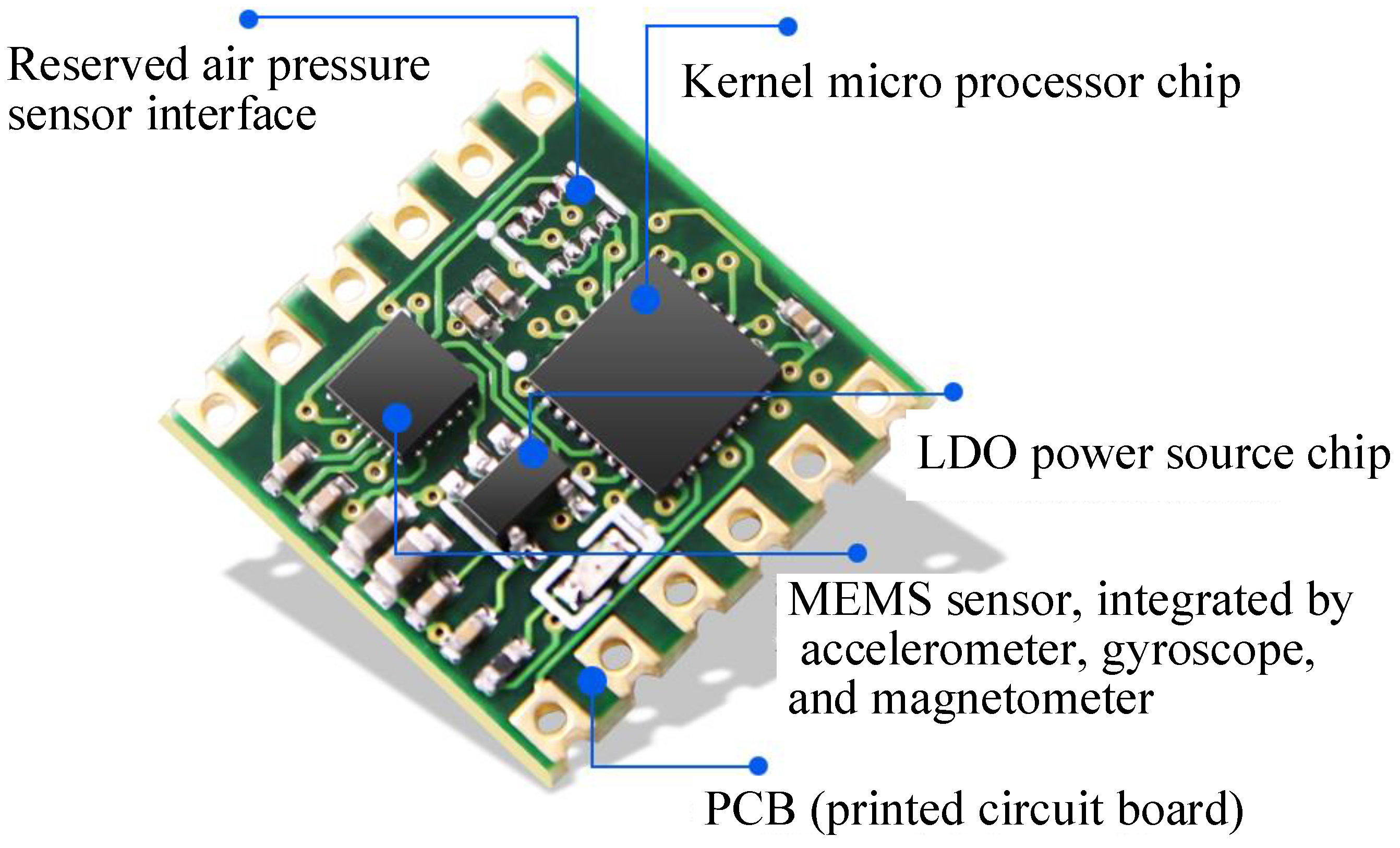
This paper attempts to provide a complete and practical estimation solution for the longitudinal and lateral velocities with the multi-axis IMU and other ordinary on-board vehicle sensors. The velocities at the mounting point of the IMU in its body-fixed coordinate system are the reference estimation targets. The ordinary on-board vehicle sensors include the wheel speed encoders and the angular sensor of the steering wheel. The multi-axis IMU is the key sensor that makes the non-tire-model-based vehicle velocities estimation possible. It is integrated by a 3-axis accelerometer, a 3-axis gyroscope, and a 3-axis magnetometer, which measures the 3-dimensional accelerations, angular speeds, and attitude angles respectively. Figure 1 and Table 1 demonstrates an example of the integrated multi-axis IMU chip and its key technical indexes respectively, which costs about $15 US.

Figure 1.
The integrated multi-axis IMU chip.

Table 1.
The key technical indexes of the multi-axis IMU chip.
The estimation algorithm should not be tire-model-based for practicability. Furthermore, the algorithm should not depend on any prior knowledge of other unavailable or frequently changeable parameters, such as the sprung-mass and its centroid location, the rolling resistance, the air-drag coefficients, etc. The dependable signals and parameters include: (1) the 3-dimensional accelerations, angular speeds, and attitude angles measured by the multi-axis IMU; (2) the wheel speeds; (3) the angle of the steering wheel; (4) the effective rolling radius of the wheels. Apart from the available signals and parameters, some critical and reasonable assumptions should also be clarified, including: (1) the attitude of the IMU is mounted in accordance with the sprung mass’s body-fixed coordinate system; and (2) the measuring errors of the accelerations are modeled as a summation of a relatively fixed additive bias and the white Gaussian noise.
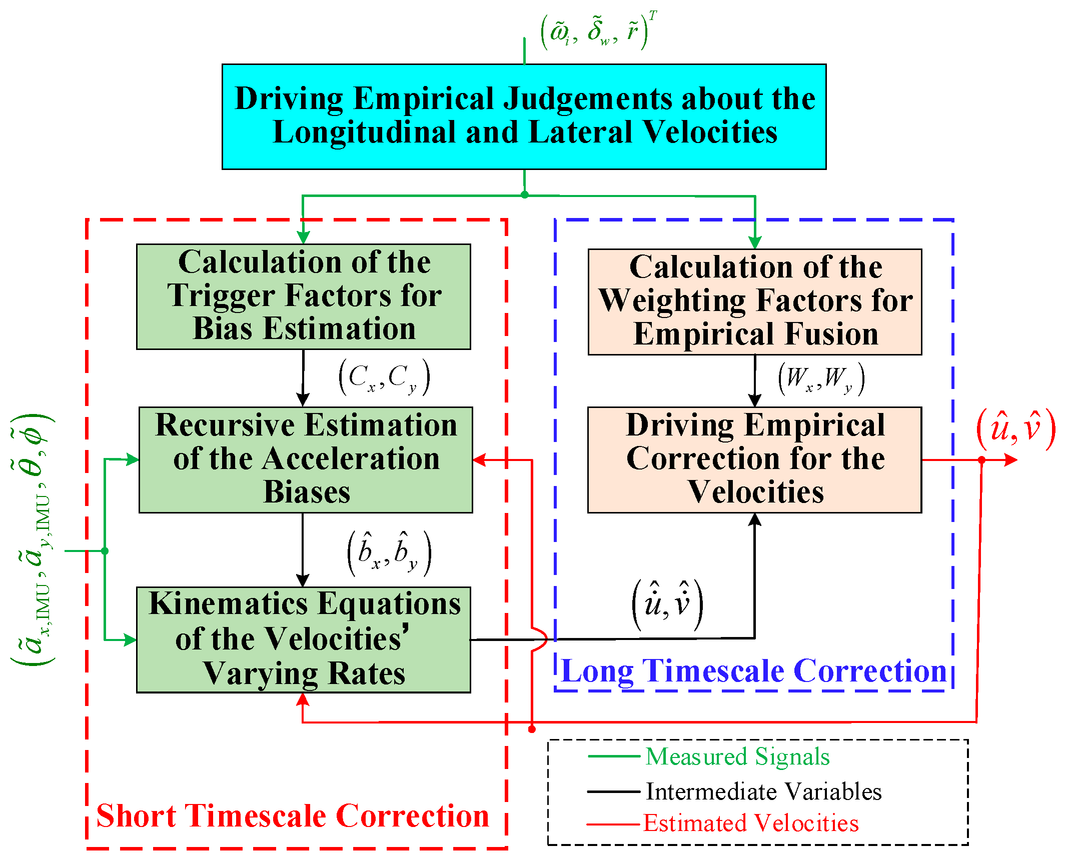
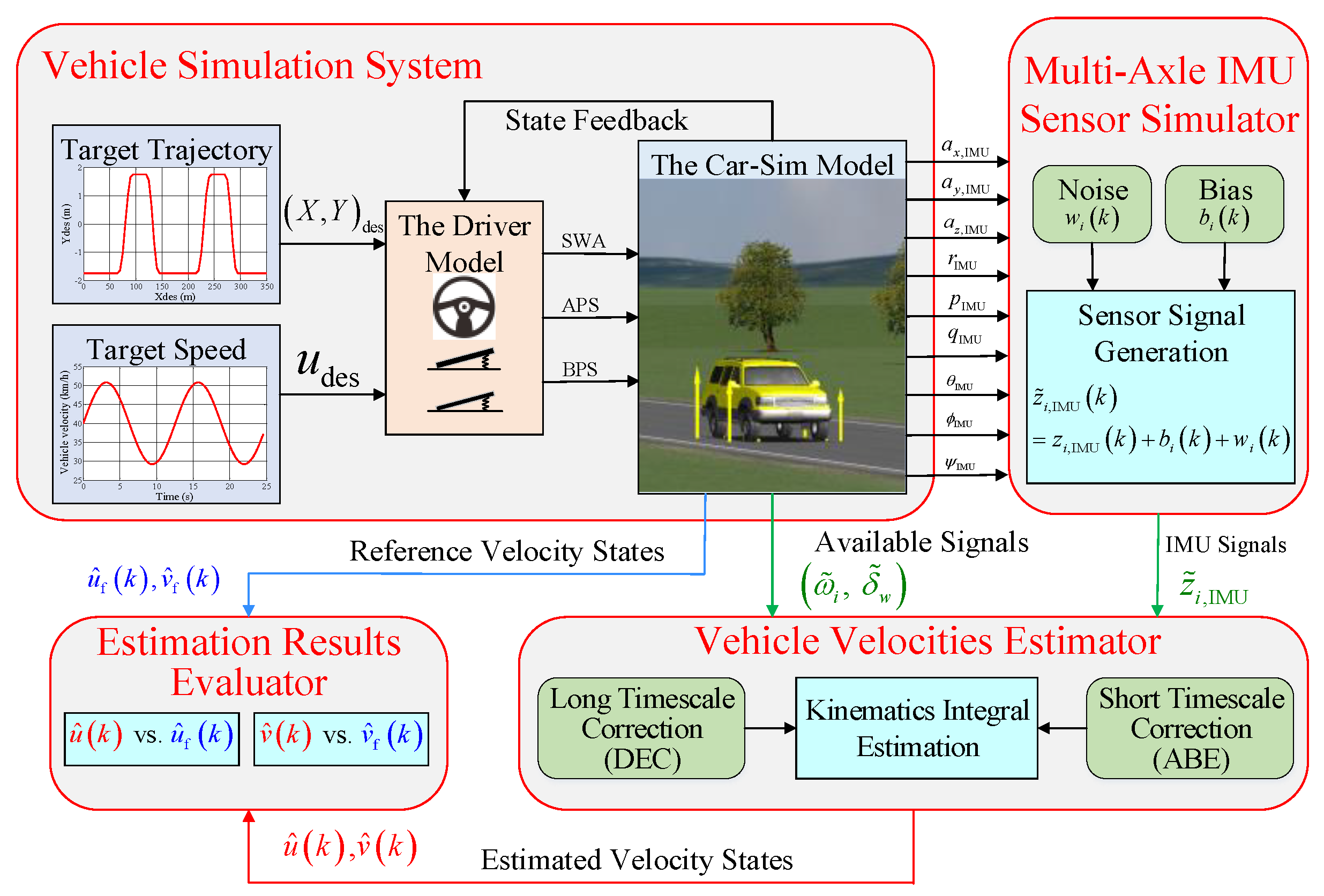
The overall scheme of the estimator is shown in Figure 2. Firstly, the driving empirical judgements about the longitudinal and lateral velocities are extracted from the wheel speeds , the yaw rate , and the steering wheel angle . On top of that, an integrated estimation framework fusing with the driving empirical correction (DEC) and the acceleration bias estimation (ABE) is proposed to correct the integral errors of the kinematics equations on both long and short timescales. In Figure 2, are the estimated longitudinal and lateral velocities, are the measured longitudinal and lateral accelerations, are the measured Euler pitch and roll angles. are the estimated biases of the measured accelerations. Wx, Wy are the weighting factors for fusing the driving empirical judgements with the longitudinal and lateral kinematics integral equations respectively, Cx, Cy are the trigger factors for updating the estimation of the longitudinal and lateral acceleration biases respectively. In this paper, we use accents “~” and “^” to represent the measured and estimated values, respectively.

Figure 2.
The overall scheme of the estimator.
3. Estimation Algorithm for the Velocities
3.1. The Kinematics Integral Equations
Nominate the Euler yaw angle, pitch angle and roll angle of the sprung-mass as respectively. Three rotation transformation matrices are noted as:
The measured accelerations can be represented as:
where are the measured accelerations of the IMU. ai,O are the theoretical accelerations at the measuring point without the influence of gravity. gi are the components of the acceleration of gravity, bi and wi represent the biases and noises of the sensor, respectively.
In Equation (2), gi can be deduced as:
According to the kinematics equation of the rigid body, the theoretical accelerations at the measuring point is described as:
where are roll rate, pitch rate, and yaw rate of the body respectively. are the longitudinal, lateral and vertical velocities respectively.
Combining (2)–(4), we have:
By ignoring the vertical vibration of the vehicle, according to Equation (5), we have:
Thus, the estimated varying rates of the longitudinal and lateral velocities at the measuring point can be formulated as:
Equation (7) is a kinematics-based equation, and it does not rely on any vehicle or tire-model parameters. Theoretically, the vehicle velocities can be directly estimated by the integral of Equation (7). However, this method is critically restricted due to the existence of the unknown biases and noises of the measured acceleration, which generates unacceptable accumulative kinematics integral error. This involves the DEC on long timescale and the ABE on short timescale, which act as the core innovative algorithms for improving the estimation accuracy of the velocities in this paper.
3.2. The Estimation of the Euler Angles
It should be noted that as the measured accelerations are coupled with the attitude angles due to the existence of gravity, the components of gravity acceleration should be isolated from the measured acceleration signals in Equation (7), which involves the real-time estimation of the Euler pitch and roll angles. Owing to the use of the multi-axis IMU exemplified in Figure 1, the Euler angles can be estimated by fusing the attitude angles measured by the 3-axis magnetometer and the angular speeds measured by the 3-axis gyroscope, and the fusion algorithms are commonly Kalman-filter-based. The discretized Euler angle estimation system including the state transition equation and the observation equation are listed as follows:
where x(k) is the state vector to be estimated, u(k) is the input vector measured by the gyroscopes, z(k) is the observation vector measured by the magnetometer, w(k) and v(k) denotes the noise of the state transition equation and the observation equation respectively, Ts is the communication period of the estimator, normally Ts = 20 ms. B(x(k)) is the time-varying input matrix related to the state vector itself, which is given as:
Equation (8) defines a discrete linear time-varying estimation system with a unit system matrix (A = I) and output matrix (C = I). For such special estimation system, the Kalman filtering estimation algorithm is described as follows:
where Q and R denote the covariance matrixes of the measured angular velocities and the attitude angles, respectively, which can be set according to the error indexes of the IMU shown in Table 1.
Typically, the fusion estimation algorithm of the gyroscopes and the magnetometers given by Equation (10) is embedded in the kernel microprocessor chip shown in Figure 1. Therefore, in Equation (7), the eventually output Euler pitch and roll angles of the IMU chip are the fusion results of all the directly measured angles and angular speeds. The accuracy of the output Euler angles can generally reach 0.05 deg and 0.1 deg under static and dynamic conditions, respectively, as shown in Table 1. Thus, the estimation of the Euler angles is not performed in the vehicle state estimator of the vehicle control unit (VCU). The reliable and accurate attitude output of the multi-axis IMU is one of the significant premises that makes the kinematics-based estimation algorithm realizable.
3.3. Driving Empirical Judgements
Apart from the kinematics equations given by (7), some practical reliable judgments about the longitudinal and lateral vehicle velocities can be extracted directly from the ordinary measured signals such as the wheel speeds, the steering wheel angle and the yaw rate under particular conditions. These empirical judgements can be wisely used to correct the accumulative errors introduced by the direct integral of the measured accelerations in both long and short timescales. Two empirical judgements about the longitudinal and lateral velocities are summarized as follows:
Experience 1: When the wheel speeds are basically the same, at the instant when the average varying rates of the speeds crosses zero, the vehicle is generally at the critical point between driving and braking. At this moment, the slip ratio of the tire is approximately zero, and the longitudinal vehicle velocity can be estimated with enough accuracy as the product of the average wheel speed and the effective rolling radius.
Experience 2: When the angle of the steering wheel and the yaw rate remain around zero for a considerable range of time, the vehicle is generally driving straight in the longitudinal direction. During this situation, the lateral vehicle velocity can reliably be estimated as zero.
3.4. Driving Empirical Correction
Based on the Experiences 1 and 2, the DEC method is proposed to correct the accumulative errors introduced by the direct integral of the measured accelerations at appropriate time instants on long timescale.
3.4.1. DEC for the Longitudinal Velocity
According to Experience 1, the empirical wheel-speed-based correction of the longitudinal velocity is proposed as follows:
where Reff is the effective rolling radius, is the average wheel speed, Wx is the weighting factor for fusing Experience 1 with the longitudinal kinematics integral equation, which is calculated as:
where , are the relative variance scales of the wheel speeds and their average varying rates respectively, smaller and indicate stricter judgement condition for Experience 1, are the measured wheel speeds, and the average wheel speed and the their average varying rate are calculated as follows:
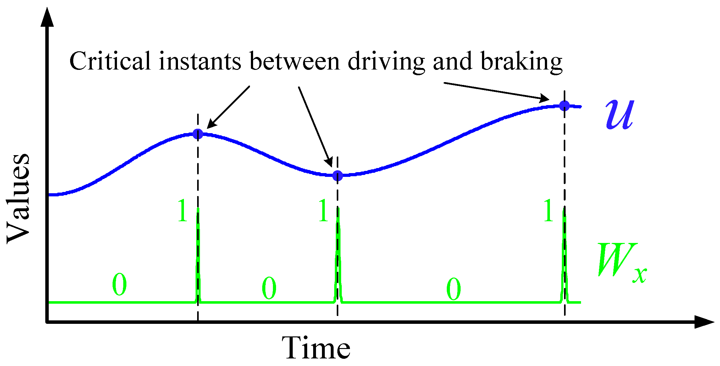
In summary, according to Equation (11), when the wheel speeds are close to each other and their average variation rate is small, Wx approaches 1, and the estimated longitudinal velocity relies mostly on the average wheel speed. On the contrary, when Wx approaches 0, and the estimated longitudinal velocity relies mainly on the kinematic integral of the estimated varying rates of the longitudinal velocity given by Equation (7). Figure 3 demonstrates the varying characteristic of Wx with the varying longitudinal velocity. By appropriately choosing small parameters and , it can be imagined that Equation (11) performs necessary and reliable correction for the integral error of the longitudinal velocity on long timescale at the critical point between driving and braking.

Figure 3.
The value of Wx with varying longitudinal velocity.
3.4.2. DEC for the Lateral Velocity
According to Experience 2, the empirical straight-driving-based correction of the lateral velocity is proposed as follows:
where Wy is the weighting factor for fusing Experience 2 with the lateral kinematic integral equation, which is calculated as:
where is a scale value used to measure the time range of the empirical straight-driving. ty is a timer used to record the continuous empirical straight-driving time, it can be accumulated or reset according to the steering wheel angle and the yaw rate, given as:
where is the measured steering wheel angle, rth and δw,th are small threshold values.
In summary, according to Equation (14), when the measured steering wheel angle and the yaw rate maintain around zero for a considerable range of time, Wy approaches 0, and the estimated lateral velocity will be driven to zero rapidly. On the contrary, Wy maintains at 1, and the estimated lateral velocity relies mainly on the kinematic integral of the estimated varying rates of the lateral velocity given by Equation (7).
Figure 4 demonstrates the varying characteristic of Wy with the varying lateral velocity. By choosing small parameters , rth and δw,th appropriately, it can be imagined that Equation (14) performs necessary and reliable correction for the integral error of the lateral velocities on long timescale when the vehicle is driving straightly.
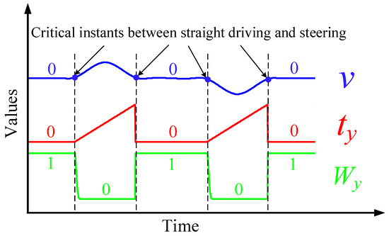
Figure 4.
The value of Wx with varying lateral velocity.
3.5. Acceleration Bias Estimation
As described by Equations (11) and (14), the DEC methods generate accurate and reliable corrections for the estimated velocities when the driving experiences are satisfied occasionally on long timescale. However, in most time intervals, the estimation accuracy depends mainly on the kinematic integral errors of Equation (7), which is critically influenced by the unknown biases of the measured accelerations, namely bx and by. Fortunately, by comparing the integral of the measured accelerations with the difference of the estimated velocities between the adjacent strong empirical correction time instants, the recursive estimation of the accelerations’ biases can be realized. With the recursively updated biases, Equation (7) can generate more accurate estimation of the velocity varying rates, which in turn improves the accuracy of the integral estimation of the velocities on short timescale.
3.5.1. Estimation of the Longitudinal Acceleration Bias
According to Equations (11)–(13), every time when Wx approaches 1, the longitudinal velocity can be well estimated by the average wheel speed. Thus, the difference of the longitudinal velocity between the adjacent strong DEC points tx0,txf when Wx approaches 1 can be easily calculated. Meanwhile, the integral of the estimated varying rate of the longitudinal velocity within the same time interval [tx0,txf] can also be recorded by the estimator. We can use the difference between them to estimate the bias of the measured longitudinal acceleration recursively. The algorithm is deduced as follows:
From the above equation, we get:
where:
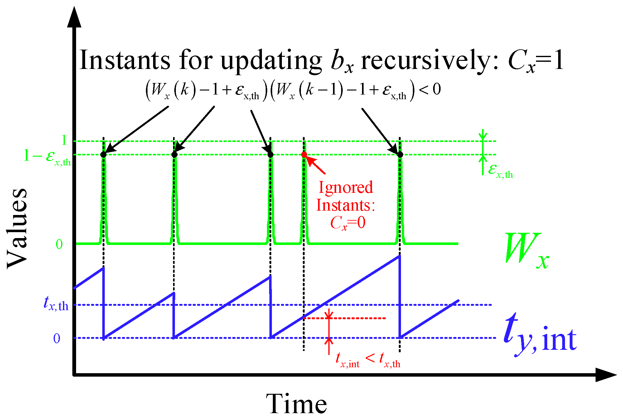
The trigger condition for activating a new round of recursive estimation of bx is designed as:
where εx,th is a small positive threshold value, tx,int is the current timer value which records the time range since the last time when the estimator of bx was triggered, tx,th represents the least effective integral time range for getting rid of the influence of the longitudinal measuring noise. The trigger condition (20) for the recursive estimation of bx is further demonstrated by Figure 5.
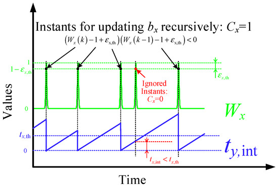
Figure 5.
The instants for updating bx recursively.
When Cx = 0, the timer of tx,int works, and the integral part of Equation (18), noted as ub,0f, accumulates. The estimated bias remains the same. The algorithm is formulated as:
When Cx = 1, the empirical final velocity is updated according to the current average wheel speed, then the RLS-F algorithm is used to generate a new round estimation of , after that, tx,int and ub,0f are reset as zero, and the empirical initial velocity is reset as the current final empirical velocity , preparing for the next round estimation of .The RLS-F algorithm represents the recursive least square algorithm with forgetting factor. In this paper, the RLS-F algorithm is repeatedly used for estimating the parameters with time-invariant or slow time-varying characteristics. In summary, when Cx = 1, the algorithm is formulated as follows:
The forgetting factor, the initial bias and its covariance for estimating bx are recommended as:
where , Px,f are the final iterative value during the last driving process, which is saved in the flash memory of the VCU every time before switching off. In our study, the values are set as = 0, Px,f = 0.02 for testing.
It should be emphasized that the updated is timely returned to Equation (7) for improving the estimation accuracy of on short timescales.
3.5.2. Estimation of the Lateral Acceleration Bias
According to Equations (14)–(16), every time Wy approaches or leaves from zero, the vehicle is at the critical point between straight driving and steering, and the lateral velocity can be reliably estimated as zero. Thus, the difference of the lateral velocity between the adjacent strong DEC point ty0,tyf when Wy approaches or leaves from zero is approximately zero. Meanwhile, the integral of the estimated varying rate of the lateral velocity within the same time interval [ty0,tyf] can also be recorded by the estimator. We can use the difference between them to estimate the bias of the measured lateral acceleration. The algorithm is deduced as follows:
From the above equation, we get:
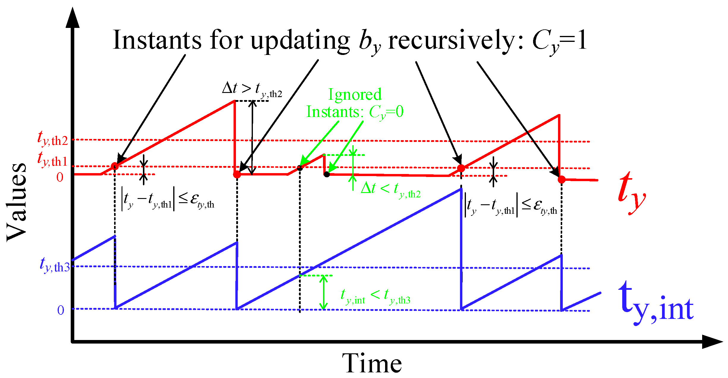
The trigger condition for activating a new round of recursive estimation of by is designed as:
where condition |ty − ty,th1| < εty,th represents the instant when the vehicle turns to straight driving from steering, condition ty(k − 1) − ty(k) > ty,th2 represents the instant when the vehicle turns to steering from straight driving. ty,th1 and εty,th are small threshold values, ty,th1 is much greater than εty,th, and ty,th2 is much greater than ty,th1. ty,int is the current timer value which records the time range since the last time when the estimation of by was triggered, ty,th3 represents the least effective integral time range for getting rid of the influence of the lateral measuring noise. The trigger condition (26) for the recursive estimation of by is further demonstrated by Figure 6.
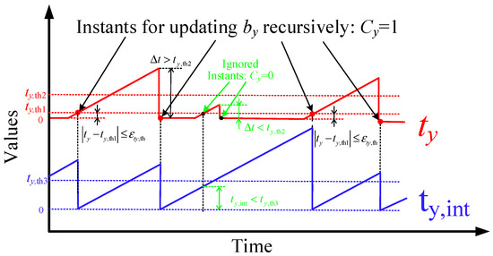
Figure 6.
The instants for updating by recursively.
When Cy = 0, the timer of ty,int works, and the integral part of Equation (25), noted as vb,0f, accumulates. The estimated bias remains the same. The algorithm is formulated as:
When Cy = 1, the RLS-F algorithm is activated to generate a new round estimation of , next, ty,int and vb,0f are reset as zero for the next round estimation of . The algorithm is summarized as:
The forgetting factor, the initial bias and its covariance for estimating by are recommended as:
where , Py,f are the final iterative value during the last driving process. In our study, the values are set as = 0, Py,f = 0.02 for testing.
Similar to , the updated is timely returned to Equation (7) for improving the estimation accuracy of on a short timescale.
4. Carsim-Simulink Co-Simulation Analysis
4.1. The Simulation Platform
To evaluate the performance of the proposed estimation algorithm, a simulation platform is established with CarSim combining with Simulink [34], as shown in Figure 7. The platform includes four subsystems: (1) the vehicle simulation system; (2) the multi-axis IMU sensor simulator; (3) the vehicle velocities estimator; (4) and the estimation results evaluator.
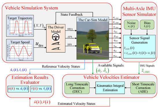
Figure 7.
The CarSim-Simulink Co-simulation platform.
The vehicle simulation system is established in CarSim. The demo car is a four-wheel-independently motor-driven electric vehicle, and Table 2 lists the specifications of the simulated electric vehicle. The vehicle follows a specified path with the pre-defined varying target speed, driven by the driver model. In the multi-axis IMU sensor simulator, the ideal IMU signals with the influence of the gravity are extracted from the vehicle simulation system, and reasonable noises and biases are added to these ideal values according to Table 1 for simulating the real sensor signals.
Table 2.
The specifications of the simulated electric vehicle.
Using the simulated IMU signals, the wheel speeds and the steering wheel angle, the vehicle velocities estimator performs an estimation algorithm fusing with the kinematic integral and the empirical correction on both long and short timescales, which is the focus of this paper. Eventually, the estimated velocities are compared with their reference values to evaluate the algorithm.
The parameters related to the estimation algorithm are recommended in Table 3 for the simulated vehicle platform. The only vehicle parameter needed by the estimation algorithm is the effective rolling radius, which is 0.331 m in our case.
Table 3.
Recommended parameters of the estimation algorithm.
4.2. Consecutive Double-Lane-Change Test with Varying Speed
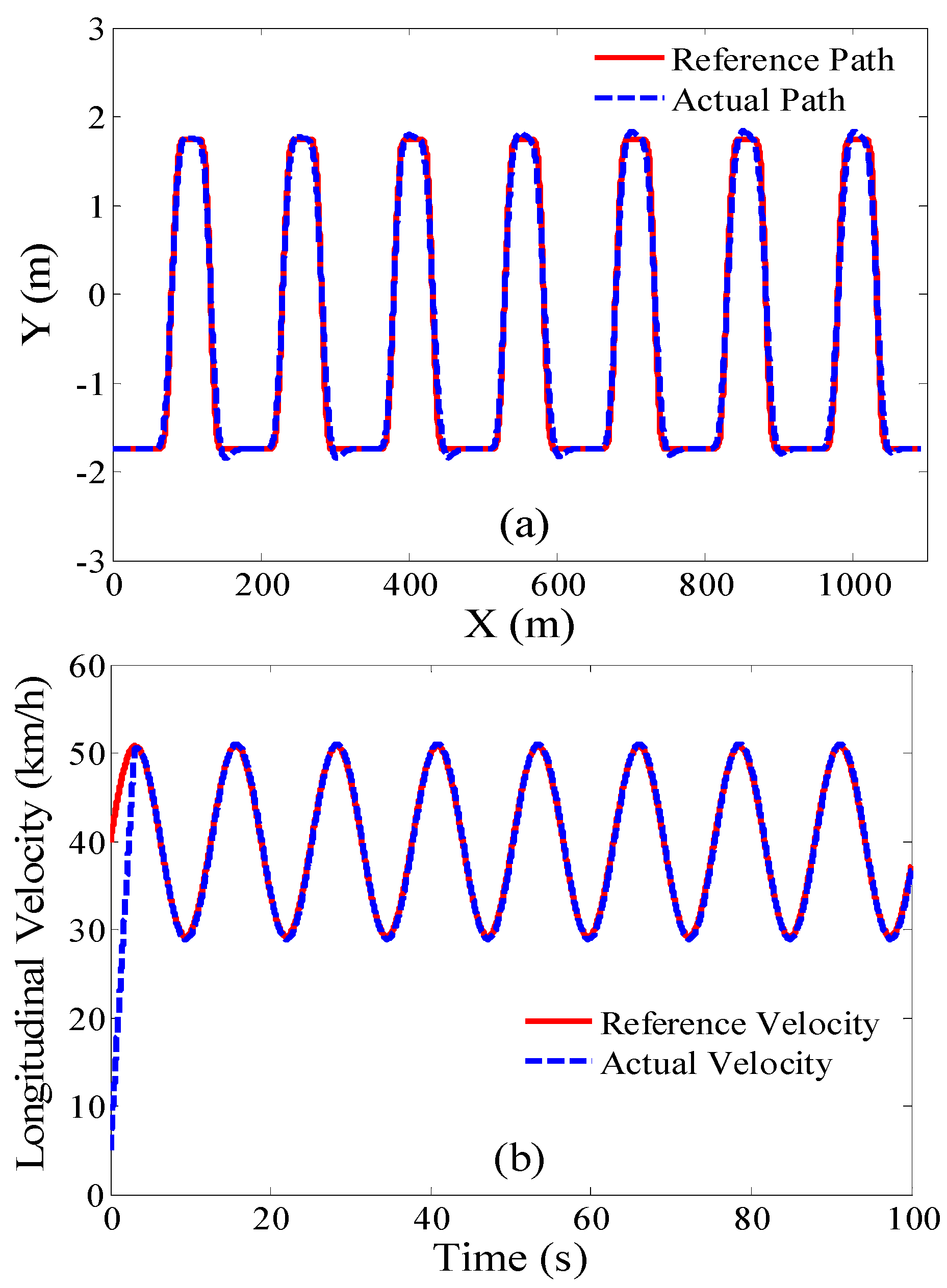
A consecutive double-lane-change (DLC) process with varying speed is tested. The initial speed is set as 5 km/h, and a sinewave varying speed with a frequency of 0.5 rad/s, amplitude of 10 km/h and average speed of 40 km/h is designed as the target speed. In addition, the biases of the measured longitudinal and lateral accelerations are set as 0.02 m/s2 and −0.02 m/s2, respectively. The road has a constant gradient of 3 deg, and the adhesion coefficient is set as 0.6. It should be noted that even though a specified road adhesion coefficient is claimed for simulation, the estimation algorithm does not need this information since the algorithm is non-tire-model-based, and the kinematics equations and the driving empirical judgements about the velocities are also independent of the road adhesion condition. Furthermore, no other information, such as the tire-model, the rolling resistance, the air-drag coefficients, and the moment inertia of the wheel, etc. are required, which makes the proposed algorithm practically applicable. The path tracking and speed following results performed by the driver model are shown in Figure 8a,b, respectively. It is shown that a 7-consecutive DLC process with a sinewave varying speed is perfectly tracked, thus a reasonable driving process is generated for testing the estimation algorithm.

Figure 8.
Tracking results of the consecutive DLC test: (a) path tracking result; (b) speed following result.
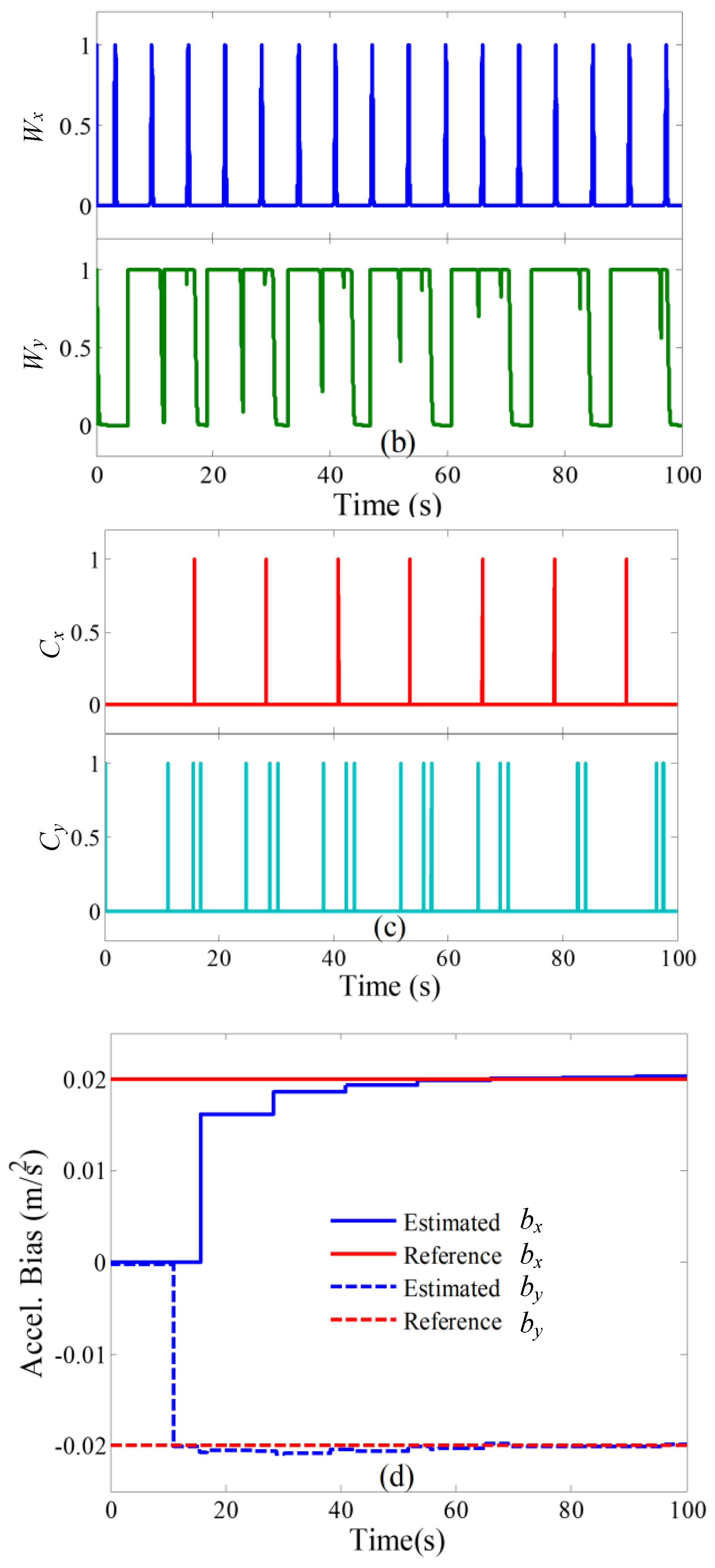
Figure 9 demonstrates the main intermediate simulation results during the consecutive DLC test. In Figure 9a, the longitudinal integral timer accumulates and resets periodically in coordinating with the sine-wave varying speed. The lateral timer accumulates in steering intervals and maintains at zero in straight driving intervals, as formulated by Equation (16). In Figure 9b, the weighting factors for the DCE indicate the desired correction action for the estimated velocities at appropriate time instants or intervals when the driving empirical judgements hold. In Figure 9b, the trigger coefficients for the ABE are waked up every time when the activation conditions for a new round of estimation of the acceleration biases hold.
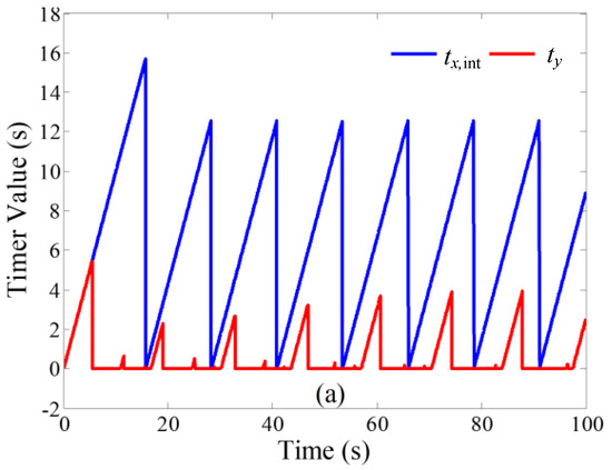
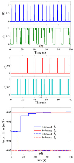
Figure 9.
Intermediate estimation results during the consecutive DLC test: (a) integral timers; (b) weighting factors for DEC (c) triggering factors for ABE; (d) acceleration biases.
Figure 9d shows that the pre-defined longitudinal and lateral biases of the measured accelerations are eventually identified. Due to the initial setting errors, it takes some time for the RLS-F algorithm to converge. After a self-learning process, satisfactory identification accuracy of the acceleration biases are obtained at approximately the end of the third DLC process.
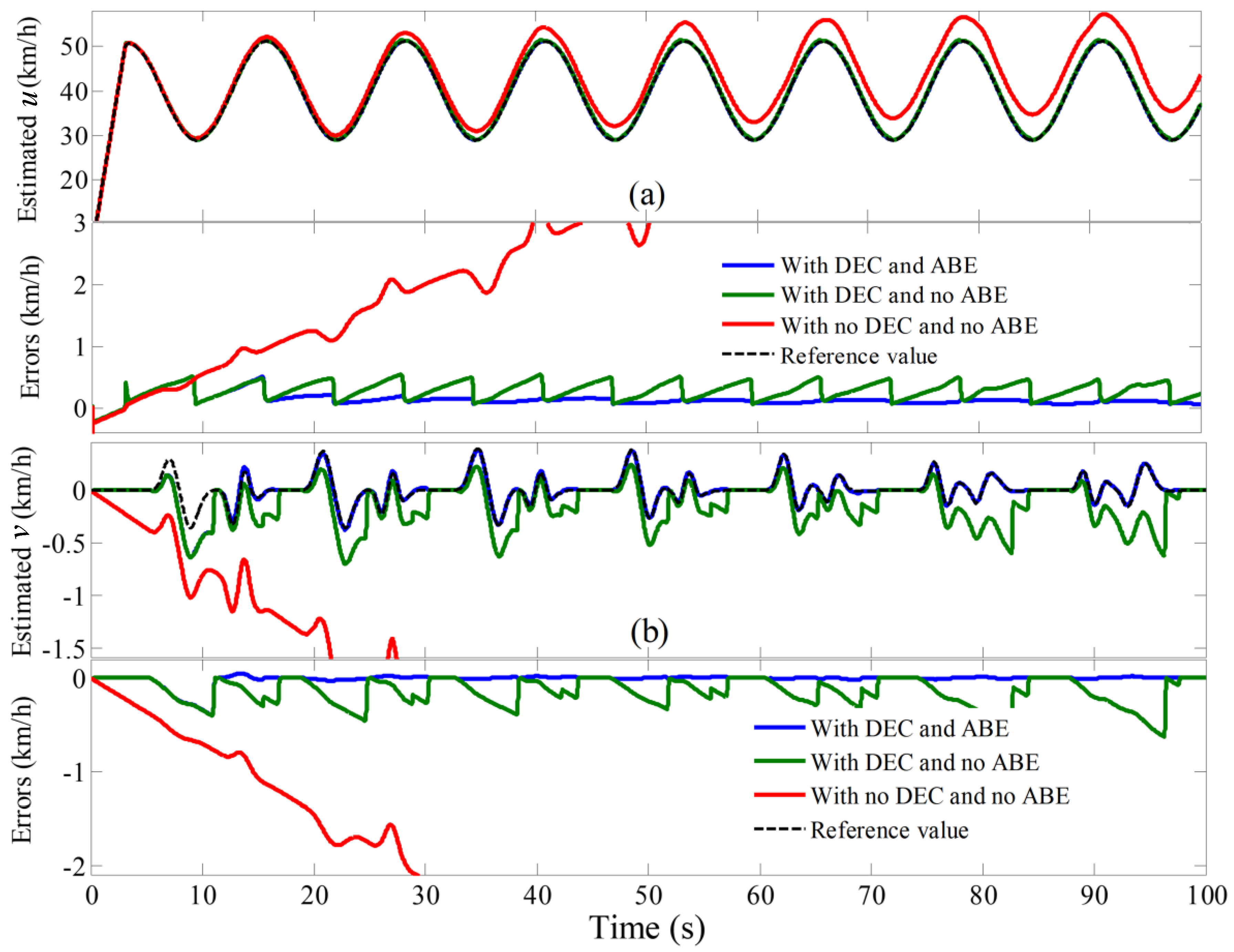
Figure 10a,b show the estimation results of the longitudinal and lateral velocities respectively. Estimation results under three kinds of algorithms, including the algorithms with both DEC and ABE, with DEC and no ABE, and without both DEC and ABE, are compared with each other. It is shown that, without DEC and ABE, the estimated velocities diverge with the accumulative integral error; with DEC and no ABE, the velocities are accurately estimated when they are strongly corrected by the DEC at appropriate time instants for intervals, however, due to the existence of the acceleration biases, accumulative integral errors still exist between the adjacent strong DEC points or intervals. Most significantly, with both the DEC and the ABE, the estimation errors of the velocities are effectively restricted within a small range on both long and short timescales.
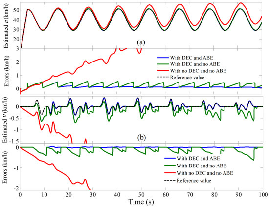
Figure 10.
The estimated velocities during the consecutive DLC test: (a) longitudinal velocity; (b) lateral velocity.
4.3. Ring-Road Test with Varying Curvature and Speed
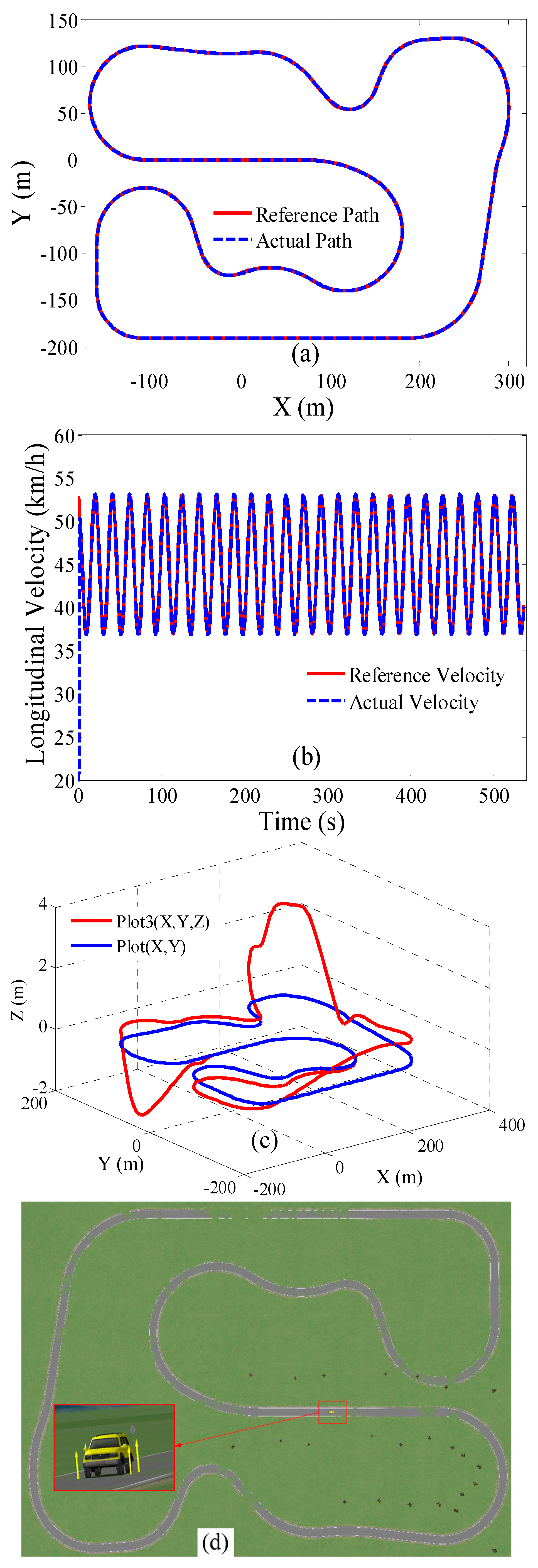
To further verify the performance of the estimation algorithm in a more general way, a custom-defined ring-road test with varying speed is designed. The projection of the ring-road in the X-Y plane is depicted in Figure 11a. The mileage of the ring-road is 2.23 km and the road adhesion coefficient is set as 0.8. In addition, a wide range of curvature is distributed in different sections of the road. Meanwhile, to retain generality, a varying road elevation is added to the road to represent the varying road gradient. The 3D profile and the airview map of the ring-road are shown in Figure 11c,d respectively. The initial speed is set as 5 km/h, and a cosine-wave varying speed with the frequency of 0.3 rad/s, the amplitude of 10 km/h and the average speed of 45 km/h is designed as the target speed, as shown in Figure 11b. The varying range of the speed is deliberately designed for the vehicle to drive through the whole ring-road safely and stably. The acceleration biases are set the same as in Part B. The vehicle drives through the ring-road three times circularly, allowing enough time and distance for the ABE algorithm to converge.

Figure 11.
The tracking results of the ring-road test: (a) path tracking projection in X-Y plane; (b) speed following result; (c) 3D profile of the ring-road; (d) airview map of the ring-road.
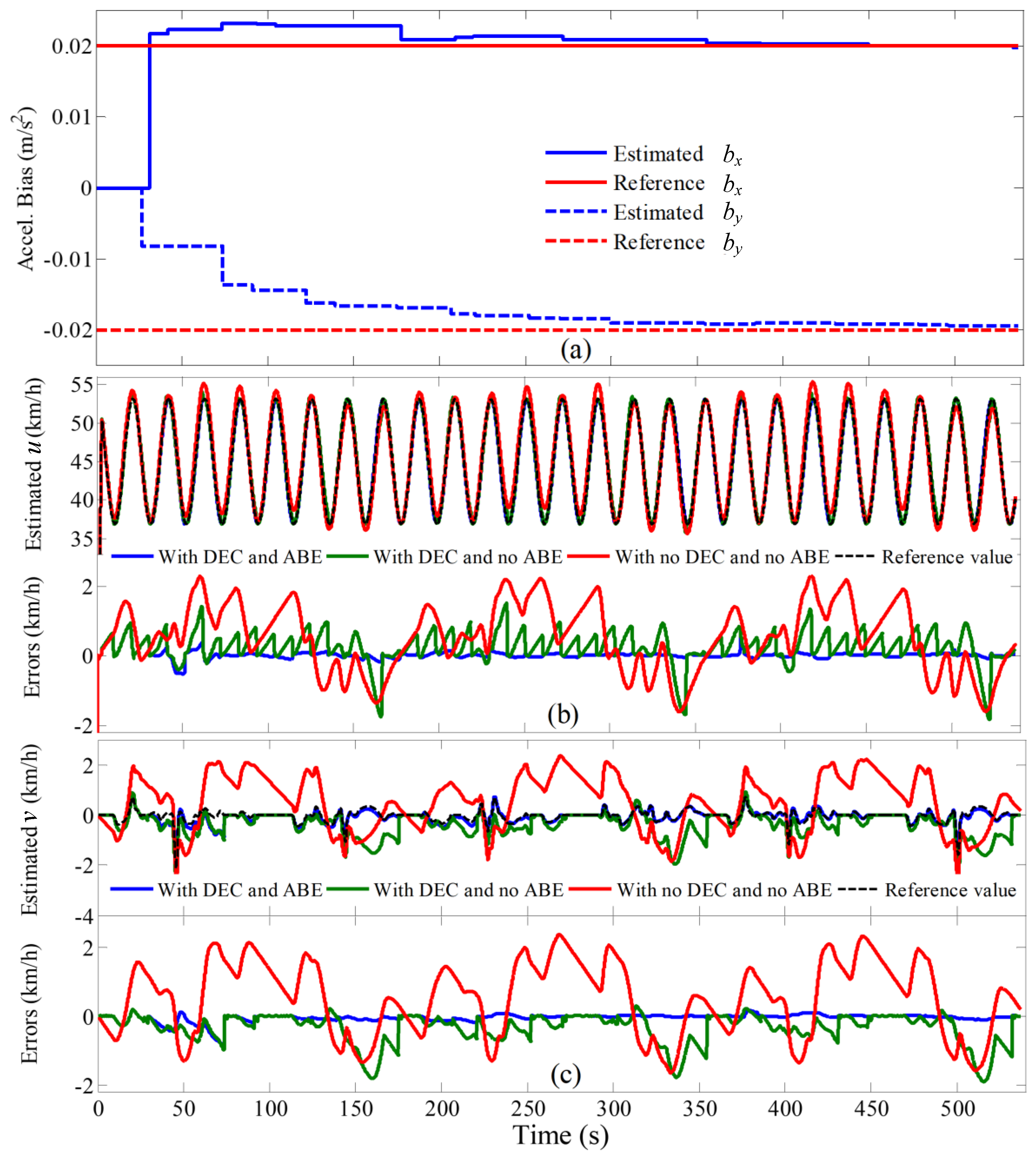
The estimated accelerations biases and the velocities are shown in Figure 12. In Figure 12a, the estimated accelerations biases are eventually identified after a self-learning process of about two cycles, and it takes some time for the RLS-F algorithm to converge. The results of the estimated velocities are similar to the results in Part B, without DEC and ABE, great estimation errors are caused by the accumulative integral error, however, the results do not diverge as in Part B, which is caused by the coupling relation between the velocities and the yaw rate in the consecutive circular driving operation; with DEC and no ABE, the estimated velocities are effectively and occasionally corrected by the driving experiences, however, between the adjacent DEC points, the accumulative integral errors still exist due to the acceleration biases. As the result of both DEC and ABE, both at the strong DEC points and in the ordinary integral intervals, the estimation errors of the velocities are restrained at a very low level relative to the other results. In summary, during the ring-road test, the proposed algorithm generates an accurate and reliable estimation of the longitudinal and lateral velocities with the assistance of DEC on long timescale and the ABE on short timescale.
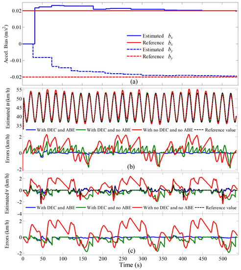
Figure 12.
The estimation results during the ring-road test: (a) acceleration biases (b) longitudinal velocity; (c) lateral velocity.
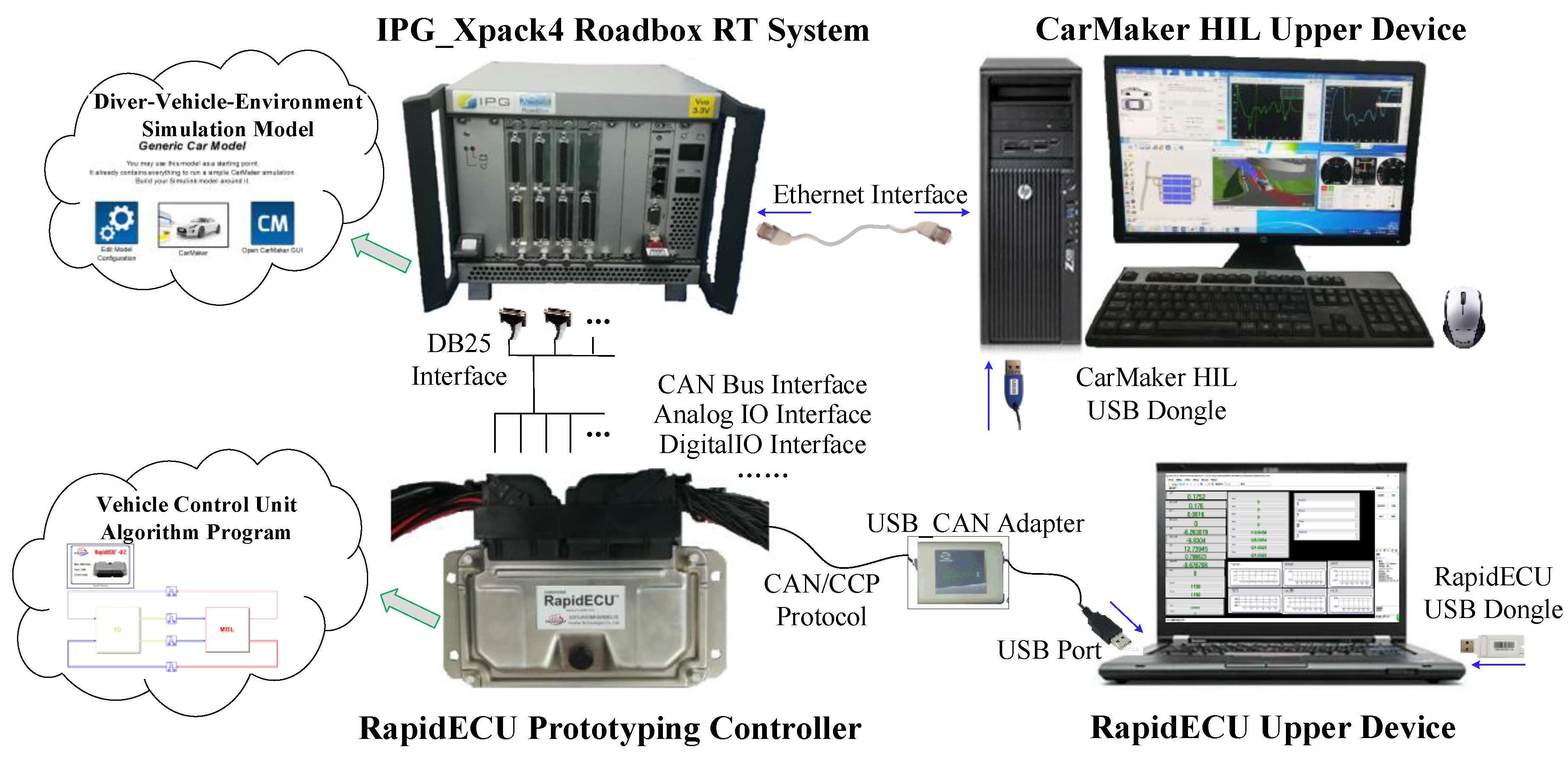
5. Controller-in-the-Loop Test Analysis
To future verify the performance of the proposed estimation algorithm when operating in the VCU under real-time condition, we established the HIL platform for the controller-in-the-loop (CIL) test by combing the rapid prototyping controller, the IPG-RoadBox real-time system, the IPG-CarMaker software(Version 6.0.3, IPG Automotive GmbH, Karlsruhe, Germany) environment and the Simulink RTW Coder tools, as shown in Figure 13. Currently, lots of research work have been done about establishing the co-simulation platform considering the traffic flow for automated driving testing purposes [35]. In our HIL co-simulation platform, the IPG-Xpack4 RoadBox severs as the real-time simulation hardware for driver-vehicle-environment model; The CarMaker HIL upper device severs as The RapidECU Prototyping Controller is equipped with an automotive-level micro processing chip (MPC5644), and it serves as the data collection and calculation platform for the proposed estimation algorithm; The RapidECU upper device provides the user interface for the coding, complying, monitoring and calibrating of the proposed estimation algorithm. The measured signals of the Multi-axis IMU and the wheel speeds are transmitted from the IPG-Xpack4 RoadBox to the RapidECU Prototyping Controller via CAN bus with a period of 20 ms, and the steering wheel angle is transmitted via the analog-digital IO interface with the sampling rate of 5 ms.

Figure 13.
The HIL platform for the CIL test.
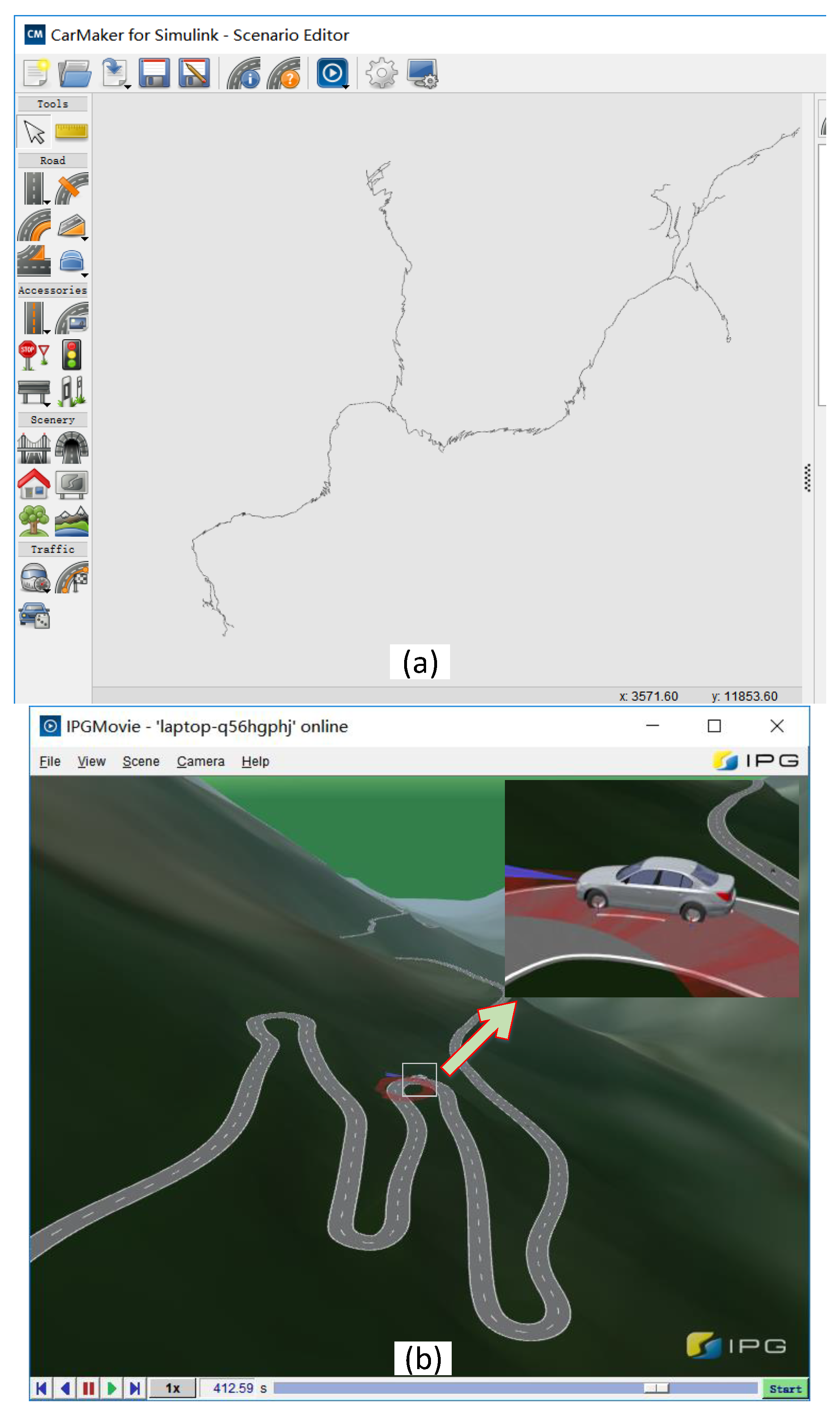
An example mountain-road driving environment provided by the IPG-CarMaker’s demo library is chosen as the CIL test condition. The driver model maintains the global cruising speed of the 60 km/h when driving straightly and adjusts the driving speed according to the local road curvature when steering for safety. Figure 14a,b show the global 2D aerial view and the local 3D road condition of the mountain road respectively. The road data is constructed according to the high-precision satellite map of a certain real place. The simulation time is 500 s, and the total simulated driving mileage is 7.3 km. The whole driving process covers a wide range of driving maneuvers, such as straight driving, uphill and downhill driving, rapid turning with large and small curvatures, rapid acceleration and deceleration, etc. The performance of the estimation algorithm under such driving condition is more representative and persuasive. The longitudinal and lateral measured acceleration biases are set as 0.02 m/s2 and −0.015 m/s2, respectively.

Figure 14.
The mountain-road driving condition: (a) the global 2D aerial view; (b) the local 3D road scene diagram.
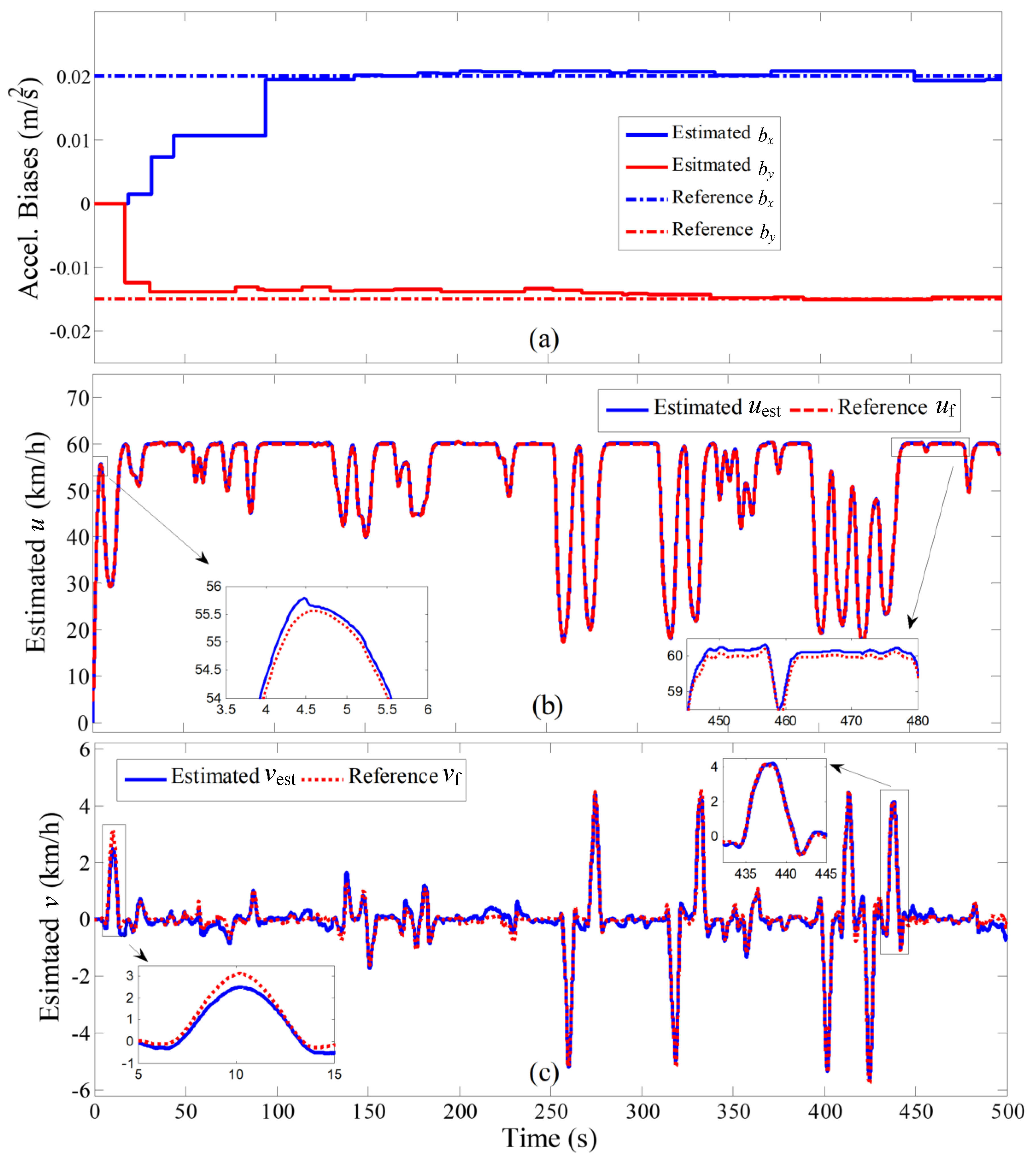
Figure 15 shows the identified acceleration biases and the estimated longitudinal and lateral velocities in the complex mountain-road driving condition. Figure 15a shows that within the first 100 s, the estimated longitudinal and lateral acceleration biases are updated 4 times and 3 times respectively, and the preset reference values are eventually identified. Figure 15b shows that the vehicle maintains a global cruising speed of 60 km/h, and the driver reduces the speed when turning at a different road curve if necessary, and the minimum speed reached is below 20 km/h. When the biases of the accelerations are not effectively identified in the beginning stage, a considerable integral error exists in the estimated longitudinal velocity, but at the critical point between accelerating and decelerating, the estimated longitudinal velocity is effectively corrected based on the average wheel speed. Figure 15c shows that the estimated lateral velocity is also affected by the unidentified acceleration biases in the initial stage. With the accuracy of the identified acceleration biases are improved after 100 s, the accuracy of the estimated lateral velocity is synchronously improved. In addition, when the lateral velocity is small, the relative error of the estimation results is greater because of the low signal-noise ratio of the IMU signals. However, when the empirical straight driving condition (Wy = 0) holds, the estimated lateral velocity is corrected to zero, which eliminates the accumulation error caused by kinematic integral. To sum up, the CIL test shows that within the 7.3 km driving mileage, the measuring acceleration biases are effectively identified; the relative estimation error of the longitudinal velocity is constrained within 2%; and the estimation error of the lateral velocity is less than 0.5 km/h.
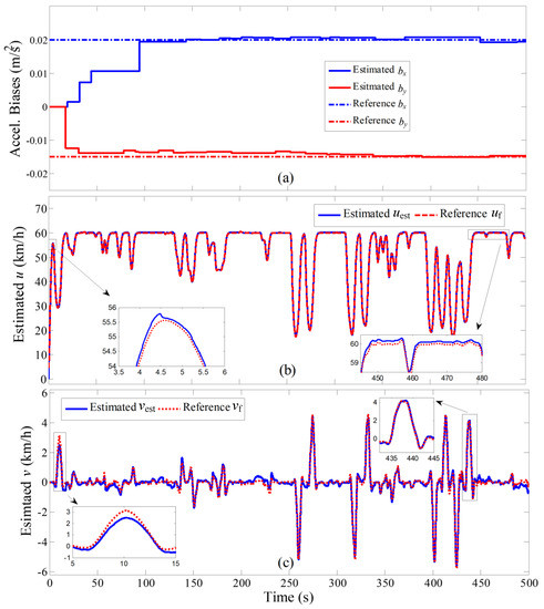
Figure 15.
The estimation results of the mountain-road test: (a) acceleration biases (b) longitudinal velocity; (c) lateral velocity.
6. Conclusions
An estimation method for the longitudinal and lateral vehicle velocities fusing with kinematic integral and empirical correction on multi-timescales is proposed. The algorithm needs only a low-cost multi-axis IMU sensor, wheel speed encoders, a steering wheel angle sensor and the effective rolling radius. The algorithm is practical since it is non-tire-model-based and no other unavailable signals or frequently changeable model parameters are required. Two reliable judgements about the longitudinal and lateral velocities are extracted from the available signals, which performs good empirical correction for the accumulative integral errors of the kinematics equations on long timescale. Furthermore, the biases of the measured accelerations are also estimated recursively by comparing the integral of the measured accelerations with the difference of the estimated velocities between the adjacent strong DEC instants, which corrects integral error of kinematic equations on short timescale. The algorithm provides accurate and reliable vehicle velocities estimation results, which is particularly meaningful for developing the advanced vehicles control systems for electric vehicles and autonomous vehicles.
To verify the performance of the estimation algorithm, a consecutive DLC test and a ring-road test with varying speed are simulated by the CarSim-Simulink co-simulation, and a complex mountain-road test is carried out by the controller-in-the-loop test under CarMaker-RoadBox environment. A four-wheel-independently motor-driven electric vehicle is chosen as the test platform. The results show that with the integration of the DEC on long timescale and the ABE on short timescale, the identified measuring acceleration biases converge to their preset values within finite time, and the relative estimation error of the longitudinal velocity and the absolute estimation error of the lateral velocity are restrained within 2% and 0.5 km/h, respectively.
Author Contributions
H.H. and Y.C. contributed to the conception of the study; J.L. and W.L. developed the estimation algorithm; W.L. and J.L. carried out the simulation and controller-in-the-loop test; F.S. performed the analysis with constructive discussions.
Funding
This work is partly supported by the National Key Research and Development Program of China (2017YFB0103802). And it is also partly supported by the General Program of National Natural Science Foundation of China (51675042).
Conflicts of Interest
The authors declare no conflict of interest.
Abbreviations
| IMU | Inertia Measurement Unit |
| DOF | Degree of Freedom |
| GPS | Global Positioning System |
| DEC | Driving Empirical Correction |
| ABE | Acceleration Bias Estimation |
| VCU | Vehicle Control Unit |
| RLS-F | Recursive Least Square algorithm with forgetting factor |
| DLC | Double Lane Change |
| RTW | Real-Time Workshop |
| HIL | Hardware-in-the-loop |
| CIL | Controller-in-the-loop |
| CG | Center of Gravity |
References
- Hashemi, E.; Pirani, M.; Khajepour, A.; Kasaiezadeh, A. Corner-based estimation of tire forces and vehicle velocities robust to road conditions. Control Eng. Pract. 2017, 61, 28–40. [Google Scholar] [CrossRef]
- Wang, X.M.; He, H.W.; Sun, F.C.; Sun, X.K.; Tang, H.L. Comparative study on different energy management strategies for plug-in hybrid electric vehicles. Energies 2013, 6, 5656–5675. [Google Scholar] [CrossRef]
- Guo, H.Q.; He, H.W.; Sun, F.C. A combined cooperative braking model with a predictive control strategy in an electric vehicle. Energies 2013, 6, 6455–6475. [Google Scholar] [CrossRef]
- He, H.W.; Peng, J.K.; Xiong, R.; Fan, H. An acceleration slip regulation strategy for four-wheel drive electric vehicles based on sliding mode control. Energies 2014, 7, 3748–3763. [Google Scholar] [CrossRef]
- Liu, W.; He, H.W.; Sun, F.C. Vehicle state estimation based on Minimum Model Error criterion combining with Extended Kalman Filter. J. Frankl. Inst. 2016, 353, 834–856. [Google Scholar] [CrossRef]
- Rezaeian, A.; Khajepour, A.; Melek, W.; Chen, S.K.; Moshchuk, N. Simultaneous Vehicle Real-Time Longitudinal and Lateral Velocity Estimation. IEEE Trans. Veh. Technol. 2017, 66, 1950–1962. [Google Scholar] [CrossRef]
- Hac, A.; Nichols, D.; Sygnarowicz, D. Estimation of Vehicle Roll Angle and Side Slip for Crash Sensing; SAE Technical Paper; SAE International: Warrendale, PA, USA, 2010; pp. 1–529. [Google Scholar]
- Kim, H.H.; Ryu, J. Sideslip angle estimation considering short duration longitudinal velocity variation. Int. J. Automot. Technol. 2011, 12, 545–553. [Google Scholar] [CrossRef]
- Klomp, M.; Gao, Y.; Bruzelius, F. Longitudinal velocity and road slope estimation in hybrid electric vehicles employing early detection of excessive wheel slip. Veh. Syst. Dyn. Int. J. Veh. Mech. Mobil. 2014, 52, 172–188. [Google Scholar] [CrossRef]
- Piyabongkarn, D.; Rajamani, R.; Grogg, J.A.; Lew, J.Y. Development and experimental evaluation of a slip angle estimator for vehicle stability control. IEEE Trans. Control Syst. Technol. 2009, 17, 78–88. [Google Scholar] [CrossRef]
- Fukada, Y. Slip-angle estimation for vehicle stability control. Vehicle Syst. Dyn. 1999, 32, 375–388. [Google Scholar] [CrossRef]
- Kim, J.; Lee, H.; Choi, S. A robust road bank angle estimation based on a proportional-integral H∞ filter. Proc. Inst. Mech. Eng. D J. Autom. Eng. 2012, 226, 779–794. [Google Scholar] [CrossRef]
- Ghandour, R.; Victorino, A.; Doumiati, M.; Charara, A. Tire/road friction coefficient estimation applied to road safety. In Proceedings of the 18th Mediterranean Conference on Control and Automation, MED’10, Marrakech, Morocco, 23–25 June 2010; pp. 1485–1490. [Google Scholar]
- Canudas-de-Wit, C.; Tsiotras, P. Dynamic tire friction models for vehicle traction control. In Proceedings of the 38th Conference on Decision & Control, Phoenix, AZ, USA, 7–10 December 1999; pp. 3746–3751. [Google Scholar]
- Canudas-de-Wit, C.; Tsiotras, P.; Velenis, E.; Basset, M.; Gissinger, G. Dynamic friction models for road/tire longitudinal interaction. Vehicle Syst. Dyn. 2003, 39, 189–226. [Google Scholar] [CrossRef]
- Pacejka, H.B.; Bakker, E. Magic formula tyre model. Vehicle Syst. Dyn. 1993, 21, 1–18. [Google Scholar] [CrossRef]
- Guo, K.H. UniTire: United Tire Model. J. Mech. Eng. 2016, 52, 90–99. [Google Scholar] [CrossRef]
- Tang, Y.G.; Wu, Y.X.; Wu, M.P.; Wu, W.Q.; Hu, X.P.; Shen, L.C. INS/GPS Integration: Global Observability analysis. IEEE Trans. Veh. Technol. 2009, 58, 1129–1142. [Google Scholar] [CrossRef]
- Guan, X.; Yan, D.; Gao, Z.H. Vehicle movement state test system based on INS/RTKDGPS. J. Jilin Univ. 2006, 36, 14–19. [Google Scholar]
- Li, X.; Chan, C.Y.; Wang, Y. A reliable fusion methodology for simultaneous estimation of vehicle sideslip and yaw angles. IEEE Trans. Veh. Technol. 2016, 65, 4440–4458. [Google Scholar] [CrossRef]
- Farrell, J.A.; Tan, H.S.; Yang, Y. Carrier phase gps-aided ins-based vehicle lateral control. J. Dyn. Syst. Meas. Control 2003, 125, 339–353. [Google Scholar] [CrossRef]
- Bevly, M. Global positioning system (gps): A low-cost velocity sensor for correcting inertial sensor errors on ground vehicles. J. Dyn. Syst. Meas. Control 2004, 126, 255–264. [Google Scholar] [CrossRef]
- Bevly, M.; Ryu, J.; Gerde, J.C. Integrating ins sensors with gps measurements for continuous estimation of vehicle sideslip, roll, and tire cornering stiffness. IEEE Trans. Intell. Transp. Syst. 2006, 7, 483–493. [Google Scholar] [CrossRef]
- Yoon, J.H.; Peng, H. A cost-effective sideslip estimation method using velocity measurements from two gps receivers. IEEE Trans. Veh. Technol. 2014, 63, 2589–2599. [Google Scholar] [CrossRef]
- Ryu, J.; Gerdes, J.C. Integrating inertial sensors with global positioning system (gps) for vehicle dynamics control. J. Dyn. Syst. Meas. Control 2004, 126, 243–254. [Google Scholar] [CrossRef]
- Villagra, J.; d’Andréa-Novel, B.; Fliess, M.; Mounier, H. Estimation of longitudinal and lateral vehicle velocities: An algebraic approach. In Proceedings of the 2008 American Control Conference, Seattle, WA, USA, 11–13 June 2008; pp. 3941–3946. [Google Scholar]
- Imsland, L.; Grip, H.F.; Johansen, T.A.; Fossen, T.I.; Kalkkuhl, J.C.; Suissa, A. Nonlinear Observer for Vehicle Velocity with Friction and Road Bank Angle Adaptation–Validation and Comparison with an Extended Kalman Filter; SAE Technical Paper; SAE International: Warrendale, PA, USA, 2007. [Google Scholar]
- Imsland, L.; Johansen, T.A.; Fossen, T.I.; Grip, H.F.; Kalkkuhl, J.C.; Suissa, A. Vehicle velocity estimation using nonlinear observers. Automatica 2006, 42, 2091–2103. [Google Scholar] [CrossRef]
- Naets, F.; Aalst, S.V.; Boulkroune, B.; Ghouti, N.E.; Desmet, W. Design and experimental validation of a stable two-stage estimator for automotive sideslip angle and tire parameters. IEEE Trans. Veh. Technol. 2017, 66, 9727–9742. [Google Scholar] [CrossRef]
- Nam, K.H.; Fujimoto, H.; Hori, Y. Lateral stability control of In-wheel-motor-driven electric vehicles based on sideslip angle estimation using lateral tire force sensors. IEEE Trans. Veh. Technol. 2012, 61, 1972–1985. [Google Scholar]
- Tanelli, M.; Savaresi, S.; Cantoni, C. Longitudinal vehicle speed estimation for traction and braking control systems. In Proceedings of the IEEE International Conference on Control Applications, Munich, Germany, 4–6 October 2006; pp. 2790–2795. [Google Scholar]
- Song, C.K.; Hedrick, J.K. Vehicle Speed Estimation Using Accelerometer and Wheel Speed Measurements; SAE Technical Paper 724; SAE International: Warrendale, PA, USA, 2002. [Google Scholar]
- Jiang, F.J.; Gao, Z.Q. An adaptive nonlinear filter approach to the vehicle velocity estimation for ABS. In Proceedings of the IEEE International Conference on Control Applications, Anchorage, AK, USA, 27 September 2000; Volume 1, pp. 490–495. [Google Scholar]
- Mechanical Simulation Corporation. Carsim 8.0 User Manual. 2009. Available online: http://www.carsim.com/products/carsim/index.php (accessed on 4 January 2019).
- Hallerbach, S.; Xia, Y.; Eberle, U.; Koester, F. Simulation-Based Identification of Critical Scenarios for Cooperative and Automated Vehicles; SAE Technical Paper; SAE International: Warrendale, PA, USA, 2018; Volume 1, pp. 93–106. [Google Scholar]


© 2019 by the authors. Licensee MDPI, Basel, Switzerland. This article is an open access article distributed under the terms and conditions of the Creative Commons Attribution (CC BY) license (http://creativecommons.org/licenses/by/4.0/).