Effect of Prediction Error of Machine Learning Schemes on Photovoltaic Power Trading Based on Energy Storage Systems

Abstract

Photovoltaic (PV) output power inherently exhibits an intermittent property depending on the variation of weather conditions. Since PV power producers may be charged to large penalties in forthcoming energy markets due to the uncertainty of PV power generation, they need a more accurate PV power prediction scheme in energy market operation. In this paper, we characterize the effect of PV power prediction errors on energy storage system (ESS)-based PV power trading in energy markets. First, we analyze the prediction accuracy of two machine learning (ML) schemes for the PV output power and estimate their error distributions. We propose an efficient ESS management scheme for charging and discharging operation of ESS in order to reduce the deviations between the day-ahead (DA) and real-time (RT) dispatch in energy markets. In addition, we estimate the capacity of ESSs, which can absorb the prediction errors and then compare the PV power producer’s profit according to ML-based prediction schemes with/without ESS. In case of ML-based prediction schemes with ESS, the ANN and SVM schemes yield a decrease in the deviation penalty by up to 87% and 74%, respectively, compared with the profit of those schemes without ESS.

1. Introduction

In recent years, the world has faced a urgent climate change problem and a depletion problem of fossil fuels. The portion of renewable energy sources (RESs) has gradually increased instead of fossil fuel based generators in many countries. We expect that worldwide penetration of solar power rapidly increase until 2030 since it is manageable to build, operate, and maintain PV systems [1]. Utility-scale photovoltaic (PV) plants have been rapidly installed in many countries. For example, China, Germany, and the USA have tens of utility-scale PV farms. In addition, China, Japan and European countries have operated a feed-in tariff (FIT) policy to increase investment in PV industry, while the USA and South Korea adopted a renewable portfolio standard (RPS) in order to spread PV systems [2].

However, PV output power generally exhibits an ‘intermittent’ output characteristic depending on weather conditions [3]. Due to the poor predictability, PV systems may experience a power imbalance during those operation. Therefore, it is difficult for MW-scale PV power producers to participate in energy markets due to the prediction errors. Furthermore, this intermittent property may decrease the economical profit for utility-scale PV power producers since higher capacity of energy storage systems (ESSs) is required to absorb the prediction errors of PV power generation and avoid the variability of utility.

Integration of RES output power in the power system would highly depend on accurate forecasts [4,5]. Therefore, a number of studies on the prediction of solar irradiance or PV output power have been found in literature. The persistence scheme may be effective only for its use in short-term forecast (e.g., intra-hour) applications [6]. Cloud motion vector (CMV) by total sky imagers [7] and satellite images [8] were utilized to analyze cloud movement and predict short-term irradiance at the ground level. For longer time horizons (hours to days), numerical weather prediction (NWP) schemes have been applied [9,10]. A number of time series prediction schemes such as autoregressive moving average (ARMA) [11], autoregressive integrated moving average (ARIMA) [12], and autoregressive moving average with exogenous inputs (ARMAX) [13] have also been used to design the prediction model based on stochastic characteristics of solar irradiance. In addition, a number of prediction studies have developed nonlinear solar or PV output power prediction schemes based on machine learning (ML). In specific, artificial neural networks (ANN) [14], support vector machine (SVM) [15,16], and hybrid schemes [17] have been utilized in prediction models.

The Federal Energy Regulatory Commission (FREC) issued the Order 764, which aims to remove a barrier for the integration of renewable energy resources into the power grid [18]. In the existing energy market, the FERC noted that the suppliers of renewable energy resources should pay for imbalance penalties for any difference between their settled energy and actual delivery in that hour. In addition, the suppliers of renewable energy resources need to provide bids in RT markets, based on forecasts and then follow dispatch instructions in the current Independent System Operator (ISO)/Regional Transmission Organization (RTO) markets [19]. New York (NYISO), PJM Interconnection (PJM), Electric Reliability Council of Texas (ERCOT), and California ISO (CAISO) have the market policy of the imbalance settlements and deviation penalties. If renewable generation is a capacity resource, it must bid in DA market and RT market. Also, a deviation penalty applies. However, the previous PV power prediction studies did not consider the energy market for PV power trading. Few studies dealt with energy markets, which are regulation markets [20,21] and locational marginal price (LMP) markets [4,22] for wind power trading.

ESSs play an important role in integrating RES into power grid. However, there are only few studies considering the contributions of the renewable prediction schemes based on the economic analysis such as an assessment of the profit for the PV power producers. The power capacity of ESSs was calculated to compensate the wind power generation [23]. However, the operational environment of the ESS is different for absorbing the deviation due to the prediction errors between the wind and PV systems. For example, ESSs for the PV system can be operated at night and day time from the power grid in order to prevent an unnecessary increase in the energy capacity. The capacity of ESSs was calculated to reduce the power fluctuation of PV output power in [24]. However, the authors did not consider the uncertainty of the prediction schemes. As a result, the previous studies on the ESS operation strategy mainly focused on cost minimization of a given system under a Time-of-Use (ToU) pricing or real-time pricing [25,26]. It is evident that the prior studies often neglected the uncertainty of forecasting PV output power. Therefore, it should be considered to provide the accurate operation for various operational conditions. In this paper, by using the prediction scheme, we propose an efficient ESS management scheme in order to estimate the accurate deviation penalties in energy markets.

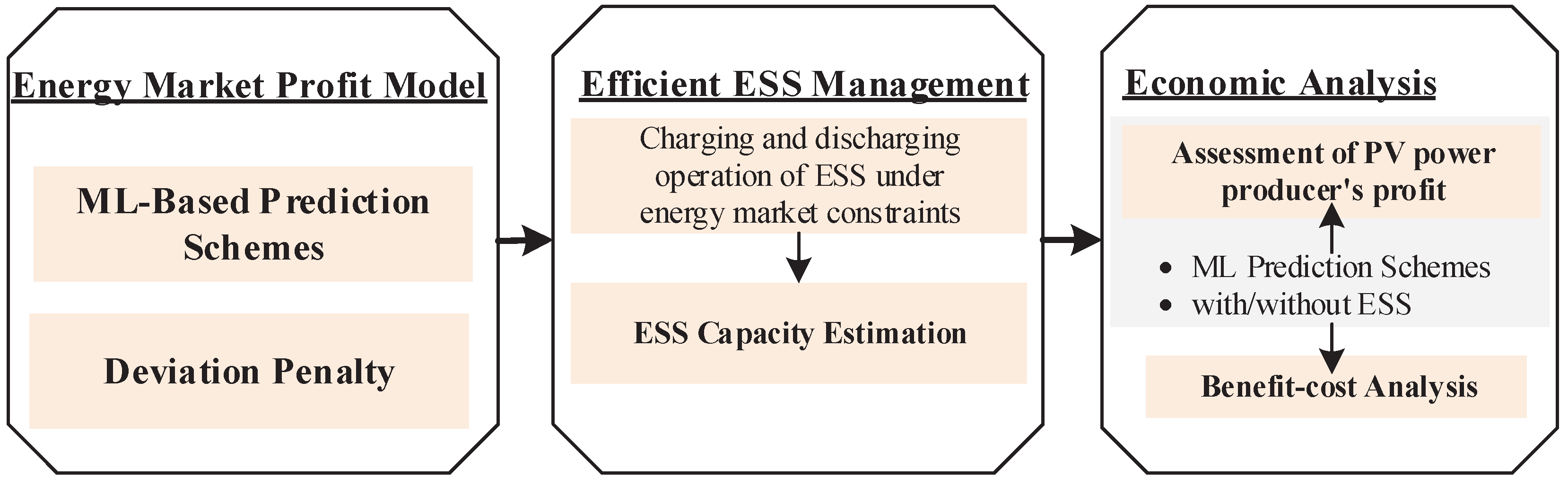
In this paper, we estimate the effect of the prediction errors on energy storage system (ESS)-based PV power trading as shown in Figure 1. First, we evaluate the performance of PV power prediction models with the ANN and SVM schemes, and their prediction errors are fitted by a t location-scale distribution in order to describe a characteristic of heavy tails. And then, we characterize the ESS role in forthcoming energy markets and propose an efficient ESS management scheme for charging and discharging operation of ESS in order to reduce the deviation penalties from differences between day-ahead (DA) schedule and real-time (RT) supply in energy markets. As a case study, we estimate the capacity of ESSs from different energy market constraints in terms of a tolerance limit and a penalty factor. We calculate the PV power producer’s profit considering the deviation penalties in case of ML-based prediction schemes with/without ESS in order to quantitatively estimate the effect of ESS for different prediction accuracies of two ML-based prediction schemes. As a result, we analyze the benefit from the accurate prediction scheme with ESS management as a case study on the participation of a utility-scale PV farm at a locational marginal price (LMP) market in the United States. Furthermore, we study the economic analysis of ESS installation for using both the ANN and SVM schemes through the benefit cost analysis (BCA).

Some studies have investigated the economic analysis of PV systems based on the installation cost analysis [26]. And, few studies have considered the uncertainty of the renewable power prediction for renewable power trading. A persistence prediction scheme was utilized in order to estimate the profit for wind energy trading [22]. But, they did not consider ML-based prediction schemes. In addition, the distributions of PV prediction errors is slightly different from that of wind power prediction errors. Therefore, it is valuable to apply the accurate prediction scheme based on ML in PV power trading. Also, more quantitative analysis is required for analyzing the effect of the prediction accuracy for PV power trading in detail. The contributions of this paper can be summarized as follows: (1) We estimate the accuracy of two ML-based prediction schemes and characterize their error distributions in order to quantitatively estimate the effect of the prediction accuracy for PV power trading; (2) The capacity of ESSs, which can reduce cost associated with PV prediction errors for PV power trading, is estimated from different market parameters; (3) In case of ML-based prediction schemes with/without ESS, the benefit from the accurate prediction scheme with ESS management is analyzed as a case study; (4) The economic analysis of ESS installation for two ML-based prediction schemes is done through the BCA.

The rest of this paper is organized as follows. We briefly introduce two ML-based prediction schemes for PV output power in Section 2. In Section 3, we estimate the prediction accuracy of two ML-based prediction schemes and their error distributions for PV output power prediction. In Section 4, we characterize the ESS role and describe the participation of PV producers in forthcoming energy markets. And then, we determine the efficient ESS management, which consists of the operation and sizing of ESS for PV power trading in forthcoming energy markets. In Section 5, we analyze the benefits from the accurate prediction scheme with ESS management as a case study. Finally, we give conclusive remarks in Section 6.

2. Background

2.1. Artificial Neural Networks

Artificial neural networks (ANNs), which resemble a human brain, have been extensively applied to uncertain problems. They have been widely used as an alternative method in engineering analysis and prediction such as computer vision and speech recognition [27]. ANNs do not require any detailed information from the system. Instead, ANNs learn the relationship between the input parameters. The controlled and uncontrolled variables by characterizing the collected data and may depend on a large number of input parameters [28].

ANNs are typically specified using the architecture, activity rules, and learning rules [29]. Figure 2 shows a structure of a feed-forward ANN architecture. The ANN network has an input layer, hidden layers and an output layer.

The j-th node in the hidden layer, $z_j$ is expressed as

$$\begin{array}{c}\hfill z_j=g(\sum _{k=1}^K{w}_{k,j}{x}_k+b),\end{array}$$

(1)

where $g(a)$ is an activation function, such as unit step, sigmoid, and hyperbolic tangent functions. $x_k$ is the k-th input value and $w_{k,j}$ is the weight between the k-th input node and the j-th hidden node. b is a bias value. Furthermore, The value of the output node, y is calculated as

$$\begin{array}{c}\hfill y=\sum _{j=1}^J{v}_j{z}_j+c=\sum _{j=1}^J{v}_{j}g(\sum _{k=1}^K{w}_{k,j}{x}_k+b)+c,\end{array}$$

(2)

where $v_j$ is the weight between the j-th hidden node and the output node. c is another bias value.

We here use an ANN to model the complex relationship between various meteorological elements and PV output power in order to improve the prediction performance. The ANN model has two-layered feed-forward network with sigmoid functions, which is defined as $g(a)=1/(1+e^{-a})$ and linear output neurons. We use 20 neurons in the hidden layer and train the network with the Levenberg-Marquardt back propagation algorithm [30]. We finally obtain the predicted value ${\widehat{y}}_i=f({\mathit{x}}_i)$ where ${\widehat{y}}_i$ is the i-th predicted value and ${\mathit{x}}_i$ is the i-th input column vector.

2.2. Support Vector Machine

Support vector machine (SVM) is one of high-performance machine learning (ML) schemes, which was proposed by Cortes and Vapnik [31]. SVM is designed to minimize the error and maximize the separation margin among multiple classes [32]. In particular, SVM can be used to train solar PV output power and predict their output in advance. It has been proved that a better learning capability and smaller prediction errors can be achieved than other methods by using a hyperplane trick [16].

We define a observation sample set of N input and output data as $D=\{({\mathit{x}}_1,y_1),({\mathit{x}}_2,y_2),\dots ,({\mathit{x}}_N,y_N)\}\in R^K\times R.$ A regression function is expressed as

$$\begin{array}{c}\hfill F=\{f\mid f({\mathit{x}}_i)={\mathit{w}}^{\mathrm{T}}·{\mathit{x}}_i+b,\mathit{w}\in R^K\},\end{array}$$

(3)

where $\mathit{w}$ is the unit normal vector, ${\mathit{x}}_i$ is the input vector, and b is the distance from the origin to the hyperplane.

The main idea of typical SVM is to map the input vector ${\mathit{x}}_i$ into higher-order feature spaces by using a non-linear kernel function, and performs linear regression in the higher-order feature space as follows [33].

$$\begin{array}{c}\hfill \min \left(\frac{1}{2}{∥\mathit{w}∥}^2+C\sum _{i=1}^M{\zeta }_i\right)\end{array}$$

(4)

subject to

$$\begin{array}{c}\hfill y_i({\mathit{w}}^{\mathrm{T}}·\phi ({\mathit{x}}_i)+b)\ge 1-{\zeta }_i,{\zeta }_i\ge 0\end{array}$$

(5)

where ${\zeta }_i$ and M represent a slack variable and the number data for training stage, respectively. C is a positive constant value for regularization. The mapping function of $\phi ({\mathit{x}}_i)$ can be replaced by some special kernels $K({\mathit{x}}_i,{\mathit{x}}_j)$. We utilize a radial basis function (RBF) as a kernel function in this study. The RBF kernel is represented as follows:

$$\begin{array}{c}\hfill K({\mathit{x}}_i,{\mathit{x}}_j)=\exp \left(-\frac{{∥{\mathit{x}}_i-{\mathit{x}}_j∥}^2}{{\delta }^2}\right),\end{array}$$

(6)

where $\delta$ represents the dilation parameter determining the width of the kernal. In addition, we utilize the LibSVM software [34] in order to develop the SVM scheme.

3. PV Output Power Prediction

3.1. Data for PV Output Power Prediction

We have collected actual meteorological data for 26 months (January 2012 to April 2014) from the Korea Meteorological Administration (KMA) in Daejeon (36.37 ${}^{\circ }\mathrm{N}$, 127.37 ${}^{\circ }\mathrm{E}$) to develop the prediction models [35]. The sampling interval is one hour. The sunshine duration is set from 7:00 A.M. to 6:00 P.M.

Table 1. Meteorological parameters and value range.

Meteorological Parameters	Value Range
Irradiance $[{\mathrm{W}/\mathrm{m}}^2]$	0–1083
Sunshine Duration	7:00 A.M. to 6:00 P.M.
Cloud Cover	0–10
Sunshine [hour]	0–1
Humidity [%]	10–100
Precipitation [mm/h]	0–40
Air Temperature [${}^{\circ }\mathrm{C}$]	−16–37
Wind Speed [m/s]	0–11

summarizes the various meteorological parameters. Specifically, cloud cover refers to the fraction of the sky obscured by clouds at a particular location with a range of 0 to 10. When 70% of the area was occupied by clouds the cloud cover value becomes 7. Also, there are 10 types of clouds in the measured data from the weather station in Daejeon. Those data is observed by the weather satellite, Chollian, which is independent weather observation system from space.

The solar irradiance at the i-th time sequence is set to a single output, and the other parameters at the i-th time sequence are configured as an input vector. We utilize 80% and 20% of the entire data for the training process and the test step, respectively. In this paper, we utilized the measured meteorological data from the weather station instead of the forecasted meteorological data in both stages due to the difficulty of collecting the forecasted meteorological data.

3.2. Prediction Results for PV Output Power

We convert the irradiance into PV output power based on the prediction data in [15]. In this paper, we assume that the PV output power is linearly proportional to the irradiance without considering the module temperature. We do not consider some conversion errors in this paper. Therefore, the PV output power of the i-th time, $P_i$ is estimated as $P_i=C_{\mathrm{PV}}\times \frac{y_i}{1000}$ without consideration of temperature, where $C_{\mathrm{int}}$ is a given PV system capacity.

Figure 3 shows the PV prediction results of the ANN and SVM schemes and the actual PV power values. The prediction horizon is one-hour ahead in this results. At least one-hour ahead prediction is required because PV power producers can submit re-bids at one-hour ahead of the operating hour in the PV power trading [19]. Both schemes show lower prediction accuracy for cloudy days, compared with sunny days. In addition, we can observe that SVM scheme has lower errors than the ANN scheme in both sunny and cloudy days. The weather based data clustering enhances the accuracy of the PV power prediction for severe intermittency [15]. But, we did not consider the weather classification in this paper.

In order to evaluate the prediction accuracy, Root Mean Square Error (RMSE), ${\mathrm{R}}^2$ (coefficient of determination) are used, i.e.,

$$\begin{array}{c}\hfill \mathrm{RMSE}=\sqrt{\frac{{\sum }_{i=M+1}^N{(y_i-f({\mathit{x}}_i))}^2}{N-M}},\end{array}$$

(7)

$$\begin{array}{c}\hfill {\mathrm{R}}^2=1-\frac{{\sum }_{i=M+1}^N{(y_i-f({\mathit{x}}_i))}^2}{{\sum }_{i=M+1}^N{(y_i-\overline{y})}^2},\end{array}$$

(8)

where $y_i$ is the measured value at each time sequence i and $f({\mathit{x}}_i)$ is the prediction result at each time sequence i. $(N-M)$ denotes the total number of data for the test.

The numerical result of ${\mathrm{R}}^2$ of SVM prediction scheme are 58.72$[{\mathrm{W}/\mathrm{m}}^2]$, $0.9562$, while that of the ANN scheme are 71.41$[{\mathrm{W}/\mathrm{m}}^2]$, $0.9264$, respectively.

3.3. Estimation of Prediction Error Distribution

The t location-scale distribution has been utilized for fitting data distributions with heavier tails, compared with the normal distribution [36]. The probability density function (PDF) of the t location-scale distribution is expressed as

$$\begin{array}{c}\hfill h(\epsilon |\nu ,\mu ,\sigma )=\frac{\mathsf{\Gamma }\left(\frac{\nu +1}{2}\right)}{\mathsf{\Gamma }\left(\frac{\mu }{2}\right)\sqrt{\nu \pi }\sigma }{\left\{1+\frac{1}{\nu }{\left(\frac{\epsilon -\mu }{\sigma }\right)}^2\right\}}^{-\left(\frac{\nu +1}{2}\right)},\end{array}$$

(9)

where $\mathsf{\Gamma }(·)$, $\mu$, $\sigma$, and $\nu$ represent the gamma function, the location parameter, the scale parameter, and the shape parameter, respectively. The distribution is parameterized with mean and variance of $\mu$ and ${\sigma }^2\nu /(\nu -2)$, respectively. In this paper, $\epsilon$ represents the prediction error expressed as a ratio of the installed PV capacity in [p.u.].

In order to measure the tail weight and the peakedness of the probability distribution the kurtosis $\kappa$ value can be utilized [37]. In particular, the kurtosis with zero mean random variable $\epsilon$ is defined as follows:

$$\begin{array}{c}\hfill \kappa =\frac{\mathbb{E}[{\epsilon }^4]}{s^4},\end{array}$$

(10)

where $\mathbb{E}$ and s represents the expectation operator and the standard deviation.

In general, a higher kurtosis distribution has heavier tails, while a lower kurtosis distribution has thinner tails. If $\kappa$ value is greater than 3, the distribution is expressed as leptokurtic or fat-tailed with tails that approach zero more slowly than the normal distribution (c.f. the kurtosis of the normal distribution is 3).

In order to obtain the PDF of the prediction errors, we first calculate $\kappa$ values of three prediction schemes. As a result, $\kappa$ values of the ANN and SVM schemes are obtained as $4.59$ and $6.11$, respectively. We observe that the PV output prediction errors of each prediction scheme are not precisely fitted with a normal distribution because those $\kappa$ values are in the rage between $3.9$ and $7.5$, which is heavier-tailed or leptokurtic. Hence, we approximately model the PV power prediction errors of ML-based prediction schemes with a t location-scale distribution, which can well fit heavier tail distributions [15].

Figure 4 shows the histograms of the PV output prediction errors and PDF fits of the ANN and SVM schemes. We observe that the prediction errors of the ANN and SVM schemes are well fitted with a t location-scale distribution. The prediction errors of the ANN scheme are accurately fitted in all regions, while the SVM scheme shows fitting errors nearby 0 region due to a higher probability density of small errors.

Table 2. Parameters of the t location-scale distribution for the ANN and SVM schemes.

Prediction Scheme	$\mathit{\mu }$	$\mathit{\sigma }$	$\mathit{\nu }$
ANN	−0.0001	0.0715	10.7179
SVM	0.0001	0.0403	3.02911

summarizes the parameters values of the ANN and SVM schemes.

4. ESS-Based PV Power Trading in Energy Markets

4.1. The Importance of the ESS Role for PV Power Trading

In a utility-scale PV farm, the ESS consists of multiple identical batteries considering the maximum capacity of a PV system [38]. The ESS can discharge when the actual PV output power is less than the predicted PV output power in a given system. On the other hand, when the predicted PV output power is larger than the actual PV output power, the ESS can charge the energy in order to absorb an excessive amount of power generation for the stability of power grid. Accordingly, as the PV output power rapidly increases in power grid, energy storage systems (ESSs) are a potential solution to make the PV output power more dispatchable.

However, a large amount of ESS might be required to make the PV output power dispatchable, as shown in the conventional generator [4]. Furthermore, the prediction errors may cause a poor economical profit for utility-scale PV power producers because the installation cost will be paid to higher capacity of ESSs for absorbing the prediction errors of a given PV system. Thus, it is essential to manage the ESS-based on the accurate prediction schemes for PV power trading in energy markets.

In Section 4.2 and Section 4.3, we describe the participation of PV producers for PV power trading in forthcoming energy markets and estimate the deviation penalties in those energy markets. And then, considering those energy markets, we determine the efficient ESS management, which consists of the operation and sizing of ESS for PV power trading in Section 4.4.

4.2. Participation of PV Producers in LMP Markets

Typical independent system operators (ISOs) and transmission organizations (RTOs) utilize a two-settlement system for market clearing [39]. The day-ahead (DA) schedule is settled at the DA LMP, and the deviation between the DA schedule and real-time (RT) delivery is settled by the RT LMP. Deviation penalty apply for the difference between the RT dispatch and advance schedules in LMP markets [22]. FREC issued the Order 764 in 2012, which aims to remove a barrier for the integration of renewable energy resources including the the renewable power generation into the power grid [18]. The FERC noted that the renewable energy producers pay for deviation penalties for any imbalance between their schedule and actual delivery in that hour [40].

Figure 5 shows a typical timeline of the market operation [19]. The market operations consist of a determination of reserve requirements, day-ahead operations, a reliability assessment commitment, and real-time operations. Therefore, PV power producers must summit bids into the DA and RT market based on their predictions and follow dispatch instructions in current ISO/RTO markets. Deviation penalties have recently been charged to the deviation between their scheduled energy and actual dispatch in real-time operations. The ISO/RTO’s need to reduce such deviations in order to save the cost for the balancing reserves in RT delivery [19].

The deviation penalty is based on the imbalance between the DA schedule and RT delivery. A deviation penalty is proportional to the absolute deviation between the DA schedule and RT delivery [22]. Energy market profit of the PV power producer for a given hour without considering operation costs is calculated as

$$\begin{array}{c}\hfill {\pi }_h=p_{\mathrm{DA},h}·q_{\mathrm{DA},h}+p_{\mathrm{RT},h}·(q_{\mathrm{d},h}-q_{\mathrm{DA},h})-{\mathrm{pen}}_{\mathrm{DA}}·|q_{\mathrm{d},h}-q_{\mathrm{DA},h}|,\end{array}$$

(11)

where $p_{\mathrm{DA},h}$, $p_{\mathrm{RT},h}$, $q_{\mathrm{d},h}$, $q_{\mathrm{DA},h}$, and ${\mathrm{pen}}_{\mathrm{DA}}$ denote the DA LMP [$/MWh], RT LMP [$/MWh], acutal RT delivery [MW], a quantity bid into DA market [MW], and penalty for deviation [$/MWh] for a given hour, h, of PV power delivery, respectively.

The PV power producer needs to determine the amount of bidding into the DA market, $q_{\mathrm{DA},h}$. And the PV power producer’s energy market profit in Equation (11) can be re-formulated as follows:

$$\begin{array}{c}\hfill {\pi }_h=p_{\mathrm{DA},h}·q_{d,h}+(p_{\mathrm{RT},h}-p_{\mathrm{DA},h})·(q_{\mathrm{d},h}-q_{\mathrm{DA},h})-{\mathrm{pen}}_{\mathrm{DA}}·|q_{\mathrm{d},h}-q_{\mathrm{DA},h}|,\end{array}$$

(12)

where the first part $(p_{\mathrm{DA},h}·q_{d,h})$ is the profit when the actual PV power generation is settled at the DA LMP. When a perfect prediction is achieved, the profit is only determined by this part into the DA market. The second and third parts represent the consequence of a deviation between the DA schedule and RT delivery. Therefore, those parts are decided by the difference between the RT and DA LMPs and the deviation penalty.

4.3. Estimation of Deviation Penalties

$D_h$ denotes the imbalance between the DA schedule and RT delivery and the penalty for the deviation at a given hour h can be expressed as ${\mathrm{pen}}_{\mathrm{DA}}=\alpha \times p_{\mathrm{RT},h}$, where $\alpha$ is the penalty factor for PV power trading in Equation (12). When the penalty factor is 0.7, deviation penalties were paid to pay 70% of the RT LMP of the energy shortage and the energy excess. Then, the deviation penalties incurred by the market participant in n hours can be expressed as

$$\begin{array}{c}\hfill L=\alpha ·\sum _{h=1}^n\left[\left|D_h\right|\times p_{\mathrm{RT},h}\right].\end{array}$$

(13)

Most of the RTO/ISOs allow a tolerance band, which is the no-penalty interval for deviations [41]. Therefore, we assume that the deviation penalties are imposed for injecting energy outside the tolerance band. $P_{tol}$ represents the range of the tolerance band defined a fraction of the installed PV capacity in [%]. $P_{ESS}$ represents the power capacity defined as a fraction of the capacity of a given PV system in [%]. The PV power producer would be penalized according to Equation (13) when the absolute prediction error $\left|\epsilon \right|$ exceeds the allowable limit $P^{\prime }$ ($\left|\epsilon \right|>P_{tol}+{\eta }_p\times P_{ESS}=P^{\prime }$) where ${\eta }_p$ denotes the efficiency of the power conversion system (PCS) of the ESS [4].

Figure 6 shows three different cases of positive deviations between the DA schedule and RT delivery for charging the ESS. In the first time interval, the prediction error does not exceed the allowable limit $P^{\prime }=P_{tol}+{\eta }_p\times P_{ESS}$ (zero deviation). The power output for charging the ESS is $P_1$ in this time interval. In the second time interval, the PV power producer is penalized according to the deviation of the second time interval, $D_2$, because the prediction error exceeds the allowable limit $P^{\prime }$ (positive deviation) and the power output for charging the ESS is equal to ${\eta }_p\times P_{ESS}$. The prediction error is within the tolerance band limit in the third time interval (zero deviation). In addition, the ESS does not operate in this case.There exist similar cases for the negative prediction errors for discharging the ESS, as shown in Figure 7.

In the real world, PV power producers have more interest in the expected hourly deviation penalties, not an instant deviation penalty for each given hour. Dealing with the deviation ($D_h$) and the RT LMP ($p_{\mathrm{RT},h}$) for a given hour h as independent random variables, the expected hourly deviation penalties could be written as

$$\begin{array}{c}\hfill E(L)=\alpha \times E(\left|D_h\right|)\times E(p_{\mathrm{RT},h}).\end{array}$$

(14)

From the PDF $h(\epsilon )$ of the PV power prediction errors $\epsilon$, $E(\left|D_h\right|)$ can be calculated as [4]

$$\begin{array}{c}\hfill E(\left|D_h\right|)={\int }_{P{}^{\prime }}^1\epsilon ·h(\epsilon )d\epsilon -{\int }_{-1}^{P{}^{\prime }}\epsilon ·h(\epsilon )d\epsilon .\end{array}$$

(15)

In Equation (15), The first term represents the expected deviation for the positive prediction errors and the second term represents the expected deviation for the negative prediction errors.

4.4. Operation and Sizing of Energy Storage Systems

The stored energy in the ESS is utilized as a state variable and the power output of the ESS can be estimated as three cases for both charging and discahrging operations. All scheduling intervals used here are one hour (h).

For charging operation (positive prediction errors), the power output of the ESS is expressed as follows.

$$\begin{array}{c}\hfill P_i=\left\{\begin{array}{cc}{\epsilon }_i-P_{tol},& {\epsilon }_i-P_{tol}\le {\eta }_p\times P_{ESS}\\ {\eta }_p\times P_{ESS},& {\epsilon }_i-P_{tol}>{\eta }_p\times P_{ESS}\\ 0,& {\epsilon }_i-P_{tol}\le 0,\end{array}\right.\end{array}$$

(16)

where ${\epsilon }_i$ represents the prediction error at the i-th time sequence in [p.u.].

Similarly, the power output of the ESS for discharging operation (negative prediction errors) can be expressed as

$$\begin{array}{c}\hfill P_i=\left\{\begin{array}{cc}{\epsilon }_i+P_{tol},& -{\eta }_p\times P_{ESS}\le {\epsilon }_i+P_{tol}<0\\ -{\eta }_p\times P_{ESS},& {\epsilon }_i+P_{tol}<-{\eta }_p\times P_{ESS}\\ 0,& {\epsilon }_i+P_{tol}\ge 0.\end{array}\right.\end{array}$$

(17)

In order to absorb the prediction errors as shown in Equations (16) and (17), the optimum size of energy capacity of ESS, which is denoted by $E_{ESS}$ are calculated as the system reserve. We set the initial state-of-charge (SoC) of ESS to $Q_I[\%]$, which can be determined as the median of the minimum and maximum state of the ESS. The optimum energy capacity of ESS ($E_{ESS}$) is calculated by finding the maximum absolute value of the total sum of $P_i$ in Equations (16) and (17) within scheduling time intervals. $E_{ESS}$ can be formulated as:

$$\begin{array}{c}\hfill E_{ESS}=\underset{M+1\le j\le N}{\max }\frac{2\times \left|{\sum }_{i=M+1}^j{P}_i\right|}{{\eta }_{\mathrm{E}}\times {\eta }_{\mathrm{DoD}}},\end{array}$$

(18)

where ${\eta }_{\mathrm{E}}$ represents the round-trip energy efficiency, and ${\eta }_{\mathrm{DoD}}$ represents the depth-of-discharge (DoD) of the ESS. In addition, i, N, and M represents the time sequence, the total number of data samples, and the number of data samples for the training stage, respectively. In Equation (18), we should multiply the maximum absolute value of the total sum of $P_i$ by two in order to consider both the maximum positive and negative value of the total sum of $P_i$ because the existing market rules do not permit the PV power producers to adjust their power within the short time period (e.g., one-hour) to avoid deviation penalty [40]. $E_{\mathrm{ESS}}$ represents the energy capacity of ESS defined as a fraction of the installed PV capacity in [p.u.].

5. Case Study

We calculate the PV power producer’s profit by considering the deviation penalties with/without ESS in order to quantitatively estimate the effect of ESS for different prediction accuracies of two ML-based prediction schemes. In addition, we evaluate the PV power trading in energy market for a utility-scale PV farm. We assume that each prediction scheme is applied to a 30-MW PV system with a lithium-ion ESS to absorb prediction errors. The power efficiency (${\eta }_{\mathrm{P}}$) of the PCS is approximately 95%, and the roundtrip energy efficiency (${\eta }_{\mathrm{E}}$) of large-scale lithium-ion battery is approximately 85% [42]. Since the occurrence probability of both the positive and negative errors are the same ($\mu =0$), the ESS should maintain 50% of a state-of-charge (SoC) before 7:00 A.M. ($Q_I=50\%$) in order to prevent an unnecessary increase in $E_{ESS}$. In addition, we assume that the available SoC range is located between 10% and 90% for in order to guarantee the maximum life cycle of the lithium-ion battery [43]. The ESS never goes out the available SoC region during the total operating duration. Finally, we estimate the optimum energy capacity of ESS for the ANN and SVM schemes by considering three different power capacities of ESSs, i.e., 5%, 10%, and 15% of the installed PV capacity.

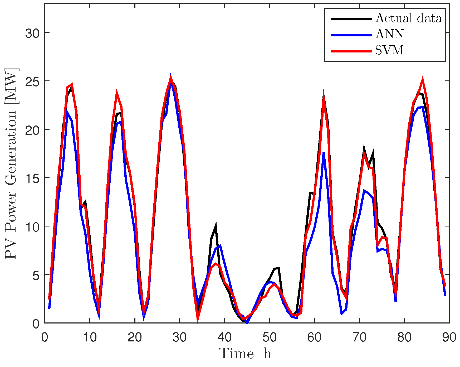
Then, we evaluate the performance of the different prediction schemes by using historical data for DA and RT LMP from the PJM over a 12-month in 2014 [44]. The average DA LMP and RT LMP in 2014 are $53.76/MWh and $52.72/MWh, respectively. In addition, the DA bids due is 12 a.m., and we assume that PV power producers can submit RT re-bids at 1-hour ahead of the operating hour.

5.1. ESS Sizing for Machine Learning Prediction Schemes

In this section, three different power capacities of the ESS, $P_{ESS}$, are considered for absorbing the prediction errors. Figure 8 shows the operation of the PCS of the ESS, which utilizes the ANN scheme for varying time intervals of day time (7:00 A.M. to 6:00 P.M.) with a $5\%$ tolerance limit of the installed PV capacity. The power output of the PCS of the ESS is obtained in a straightforward calculation from Equations (16) and (17). The ESS power is very frequently charged or discharged in order to reduce the prediction error for the ANN scheme. In addition, it can be inferred that the deviation penalties of the small-sized PCS (5% of the installed PV capacity) would be significantly larger than that of the large-sized PCS (15% of the installed PV capacity) because a large amount of prediction errors is still not absorbed by the ESS in case of 5% of the installed PV capacity. Similarly, the power output of the PCS for the SVM scheme is shown in Figure 9. In case of the SVM scheme, The ESS power is less frequently charged or discharged, compared with that of the ANN scheme and the average power output of the PCS of the ESS is also smaller than that of the ANN scheme. Furthermore, in order to quantitatively compare the amount of exchanged power of ESS between the ANN and SVM schemes, we estimate the average amount of the hourly exchanged power of ESS (${\overline{P}}_{ESS}$), which is calculated as ${\overline{P}}_{ESS}=\frac{1}{N-M}{\sum }_{i=M+1}^N\left|P_i\right|$.

Table 3. The average amount of the hourly exchanged power [kW] of ESS both the ANN and SVM schemes for a 30-MW PV system (Tolerance limit = 5%).

Power Capacity	ANN	SVM
5%	501.56	234.90
10%	707.99	301.80
15%	793.95	322.45

summarizes the average amount of the hourly exchanged power of ESS both the ANN and SVM schemes for a 30-MW PV system. This result also shows that the average amount of the hourly exchanged power of ESS for the SVM scheme is smaller than that of the ANN scheme for three different power capacities of the ESS. In addition, compared with the smaller power capacity of ESS for the SVM scheme, the average amount of the hourly exchanged power of the SVM scheme is very slightly increased and most of the prediction errors do not exceed the allowable limit $P^{\prime }$ when the power capacity of the ESS is 15% of the installed PV capacity.

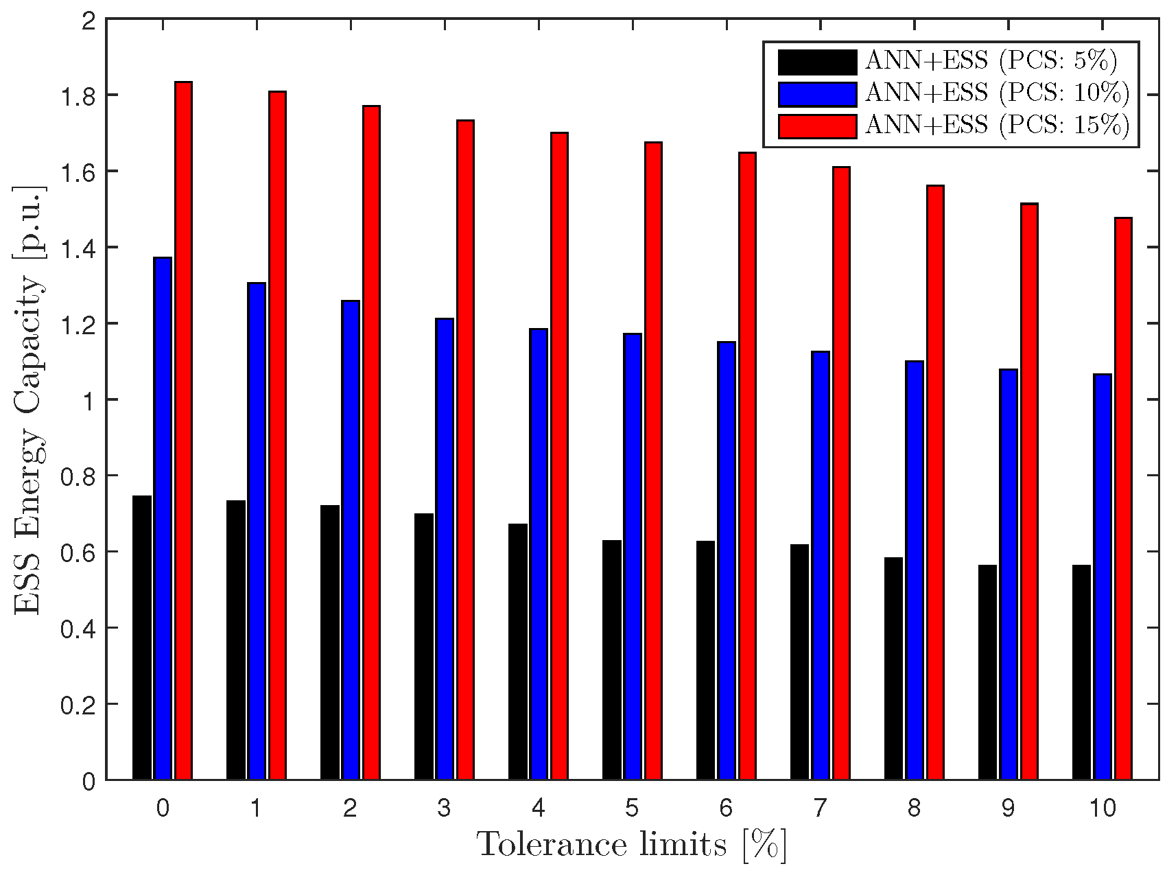
The optimum ESS energy capacity, $E_{ESS}$, has been calculated by Equation (18). Figure 10 shows the energy capacity of the ANN scheme with different tolerance limits. As the power capacity of the ESS $P_{ESS}$ increases, $E_{ESS}$ rapidly becomes larger. On the other hand, the tolerance limit does not have a significant effect on the decrease in $E_{ESS}$ for the ANN scheme because there still exist greater prediction errors than $P_{ESS}$ even if we consider the tolerance limit.

Figure 11 shows the energy capacity of the SVM scheme with different tolerance limits. Most prediction errors of the SVM scheme occur in the small error region (−0.05 to 0.05 [p.u.]), as shown in Figure 4 and a large portion of prediction errors for the SVM scheme is reduced by the tolerance limit. Therefore, as the tolerance limit increases, $E_{ESS}$ gradually becomes smaller.

Table 4. Energy capacity [p.u.] of both the ANN and SVM schemes with different tolerance limits.

Scheme	Power Capacity	0%	2%	4%	6%	8%	10%
	5%	0.74	0.72	0.67	0.63	0.58	0.56
ANN	10%	1.37	1.26	1.19	1.15	1.10	1.07
	15%	1.83	1.77	1.70	1.65	1.56	1.48
	5%	0.62	0.45	0.33	0.28	0.23	0.22
SVM	10%	0.84	0.61	0.51	0.44	0.43	0.34
	15%	0.93	0.78	0.63	0.52	0.45	0.40

summarizes the energy capacity of both of the ANN and SVM schemes with different tolerance limits.

5.2. Assessment of the Profit for the PV Power Producers

Figure 12 shows the hourly deviation penalties for varying tolerance limits with a penalty factor $\alpha$ of 1.0. The hourly deviation penalties have been calculated by Equations (14) and (15) considering the 10% power capacity as a fraction of the 30-MW PV farm. It can be observed that the deviation penalties from the SVM scheme without ESS significantly decrease, compared with those of the ANN scheme without ESS due to high prediction accuracy. The SVM-based prediction scheme without ESS yields a decrease in the deviation penalty by up to 48%, compared with that of the ANN scheme. In addition, the deviation penalties can be quite reduced by using ESS. Since the ESS power is more frequently charged or discharged for the ANN scheme, compared with that of the SVM scheme, as shown in Figure 8, the effect of the ESS for the ANN scheme is greater than that of the SVM scheme in terms of the deviation penalty reduction. Considering the 10% power capacity as a fraction of the 30-MW PV farm, the deviation penalty for using ESS for the ANN and SVM schemes decreases by up to 87% and 74%, respectively.

Table 5. Hourly deviation penalties [$/h] of both ANN and SVM schemes with different power capacities and tolerance limits.

Scheme	Power Capacity	0%	2%	4%	6%	8%	10%
ANN	No ESS	266.27	257.01	231.48	195.38	155.57	117.81
	5%	214.32	175.54	136.16	100.88	70.02	49.95
	10%	117.81	85.59	60.17	41.26	27.80	18.52
	15%	49.95	33.93	22.71	15.07	9.96	6.57
SVM	No ESS	190.99	176.36	143.32	109.05	81.52	61.39
	5%	125.60	94.30	70.62	53.61	41.47	32.71
	10%	61.39	47.03	36.74	29.25	23.69	19.48
	15%	32.71	26.27	21.45	17.76	14.88	12.61

summarizes the hourly deviation penalties [$/h] for both of the ANN and SVM schemes with different power capacities and tolerance limits.

Figure 13 shows the variation of the hourly energy market profit with different tolerance limits and a penalty factor of 1.0. As the tolerance limit $P_{tol}$ increases, the hourly energy market profit for both of the ANN and SVM schemes with ESS gradually approaches the no-penalty market profit ($ 589/h). It implies that a zero deviation penalty would be given to both of the ANN and SVM schemes with ESS when energy markets allow a tolerance limit $P_{tol}$ of larger than 10%.

In Equation (12), the hourly deviation penalties with a tolerance limit of 5% for both of the ANN and SVM schemes increase in proportion to an increase in the penalty factor, as shown in Figure 14. In addition, in high penalty factors, the hourly deviation penalties for both of the ANN and SVM schemes with ESS is negligible, compared with those for both of the ANN and SVM schemes without ESS. As a result, a reasonable selection of the tolerance limit and the penalty factor is required to satisfy the economic feasibility of the PV producers in order to introduce the successful energy market introduction of ESSs. In Section 5.3, we can find the appropriate market policy or parameters for both the ANN and SVM schemes from the benefit-cost analysis (BCA) of PV power trading.

5.3. Benefit-Cost Analysis (BCA) for the ESS in PV Power Trading

The BCA provides the comparison of the total expected cost of against the total expected benefit to confirm whether the benefit outweighs the cost and by how much [45]. In the BCA, the benefit-cost ratio (B-C ratio) is the present value of benefit divided by the present value of cost. In order that a project may be economically feasible, the B-C ratio should be greater than one [46]. The benefit-cost ratio is computed as

$$\begin{array}{c}\hfill B-Cratio=\frac{{\sum }_{i=1}^{T_{life}}\left[B_i·\frac{{(1+r_{IR})}^i}{{(1+r_{RI})}^i)}\right]}{{\sum }_{i=1}^{T_{life}}\left[\frac{C_i}{{(1+r_{RI})}^i)}\right]},\end{array}$$

(19)

where $B_i$ is the benefit in the i-th year and $C_i$ is the cost in the i-th year. Moreover, $T_{life}$ is the life of the project (years) and $r_{RI}$ is the rate of interest (fraction) and $r_{IR}$ is the inflation rate (fraction).

In this paper, $B_i$ represents the profit difference between with/without ESS in the i-th year for BCA in PV power trading. Considering the cost reduction of the ESS, the power system cost ($/kW) is set to $300/kW and the energy storage cost ($/kWh) of the lithium-ion battery is set to $450/kWh [42]. Moreover, we consider the life-time of the project of 10 years, the rate of interest ($r_{RI}$) of 4%, and the inflation rate ($r_{IR}$), the increase rate of electricity price) of 2%.

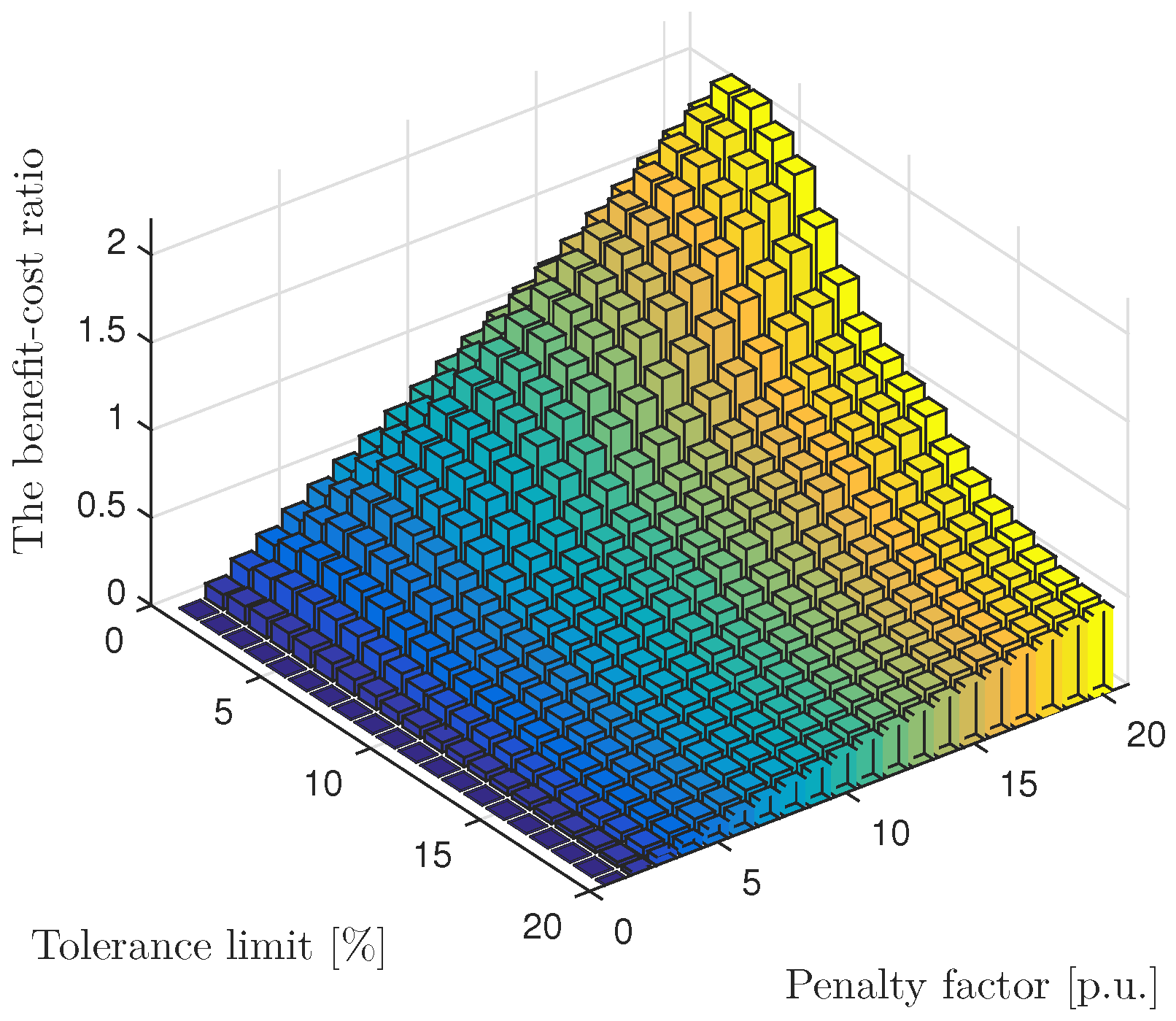
Figure 15 shows the benefit-cost ratio of the ANN scheme with a power capacity of 10% of the installed PV capacity. When the energy market permits a low tolerance limit (≤6%) and a high penalty factor (≥1.9), the benefit-cost ratio of the ANN scheme is greater than one. In other words, there is economical benefit of installing the ESS when the energy market enforces a harsh policy in terms of the tolerance limit and penalty factor for PV power producers. The maximum B-C Ratio of the ANN scheme is 1.1034 in a tolerance limit of 4% and a penalty factor of 2.0.

Figure 16 shows the benefit-cost ratio of the SVM scheme with a power capacity of 10% of the installed PV capacity. The SVM scheme yields a larger benefit-cost ratio than that of the ANN scheme in the same market parameters because the SVM scheme requires a quite smaller amount of the energy capacity of the ESS than the ANN scheme, as shown in Figure 11. When the tolerance limit is smaller than 11% and the penalty factor is larger than 1.0, the benefit-cost ratio of the SVM scheme is greater than one. When PV power producers adopt the SVM scheme for PV output power prediction, they also obtain much higher profit at a hard penalty market than a soft penalty market. Furthermore, the maximum benefit-cost ratio (BCR) value of the SVM scheme is 2.2043 in a tolerance limit of 2% and a penalty factor of 2.0.

Table 6. The maximum benefit-cost ratio (BCR) value of the ANN and SVM schemes for different power capacities of ESSs.

Scheme	Power Capacity	Max. BCR	Tolerance Limit	Penalty Factor
	5%	1.17	6%	2.0
ANN	10%	1.10	4%	2.0
	15%	0.96	3%	2.0
	5%	2.32	4%	2.0
SVM	10%	2.20	2%	2.0
	15%	2.11	2%	2.0

summarizes the maximum BCR value of the ANN and SVM schemes for three different power capacities of ESSs. The smaller power capacity of the ESS has a greater maximum BCR value for each prediction scheme. However, the smaller power capacity of the ESS is not always the best choice because a power capacity of 10% of the installed PV capacity yields a higher maximum BCR value (2.20) than that of a power capacity of 5% of the installed PV capacity (2.02) for the SVM scheme when a tolerance limit of less than 2% is allowed in a specific energy market. Therefore, PV producers need to select the optimal size of the ESS, which has the highest BCR value to absorb the prediction errors, considering the different energy market policies. In addition, it can be observed that the PV power producer’s profit also significantly increases by achieving high accuracy of the prediction scheme.

6. Conclusions

In this paper, it has been shown that the accurate machine learning (ML)-based PV output power prediction schemes with ESS management could significantly increase the market profit of PV power producers. For that purpose, the ANN and SVM schemes were utilized for predicting the PV output power from various meteorological big data. In addition, the capacity of ESSs, which can compensate the prediction error, was estimated from different energy market constraints. And then, we calculated the PV power producer’s profit considering the deviation penalties in case of ML-based prediction schemes with/without ESS in order to quantitatively estimate the effect of ESS for different prediction accuracies of two ML-based prediction schemes. Numerical results were presented as a case study on the participation of a 30-MW PV farm in the LMP market of the PJM. These results showed the SVM scheme without ESS yields a decrease in the deviation penalties by up to 48% than the ANN scheme without ESS. In case of ML-based prediction schemes with ESS, the ANN and SVM schemes yield an decrease in the deviation penalty by up to 87% and 74%, respectively, compared with the profit of the ANN and SVM schemes without ESS. From the benefit-cost analysis (BCA) in the case study, it could be observed that the maximum B-C ratio of PV power producers significantly increases by using a more accurate prediction scheme with ESS and the maximum B-C ratio is 2.32 for the SVM scheme. Furthermore, the BCA results provided the economic regions of market parameters for both of the ANN and SVM schemes. As a result, the proposed ESS-based PV power trading could be suitable for the participation of PV power producers in order to increase the profit in a penalized market.

In this paper, since we utilized the actual meteorological data instead of the forecasted meteorological data, which has already been known in the prediction time, due to a difficulty in obtaining the proper forecasted meteorological data set, the prediction accuracy of the ANN and SVM schemes may slightly degrade in a real environment due to the forecasting accuracy of the meteorological parameters. We need to enhance the prediction scheme by reflecting the forecasted meteorological data for the practicality of prediction in further works.

References

1. Cheng, D.; Mather, B.A.; Seguin, R.; Hambrick, J.; Broadwater, R.P. Photovoltaic (PV) Impact Assessment for Very High Penetration Levels. IEEE J. Photovolt. 2016, 6, 295–300. [Google Scholar] [CrossRef]
2. Korea Ministry of Trade, Industry and Energy. Renewable Energy Statistics. 2013. Available online: http://www.motie.go.kr (accessed on 20 February 2019).
3. Jang, H.S.; Bae, K.Y.; Park, H.-S.; Sung, D.K. Effect of aggregation for multi-site photovoltaic (PV) farms. In Proceedings of the IEEE International Conference on Smart Grid Communications (SmartGridComm), Miami, FL, USA, 2–5 November 2015; pp. 623–628. [Google Scholar]
4. Tewari, S.; Geyer, C.J.; Mohan, N. A statistical model for wind power forecast error and its application to the estimation of penalties in liberalized markets. IEEE Trans. Power Syst. 2011, 26, 2031–2039. [Google Scholar] [CrossRef]
5. DeMeo, E.A.; Jordan, G.A.; Kalich, C.; King, J.; Milligan, M.R.; Murley, C.; Oakleaf, B.; Schuerger, M.J. Accommodating wind’s natural behavior. IEEE Power Energy Mag. 2007, 5, 59–67. [Google Scholar] [CrossRef]
6. Kraas, B.; Schroedter-Homscheidt, M.; Madlener, R. Economic merits of a state-of-the-art concentrating solar power forecasting system for participation in the Spanish electricity market. Sol. Energy 2013, 93, 244–255. [Google Scholar] [CrossRef]
7. Marquez, R.; Coimbra, C.F. Intra-hour DNI forecasting based on cloud tracking image analysis. Sol. Energy 2013, 91, 327–336. [Google Scholar] [CrossRef]
8. Jang, H.S.; Bae, K.Y.; Park, H.S.; Sung, D.K. Solar power prediction based on satellite images and support vector machine. IEEE Trans. Sustain. Energy 2016, 7, 1255–1263. [Google Scholar] [CrossRef]
9. Perez, R.; Kivalov, S.; Schlemmer, J.; Hemker, K.; Renné, D.; Hoff, T.E. Validation of short and medium term operational solar radiation forecasts in the US. Sol. Energy 2010, 84, 2161–2172. [Google Scholar] [CrossRef] [Green Version]
10. Lorenz, E.; Hurka, J.; Heinemann, D.; Beyer, H.G. Irradiance forecasting for the power prediction of grid-connected photovoltaic systems. IEEE J. Sel. Top. Appl. Earth Obs. Remote Sens. 2009, 2, 2–10. [Google Scholar] [CrossRef]
11. Torres, J.L.; Garcia, A.; De Blas, M.; De Francisco, A. Forecast of hourly average wind speed with ARMA models in Navarre (Spain). Sol. Energy 2005, 79, 65–77. [Google Scholar] [CrossRef]
12. Reikard, G. Predicting solar radiation at high resolutions: A comparison of time series forecasts. Sol. Energy 2009, 83, 342–349. [Google Scholar] [CrossRef]
13. Li, Y.; Su, Y.; Shu, L. An ARMAX model for forecasting the power output of a grid connected photovoltaic system. Renew. Energy 2014, 66, 78–89. [Google Scholar] [CrossRef]
14. Amrouche, B.; Le Pivert, X. Artificial neural network based daily local forecasting for global solar radiation. Appl. Energy 2014, 130, 333–341. [Google Scholar] [CrossRef]
15. Bae, K.Y.; Jang, H.S.; Sung, D.K. Hourly solar irradiance prediction based on support vector machine and its error analysis. IEEE Trans. Power Syst. 2017, 32, 935–945. [Google Scholar] [CrossRef]
16. Yang, H.-T.; Huang, C.-M.; Huang, Y.-C.; Huang, Y.-S. A weather-based hybrid method for 1-Day ahead hourly forecasting of PV power output. IEEE Trans. Sustain. Energy 2014, 5, 917–926. [Google Scholar] [CrossRef]
17. Ji, W.; Chee, K.C. Prediction of hourly solar radiation using a novel hybrid model of ARMA and TDNN. Sol. Energy 2011, 85, 808–817. [Google Scholar] [CrossRef]
18. Lorenz, E.; Hurka, J.; Heinemann, D.; Beyer, H.G. The Federal Energy Regulatory Commission Order No. 764; United States of America Federal Energy Regulatory Commission: Washington, DC, USA, 2012.
19. Botterud, A.; Wang, J.; Miranda, V.; Bessa, R.J. Wind power forecasting in US electricity markets. The Electr. J. 2010, 23, 71–82. [Google Scholar] [CrossRef]
20. Pinson, P.; Chevallier, C.; Kariniotakis, G.N. Trading wind generation from short-term probabilistic forecasts of wind power. IEEE Trans. Power Syst. 2007, 22, 1148–1156. [Google Scholar] [CrossRef]
21. Liang, J.; Grijalva, S.; Harley, R.G. Increased wind revenue and system security by trading wind power in energy and regulation reserve markets. IEEE Trans. Sustain. Energy 2011, 2, 340–347. [Google Scholar] [CrossRef]
22. Botterud, A.; Zhou, Z.; Wang, J.; Bessa, R.J.; Keko, H.; Sumaili, J.; Miranda, V. Wind power trading under uncertainty in LMP markets. IEEE Trans. Power Syst. 2012, 27, 894–903. [Google Scholar] [CrossRef]
23. Bludszuweit, H.; Domínguez-Navarro, J.A.; Llombart, A. Statistical analysis of wind power forecast error. IEEE Trans. Power Syst. 2008, 23, 983–991. [Google Scholar] [CrossRef]
24. Omran, W.A.; Kazerani, M.; Salama, M. Investigation of methods for reduction of power fluctuations generated from large grid-connected photovoltaic systems. IEEE Trans. Energy Convers. 2011, 26, 318–327. [Google Scholar] [CrossRef]
25. Elsied, M.; Oukaour, A.; Gualous, H.; Hassan, R. Energy management and optimization in microgrid system based on green energy. Energy 2015, 84, 139–151. [Google Scholar] [CrossRef]
26. Ma, L.; Liu, N.; Zhang, J.; Tushar, W.; Yuen, C. Energy management for joint operation of CHP and PV prosumers inside a grid-connected microgrid: A game theoretic approach. IEEE Trans. Ind. Inf. 2016, 12, 1930–1942. [Google Scholar] [CrossRef]
27. Kalogirou, S.A. Artificial neural networks in renewable energy systems applications: A review. Renew. Sustain. Energy Rev. 2001, 5, 373–401. [Google Scholar] [CrossRef]
28. Ramadhas, A.S.; Jayaraj, S.; Muraleedharan, C.; Padmakumari, K. Artificial neural networks used for the prediction of the cetane number of biodiesel. Renew. Energy 2006, 31, 2524–2533. [Google Scholar] [CrossRef]
29. MacKay, D.J. Information Theory, Inference and Learning Algorithms; Cambridge university press: Cambridge, UK, 2003. [Google Scholar]
30. Hagan, M.T.; Menhaj, M.B. Training feedforward networks with the Marquardt algorithm. IEEE Trans. Neural Netw. 1994, 5, 989–993. [Google Scholar] [CrossRef] [PubMed]
31. Cortes, C.; Vapnik, V. Support-vector networks. Mach. Learn. 1995, 20, 273–297. [Google Scholar] [CrossRef] [Green Version]
32. Drucker, H.; Burges, C.J.; Kaufman, L.; Smola, A.; Vapnik, V. Support Vector Regression Machines. Adv. Neural Inf. Process. Syst. 1997, 9, 155–161. [Google Scholar]
33. Shi, J.; Lee, W.-J.; Liu, Y.; Yang, Y.; Wang, P. Forecasting power output of photovoltaic systems based on weather classification and support vector machines. IEEE Trans. Ind. Appl. 2012, 48, 1064–1069. [Google Scholar] [CrossRef]
34. Chang, C.-C.; Lin, C.-J. LIBSVM: A library for support vector machines. ACM Trans. Intell. Syst. Technol. (TIST) 2011, 2, 27. [Google Scholar] [CrossRef]
35. Korea Meteorological Administration (KMA). Available online: http://web.kma.go.kr/eng/ (accessed on 20 February 2019).
36. Jackman, S. Bayesian Analysis for the Social Sciences; John Wiley & Sons: Hoboken, NJ, USA, 2009. [Google Scholar]
37. Balanda, K.P.; MacGillivray, H. Land drainage: Planning and design of agricultural systems. Am. Stat. 1998, 42, 111–119. [Google Scholar]
38. Chen, C.; Duan, S.; Cai, T.; Liu, B.; Hu, G. Optimal allocation and economic analysis of energy storage system in microgrids. IEEE Trans. Power Electron. 2011, 26, 2762–2773. [Google Scholar] [CrossRef]
39. Stoft, S. Power system economics. J. Energy Lit. 2002, 8, 94–99. [Google Scholar]
40. Jones, L.E. Renewable Energy Integration: Practical Management of Variability, Uncertainty, and Flexibility in Power Grids; Academic Press: Cambridge, MA, USA, 2014. [Google Scholar]
41. Papalexopoulos, A.D.; Andrianesis, P.E. Performance-based pricing of frequency regulation in electricity markets. IEEE Trans. Power Syst. 2014, 29, 441–449. [Google Scholar] [CrossRef]
42. Schoenung, S. Energy Storage Systems Cost Update; Sandia National Laboratories: Albuquerque, NM, USA, 2011.
43. Han, S.; Han, S.; Aki, H. A practical battery wear model for electric vehicle charging applications. Appl. Energy 2014, 48, 1100–1108. [Google Scholar] [CrossRef]
44. Monitoring Analytics LLC. State of the Market Report for PJM; Monitoring Analytics: Norristown, PA, USA, 2015. [Google Scholar]
45. David, R.; Ngulube, P.; Dube, A. A cost-benefit analysis of document management strategies used at a financial institution in Zimbabwe: A case study. SA J. Inf. Manag. 2013, 15, 10–11. [Google Scholar] [CrossRef]
46. Smedema, L.K.; Rycroft, D.W. Land Drainage: Planning and Design of Agricultural Systems; HarperCollins Distribution Services: London, UK, 1983. [Google Scholar]
Figure 1. Research workflow of ESS-based PV power trading.
Energies 12 01249 g001
Figure 2. A typical structure of a feed-forward ANN network.
Energies 12 01249 g002
Figure 3. Results of PV power prediction of day time for eight consecutive days.
Energies 12 01249 g003
Figure 4. PDFs of the prediction errors for the ANN and SVM schemes.
Energies 12 01249 g004
Figure 5. Market operation timeline.
Energies 12 01249 g005
Figure 6. Estimation of three different positive deviations for charging the ESS.
Energies 12 01249 g006
Figure 7. Estimation of three different negative deviations for discharging the ESS.
Energies 12 01249 g007
Figure 8. Operation of the ESS for the ANN scheme with varying time intervals of day time (Tolerance limit = 5%).
Energies 12 01249 g008
Figure 9. Operation of the ESS for the SVM scheme with varying time intervals of day time (Tolerance limit = 5%).
Energies 12 01249 g009
Figure 10. Energy capacity of the ANN scheme with different tolerance limits.
Energies 12 01249 g010
Figure 11. Energy capacity of the SVM scheme with different tolerance limits.
Energies 12 01249 g011
Figure 12. Hourly deviation penalties with a penalty factor of 1.0.
Energies 12 01249 g012
Figure 13. Hourly energy market profit with a penalty factor of 1.0.
Energies 12 01249 g013
Figure 14. Hourly deviation penalty with a tolerance limit of 5%.
Energies 12 01249 g014
Figure 15. The benefit-cost ratio of the ANN scheme with a power capacity of 10%.
Energies 12 01249 g015
Figure 16. The benefit-cost ratio of the SVM scheme with a power capacity of 10%.
Energies 12 01249 g016