Abstract
The term “energy efficiency” covers a wide scope and it is affected by a lack of clarity. To overcome this issue, quantitative measures should be defined and evaluated for each unit of product or process considered. These quantitative indicators are necessary to support and evaluate energy efficiency improvements in industry, by allowing to (i) monitor the energy performance, and (ii) perform benchmarking analyses with best available techniques or similar processes. The specific energy consumption (SEC), i.e., the amount of energy consumed per unit of product/output, is the most commonly used index. Because of the uncertain demand faced by companies, production processes run at a rate that can vary within a certain range, to which correspond a different utilization of plants. Energy efficiency investments can be categorized in accordance to how they affect the SEC: i.e., the first group of investments has the same effects for each production rate (e.g., replacement of dated electric motors with new technologies), while the other has different effects for different ranges of production rate (e.g., installation of an inverter). The present work proposes a novel decision model for supporting the evaluation of the more suitable energy efficiency investment in an industrial context where the demand is uncertain. A numerical example based on a case study from the aluminum industry is then proposed in order to highlight the relevance of the problem discussed and to evaluate the behavior of the models in different scenarios characterized by different load factors. From the results, it evinced that the return of the investment strongly depends on the range of production rate and, thus, on the demand variability.
1. Introduction
The European Commission recognized energy efficiency as one of the most relevant means in order to reach a sustainable energy future by allowing the reduction of the energy consumptions and of the greenhouse-gas (GHG) emissions, and the enhanced security and reliability of the energy supply [1]. Moreover, the measures aiming at improving the energy efficiency lead to many other benefits that can address social, financial, legal, and competitiveness issues [2]. The potential impact is relevant especially in the industrial sector which uses more delivered energy than any other end-use sector. For instance, in the 2016, it was responsible for about 54% of the world’s total delivered energy [3]. In addition, the worldwide industrial sector energy consumption is expected to further increase up to a value of 309 quadrillion British thermal units (Btu) in 2040, by an average of 1.2%/year [3]. The evaluation of the energy performance has become very important for the companies and the society, and emerged as one of the most significant manufacturing decisions because of the rising and volatile energy prices, the new environmental regulations, and the changes in customers’ purchasing behavior keen on “green” and energy efficient products [4,5].
The EU Commission tried to enhance the energy culture in companies and to increase their awareness underlying that “energy is the same as other valuable raw material resources required to run a business—and is not merely an overhead and part of business maintenance. Energy has costs and environmental impacts and needs to be managed well in order to increase the business’ profitability and competitiveness, as well as to mitigate the seriousness of these impacts” [6]. Though, energy is still viewed by the majority of companies as an operational cost instead of a competitive advantage; energy savings are seen as incidental benefits because of other events rather than a central value-generating proposition. In order to start a gradual process of rethinking toward a more energy-efficient acting, the following key drivers have been highlighted by previous studies: i.e., the energy turnaround in Europe through the proposal of stringent targets in the 2030 climate and energy framework which sent strong signals to the market and encouraged private investments [5]; the relevance of energy issue on the strategic objectives of companies, which are costs, time, and quality [5,7]; and the increasing ecological awareness of the final consumers [5,8].
The term “energy efficiency” is widely used referring to the methods for addressing different objectives (e.g., reduction of carbon emissions, enhancement of security of energy supplies, reduction of costs), and it is affected by a lack of clarity. It can mean different things at different times and in different places or circumstances. A possible way to overcome this lack of clarity is represented by the introduction of key performance indicators (KPIs). The main purpose of the energy efficiency indicators is to be able to monitor the progress of the energy efficiency improvement measures and projects on the energy performance of the company and to perform benchmarking with similar processes or with best available techniques (BAT). Energy efficiency was defined in the EuP Directive 2005/32/EC as “a ratio between an output of performance, service, goods or energy, and an input of energy.” The indicator mostly used is the specific energy consumption (SEC), i.e., the ratio between the total energy consumption and the physical or economic output value, or, in other words, the amount of energy consumed per unit of output [6]. This energy indicator presents several advantages, such as the direct correlation to the process operations and technology, and the insensitivity to price fluctuations. However, a comparison of the energy performance of different units and aggregate efficiency is possible only after a conversion of the physical units into a common economic value [9].
The energy consumption profile of industrial plants is usually given by two contributions [10]: one is constant given the production plant (e.g., energy for auxiliary equipment), while the other is variable depending on the production rate (e.g., energy to run machineries for production requirements). As a consequence, the amount of energy consumed per unit of product, i.e., the specific energy consumption, decreases with an increase of the production rate, as the incidence of the fixed share decreases. The reduction of the SEC because of an increased production rate is quite normal and it is mainly caused by two factors [6]. First, the production equipment operates for longer periods and thus the idle periods become shorter. Second, there is a base energy consumption not depending on the utilization of production capacity (e.g., consumption related to the starting up of equipment, to the use of lights and fans, etc.,), which will be spread over more products.
Industrial plants have to face variable, uncertain and intermittent demands (e.g., days with high production and days with no production, alternation of working times and idle times, etc.,). For that reason, the production process is run at a wide range of production rates, and the required flexibility results in reduced energy efficiency and increased costs [11]. Consequently, this range of production rates should be considered when investments in energy efficiency measures (EEMs) are planned. Ref. [12] proposed a framework to characterize such measures, based on 17 attributes grouped according to six categories, such as: economic, energy, environmental, production-related, implementation-related and the possible interaction with other systems. Specifically, the proposed framework allows to share knowledge on EEMs and on the barriers currently hindering their adoption (e.g., economic, competence- related or information-related). Barriers that can be overcome, at least in part, through collaborative practices among different actors, such as supply chain management [13], energy synergies [14], and supply chain finance [15].
From industrial evidences, two investment options can be defined while considering the effect on the SEC: (i) Investments that have the same impact in reducing the SEC for all the production rates with a relevant expenditure (e.g., substitution of dated equipment), and (ii) investments that differently reduce the SEC for different production rate with organizational improvements (e.g., dispatching rules) or less expensive effort on technologies (e.g., installation of inverters). For instance, [16] investigated the economic feasibility of reducing electric motor electricity consumption in the Korean manufacturing sector through different strategies: e.g., improving the performances of the motor through the increase of the load factor (i.e., reducing the oversizing of the equipment) or enabling the motor to better match the requirements of the process through the installation of variable sped drivers. While, [17] proposed a life cycle cost model for comparing the economic performance of improving the energy efficiency of an electric arc furnace transformer by investing in replacing or revamping the dated technology and implementing intangible services (e.g., maintenance activities, operational consultancy).
In order to evaluate and compare the alternative investment options, the net present value (NPV) approach has been used as it gives better results and allows to compare investments with different characteristics and durations [18]. This work aims to identify the most suitable investment option in energy efficiency and the optimal amount of capital invested capable to maximize the expected NPV, for a given industrial plant under constant and uncertain demand profiles. The remainder of the paper is organized as follows: Section 2 introduces the notations and assumptions and the mathematical model for the different investment options; Section 3 provides numerical examples to illustrate the proposed models; and, finally, Section 4 concludes the paper summarizing the main findings and providing suggestions for future research.
2. Methodology
In this section, two models are provided for evaluating the optimal amount that should be invested aiming at identifying the most suitable investment in improving the energy efficiency with the focus on a single manufacturing company. In Scenario 1, the demand rate faced by the industrial plant, and consequently the production rate, is assumed to be constant. Then, an uncertain demand profile is considered and, hence, the production rate is subject to variations (Scenario 2). In those circumstances, the decision-maker has to establish if it is better to incur in higher expenditures while reducing the specific energy consumption over the interested range of production rates (“SEC reduction”), or in less expensive investment to reduce the variability decreasing the SEC while the equipment is underused (“SEC levelling”).
First, the notation and the assumptions of the model are defined (Section 2.1). Then, in Section 2.2, two models are formulated: i.e., with a constant (Scenario 1) and a stochastic (Scenario 2) demand rate. For the model with a constant demand rate, after having demonstrated the existence of an optimal value, the optimization procedures are provided through an analytical approach which allows to obtain a closed-solution or through the implementation of a step-by-step algorithm, depending on the investment considered.
2.1. Assumptions and Notation
The notation used in the model are:
| Annual demand rate (unit/year) | |
| Actual production rate (unit/h) | |
| Nominal production rate (unit/h) | |
| Investment’s lifespan (years) | |
| Subscript identifying the considered year, | |
| Sensitivity coefficient on the constant of the SEC curve without investment (kWh h/unit2) | |
| Sensitivity coefficient on the exponential of the SEC curve without investment | |
| Sensitivity coefficient on the constant of the SEC curve (kWh h/unit2) | |
| Sensitivity coefficient on the exponential of the SEC curve | |
| Energy cost per unit of production before investment (€/unit) | |
| Energy cost per unit of production after investment (€/unit) | |
| Energy price per kWh (€/kWh) | |
| Specific energy consumption before investment (kWh/unit) | |
| Specific energy consumption after investment (kWh/unit) | |
| Savings introduced with investments (€/year) | |
| Discount rate (%) | |
| Decrease coefficient in the constant of the SEC per € increase in the investment | |
| Decrease coefficient in the exponential of the SEC per € increase in the investment | |
| Investment made to reduce the SEC equally for every production rate (decision variable) (€) | |
| Investment made to reduce the SEC in different way for different production rates (decision variable) (€) |
The main assumptions of the model are the following:
- The demand rate is constant in Scenario 1, while uncertain and, thus, modelled with a stochastic distribution in Scenario 2.
- The operation of the plant is set on a rate, , which is lower than the nominal production rate, , and greater than the demand rate, . Because of the underuse (i.e., ), inefficiencies are introduced, and, consequently, the performance of the plant is worse than the nominal one which means higher energy consumption.
- A lot-for-lot policy is assumed, i.e., the annual demand faced by the company corresponds to the effective production rate multiplied for the hours of operation.
- Stock-outs or shortages are not allowed.
- The SEC of the production process can be approximated and defined as a power function of the production rate, , as follows [19]:
- The energy price per kWh, (€/kWh) is constant over the period considered.
- The investments are mutually exclusive.
- A logarithmic investment function is used to describe the effects of the investments on the parameters of the SEC, due to the diminishing marginal contribution of investments [20,21,22]:where identifies the parameter defining the SEC affected by the investment (i.e., “” or “”), while the investment option.
2.2. Model Formulation
The developed model considers a single firm that has to select the optimal amount of capital that should be invested in energy efficiency in order to maximize the net present value, when facing a range of possible production rate, as he wants to satisfy the uncertain demand through a lot-for-lot policy. Specifically, he can invest in two different options which have different effects in reducing the specific energy consumption curve, i.e., “SEC reduction” which reduces in the same way the SEC at every production rate, and “SEC levelling” which introduces higher reduction for lower production rates levelling the SEC curve. As it is defined in traditional capital budgeting investment decisions, the investment is profitable when the discounted sum of savings, , introduced with the reduction of the unit cost due to the lower specific energy consumption, is greater than the investment cost, . The NPV allows to estimate the net financial benefit provided by the investment undertaken to the company [18], and can be defined as follows:
where , and .
In the equations below, the different effects on the SEC of the two investments option are defined. In Equations (4) and (5), “SEC reduction” investment () affects only the constant of the SEC curve (i.e., parameter ). On the contrary, in Equations (6) and (7), “SEC levelling” investment () reduces the slope of the SEC curve () while maintaining unchanged SEC for the maximum production rate, .
First, in Section 2.2.1, the demand rate is considered constant, evaluating the optimal investment decision for a given value of the production rate (Scenario 1). Then, in Section 2.2.2, it is considered uncertain and modelled with a stochastic distribution leading to a variable production rate (Scenario 2). As the investments are mutually exclusive, the analysis of the optimal invested capital amounts can be done separately.
2.2.1. Scenario with Constant Demand
In Scenario 1, the demand is assumed to be constant over the time period. Given Equations (4)–(7), the NPV for “SEC reduction” and “SEC levelling” are defined in Equations (8) and (9), respectively.
Through the study of the derivatives of the NPV with respect to the invested amount, for both the investment options (i.e., Equations (10)–(12) for the “SEC reduction” scenario and Equations (13) and (14) for the “SEC levelling” scenario), it is possible to demonstrate the convexity of the NPV and thus the existence of an optimal value for the amount of capital that the firm has to invest ().
While for the scenario with the “SEC reduction” investment, it is possible to find a closed solution for the optimal invested amount, as defined in Equation (12); in the “SEC levelling” scenario, it is quite complex to reach. Thus, it can be obtained by implementing the following step-by-step algorithm:
- Step 1.
- Set and .
- Step 2.
- Calculate trough Equation (9).
- Step 3.
- If , then set and go to Step 2, otherwise is the optimal solution.
2.2.2. Scenario with Stochastic Demand
In Scenario 2, the demand rate is uncertain, and this uncertainty affects the production rate. Both the rates are, hence, modelled with stochastic distributions. As a consequence, the savings introduced through the invested capital and the NPV previously obtained are expected values. So, it is not certain that the decision taken will be the best. In this case, it is possible to compare the behavior of two investment options and the respective NPV by evaluating the probability that one NPV is greater than the other, in order to have more precise and detailed results. Specifically, the probability that “SEC levelling” generates higher financial benefits than “SEC reduction,” , is defined in Equation (15).
From industrial evidence, it results that a standard normal distribution can be considered for both the demand and production rates. Hence, also the resulting NPV fits a normal distribution (Figure 1), and the probability defined in Equation (15) becomes [23]:
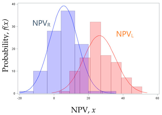
Figure 1.
Probability distributions of the net present value (NPV) for both the investment options.
3. Numerical Study
In the present section, a real case study in the aluminum casting is proposed to investigate the behavior of the model developed and gain some managerial insights. In [24], improvement actions for energy wastes reduction in a die casting company in Italy with a capacity of more than 20,000 tons of aluminum per year have been identified through the use of energy oriented value stream mapping (EO-VSM) tool. Starting from the results of the previous investigation, this case study considers two alternative investment options (i.e., the substitution of dated electric motors with more efficient ones, from IE3 to IE4, and the installation of inverters) to be implemented on some of the production lines, which are a total of 20. The replacement of the main electric motor of the high pressure die casting islands impacts on the energy consumption increasing about 8% of the energy efficiency and reducing the SEC for each production rate. While, the installation of the inverter by adjusting the production speed of the presses of the various high pressure die casting islands allows to modulate the power and, hence, it flattens the SEC curve reducing mostly the energy consumption in condition of underuse (i.e., for lower production rates). The model developed in the previous section can be useful both to investigate the optimal amounts of the alternative solutions and to compare the net present value of two investments with a given investment cost. The parameters used in the numerical example are the following: = 100 unit/h, = 10 year, = 4%, = 0.1 €/kWh, = 145 kWh⋅h/unit2, = 1.13, = 30,000, = 3500. It is also assumed that the plant operates for 2000 h/year.
The data available on the demand rates well fit a normal distribution with mean value = 170,000 unit/h and standard deviation = 500, to which corresponds a normal distribution with mean value = 85 unit/h and standard deviation = 11 as a good approximation for the production rate, given the annual operation time. However, the load factor (LF), i.e., production rate probability distributions, highly affects the financial benefits of the two investment options. Thus, the load factor resulting from the real data (LF1) is compared with two additional load factors with the same standard deviation but with different mean values: i.e., 50 unit/h and 15 unit/h for LF2 and LF3, respectively (see Figure 2). It should be noted that scenario 1 represents a particular case of scenario 2 in which the standard deviation is equal to zero.
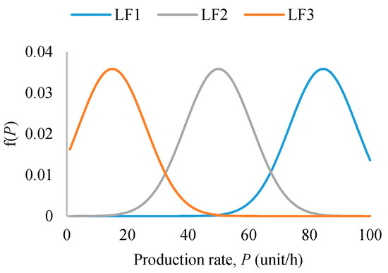
Figure 2.
Load factors considered in the numerical analysis.
The effects of the investments change whereas the demand and production rates are not fixed values but can vary in a range of value according to a stochastic distribution. The probability of occurrence of each rate is used as the weight of the savings introduced with the specific rates in order to determine the total savings and the NPVs. In addition to the NPV, the easier payback period (PB) has been also evaluated since it gives a faster response and fits the managers’ investment decisions-making. The numerical example for scenario 2 characterized by the normal distributions leads to the expected results shown in Table 1.

Table 1.
Expected results of the numerical example for different load factors in scenario 2 if the demand rate follows a normal distribution.
From the results in Table 1, it is possible to gain some insights. First, it can be observed that the NPV is positive in both the scenario for each load factor. Thus, both the investment options are convenient (Figure 3). In particular, the scenario with the investment tending to level the SEC curve leads to a better result than the other investment for lower load factors (LF3). In fact, “SEC levelling” highly reduces the specific energy consumption with respect to the as-is scenario (i.e., scenario without any kind of investment) for low production rates without facing a great expenditure. The effects of this investment option on the SEC is highly dependent on the load factor considered, while “SEC reduction” presents less-variable results. On the contrary, higher load factors (LF1) allow “SEC reduction” to be more convenient, since in this case fewer events of underuse occur. The NPVs for both the investments are lower for higher load factors because of the lower effects of the investments and, consequently, the payback (PB) is higher. The payback periods result in different conclusions, since “SEC levelling” is less expensive than “SEC reduction,” it leads always to shorter PB even if the NPV is lower. Note that for the intermediate load factor (LF2), the NPV of the alternative solutions are closer. “SEC reduction” leads to great energy benefits however the investment cost counterbalance its effects; while “SEC levelling” has lower effects but also lower cost. Moreover, from Figure 3, it is evident that the NPV of “SEC reduction” is subject to lower variance; while, “SEC levelling” has more variable results.
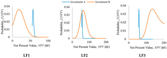
Figure 3.
Probability distributions of the NPV of the two different investment options—“SEC reduction” (Investment A) and “SEC levelling” (Investment B)—under normal distributed demand and production rate.
The profitability of the investments highly depends on the production rate of the production plant. Consequently, an analysis of the behavior of the alternative investment options for different mean values of P should be examined. Lower mean values of the production rate lead to higher expected NPVs (Figure 4a) despite the higher specific energy consumption. This can be explained by the convenience to invest greater capital amount (Figure 4b).
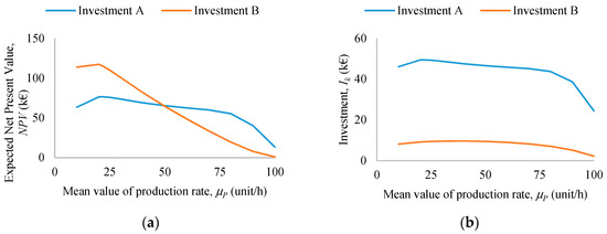
Figure 4.
Effects of variation in the mean value of the production rate on (a) the expected net present value, , and (b) the invested amount, . Legend: Investment A stands for the investment in “SEC reduction,” while Investment B for the “SEC levelling”.
Interesting values of the production rate are the mean values at which the two investments have the same (i) impact on the energy consumption (i.e., equal SEC), and (ii) financial performance (i.e., equal NPV). Above these values, the investment that has higher effects in the reduction of the SEC and better financial performance is “SEC reduction.” If the NPV curves of the two investment options do not intersect, it means that one investment leads to better results for all the range of production rates considered. In the present example, the value at which the effects of the two investment in reducing the SEC is equal is near 21 unit/h; while the same NPV occurs for a production rate of about 50 unit/h. The probability that the NPV of “SEC levelling” in greater the one of “SEC reduction,” as defined in Equation (16), is 0.68%, 48.28%, and 88.24% for LF1, LF2, and LF3 respectively. This probability confirms the previous observation that for lower (higher) load factor, “SEC levelling” (“SEC reduction”) performs better.
Some additional relevant analyses have been carried out in order to consolidate the model’s behavior and to evaluate the significance of several parameters. First, in Figure 5a, the NPV has been estimated by changing the energy price, , since that parameter is frequently variable and policy dependent. The NPV increases for higher values of the energy price, considering both the investment options and all the load factors. For LF1 and LF2, “SEC reduction” is more sensitive to variation in the electricity price and increases its convenience over “SEC levelling” for higher prices. While, if we consider LF3, “SEC levelling” maintains its convenience and the performance gap within the two options remains almost constant. An analysis on the as-is specific energy consumption (i.e., the specific energy consumption before any types of investment, ) has also been performed by varying the coefficients (Figure 5b) and (Figure 5c). Changes in both the coefficients of the SEC have higher effects on the “SEC reduction.” In addition, in both the analyses, higher (higher and lower ) increases the NPV and, thus, the convenience of the investments. Note that the convenience of one investment against the other is different for different parameters’ value; e.g., for very low values of “SEC levelling” is more convenient than “SEC reduction” for each load factor.
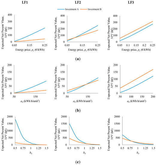
Figure 5.
Variations in the net present value of the two investment options—“SEC Reduction” (Investment A) and “SEC levelling” (Investment B)—for each load factor by changing: (a) the energy price, , (b) the coefficient , and (c) the coefficient of the specific energy consumption without any investment.
Another interesting analysis can be carried out considering an annual variation of the demand rate. Specifically, in the following analysis, it has been considered that the demand rate is not constant over the years, but it is subject to a constant rate of growth/decrease every year. From Figure 6, it is possible to observe that the benefits introduced with the investments are greater if the demand rate is characterized by a positive annual variation. Considering the intermediate load factor (LF2), “SEC levelling” is more convenient for decreased demand rates through the years, while “SEC reduction” for positive variations. Moreover, “SEC reduction” generates an NPV that increases with a higher rate than the alternative investment option.
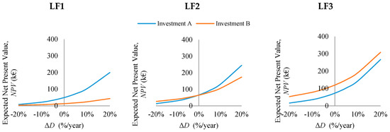
Figure 6.
Effects on the NPV of both the investment options—“SEC reduction” (Investment A) and “SEC levelling” (Investment B)—while considering an annual variation of the demand rate.
The parameters defining the logarithmic function that evaluates the effects of the investments on the SEC (i.e., and ) highly influences the results. Figure 7 shows the effects on the NPV of variations in , and for the three load factors. Higher values of both the parameters, which mean higher investment costs, lead to lower NPV and lower invested amounts.
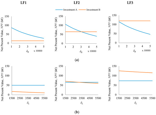
Figure 7.
Sensitivity analysis on the expected NPV of the investments in “SEC reduction” (Investment A), and “SEC levelling” (Investment B) for the different load factors with respect to the parameters of the logarithmic investment function: i.e., (a) , and (b) .
The last sensitivity analysis evaluates how different variability of the production rate (i.e., different standard deviation, ) affects the results of the investment. A higher variability of the production rate increases the convenience of “SEC levelling” with respect to “SEC reduction,” since it leads to a flattened SEC curve influencing the SEC of a wider range of production rates. In Figure 8, the NPV for different standard deviations of the normal distribution defining the production rate, is presented for the three load factors. The NPV of LF2 is less affected by the variations in the standard deviation.
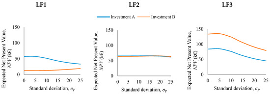
Figure 8.
Expected NPV of the investments in “SEC reduction” (Investment A) and “SEC levelling” (Investment B) for different standard deviation values of the normal distributions defining the production rate for the three load factors investigated.
4. Conclusions
Taking into account the energy demand in an industrial process, two contributions can be distinguished: one fixed and one variable with respect to the production rate. As a direct consequence, the SEC decreases for increased production rate. This aspect is relevant since usually the demand that industrials plants has to face is variable and uncertain and, thus, the production rate does not correspond to a fixed value but covers a wide range of values. The aim of the present work is to propose a novel decision model to support the evaluation of the more suitable energy efficiency investment option and the more profitable amount while considering a stochastic demand that defines its uncertainty. Specifically, two alternative investment options have been considered which have a different impact on the SEC curve. A first option (“SEC reduction”) has the same effects in reducing the SEC for all the production rate and can be implemented only with an expensive expense (e.g., change of technologies). The other option (“SEC levelling”) has different effects for different values of production rate and can be usually obtained with a less expensive effort (e.g., installation of inverters for modulating the equipment use, organizational improvement). The main field of application, in which the proposed models can be more beneficial, is the energy-intensive industries (e.g., metal, pulp and paper, etc.) facing an uncertain production rate.
The numerical example proposed considers a specific case study, hence, the results has no aim of generalization. They allow to highlight the relevance of the problem discussed and to evaluate the behavior of the models in different scenarios characterized by different load factors. The analyses show that both the investment options are convenient in the lifetime considered and generate energy cost savings. Moreover, it evinced that the return of the investment strongly depends on the range of production rate and, thus, on the demand variability. When the variability of the production rate is high, the investment option which leads to a flatter SEC curve (“SEC levelling”) acquires greater relevance than in the scenarios where the uncertainty and the variability are lower.
One of the main limits of the models is the assumption of the continuity and possibility of differentiating the NPV function. In industrial practice, NPV is not a continuous function, as the cost of capital expenditure is affected by relevant and unpredictable variations. This limitation can be overcome by assuming an uncertain capital cost. A further development of the present study may concern the opportunity to implement both the investment options and to evaluate the joint effects, by relaxing the assumption of mutual exclusiveness. Finally, the study focused on the direct energy consumption related to production machines while the contributions of auxiliary and indirect systems is not considered. To address this issue the energy value stream mapping approach can be used [24].
Author Contributions
Conceptualization, B.M. and S.Z.; methodology, B.M.; writing—original draft, B.M.; writing—review and editing, S.Z. and I.F. All authors have read and agreed to the published version of the manuscript.
Funding
This research received no external funding.
Conflicts of Interest
The authors declare no conflict of interest.
References
- International Energy Agency. World Energy Investment Outlook; International Energy Agency: Paris, France, 2003; Volume 23, p. 329. [Google Scholar] [CrossRef]
- Brun, L.; Gereffi, G. The Multiple Pathways to Industrial Energy Efficiency; Report 2011; Global Value Chains (GVC) Center, Duke University: Durham, NC, USA, 2011. [Google Scholar]
- International Energy Outlook 2016; U.S. Energy Information Administration: Washington, DC, USA, 2016; Volume 0484, ISBN 2025866135.
- Zavanella, L.E.; Marchi, B.; Zanoni, S.; Ferretti, I. Energy considerations for the economic production quantity and the joint economic lot sizing. J. Bus. Econ. 2019, 89, 845–865. [Google Scholar] [CrossRef]
- Bunse, K.; Vodicka, M.; Schönsleben, P.; Brülhart, M.; Ernst, F.O. Integrating energy efficiency performance in production management—Gap analysis between industrial needs and scientific literature. J. Clean. Prod. 2011, 19, 667–679. [Google Scholar] [CrossRef]
- European Commission. Reference Document on Best Available Techniques for Energy Efficiency; European IPPC Bureau: Seville, Spain, 2009. [Google Scholar]
- Müller, E.; Poller, R.; Hopf, H.; Krones, M. Enabling Energy Management for Planning Energy-efficient Factories. Procedia CIRP 2013, 7, 622–627. [Google Scholar] [CrossRef]
- Wang, D.; Li, S.; Sueyoshi, T. DEA environmental assessment on U.S. industrial sectors: Investment for improvement in operational and environmental performance to attain corporate sustainability. Energy Econ. 2014, 45, 254–267. [Google Scholar] [CrossRef]
- Assessing Measures of Energy Efficiency Performance and Their Application in Industry; International Energy Agency: Paris, France, 2008.
- Gutowski, T.; Dahmus, J.; Thiriez, A. Electrical Energy Requirements for Manufacturing Processes. In Proceedings of the 13th CIRP International Conference Life Cycle Engineering, Leuven, Belguim, 31 May–2 June 2006; pp. 1–5. [Google Scholar]
- Faccio, M.; Gamberi, M. Energy saving in case of intermittent production by retrofitting service plant systems through inverter technology: A feasibility study. Int. J. Prod. Res. 2014, 52, 462–481. [Google Scholar] [CrossRef]
- Trianni, A.; Cagno, E.; De Donatis, A. A framework to characterize energy efficiency measures. Appl. Energy 2014, 118, 207–220. [Google Scholar] [CrossRef]
- Marchi, B.; Zanoni, S. Supply chain management for improved energy efficiency: Review and opportunities. Energies 2017, 10, 1618. [Google Scholar] [CrossRef]
- Marchi, B.; Zanoni, S.; Zavanella, L.E. Symbiosis between industrial systems, utilities and public service facilities for boosting energy and resource efficiency. Energy Procedia 2017, 128, 544–550. [Google Scholar] [CrossRef]
- Marchi, B.; Zanoni, S.; Ferretti, I.; Zavanella, L.E. Stimulating investments in energy efficiency through supply chain integration. Energies 2018, 11, 858. [Google Scholar] [CrossRef]
- Han, J.; Yun, S.J. An analysis of the electricity consumption reduction potential of electric motors in the South Korean manufacturing sector. Energy Effic. 2015, 8, 1035–1047. [Google Scholar] [CrossRef]
- Marchi, B.; Zanoni, S.; Mazzoldi, L.; Reboldi, R. Product-service System for Sustainable EAF Transformers: Real Operation Conditions and Maintenance Impacts on the Life-cycle Cost. Procedia CIRP 2016, 47, 72–77. [Google Scholar] [CrossRef]
- Jackson, J. Promoting energy efficiency investments with risk management decision tools. Energy Policy 2010, 38, 3865–3873. [Google Scholar] [CrossRef]
- Zanoni, S.; Bettoni, L.; Glock, C.H. Energy implications in the single-vendor single-buyer integrated production inventory model. IFIP Adv. Inf. Commun. Technol. 2013, 397, 57–64. [Google Scholar] [CrossRef]
- Beaumont, N.J.; Tinch, R. Abatement cost curves: A viable management tool for enabling the achievement of win-win waste reduction strategies? J. Environ. Manag. 2004, 71, 207–215. [Google Scholar] [CrossRef] [PubMed]
- Porteus, E.L. Investing in Reduced Setups in the EOQ Model. Manag. Sci. 1985, 31, 998–1010. [Google Scholar] [CrossRef]
- Zanoni, S.; Mazzoldi, L.; Zavanella, L.E.; Jaber, M.Y. A joint economic lot size model with price and environmentally sensitive demand. Prod. Manuf. Res. 2014, 2, 341–354. [Google Scholar] [CrossRef]
- O’Connor, P. Practical Reliability Engineering, 4th ed.; Wiley: Hoboken, NJ, USA, 2002. [Google Scholar]
- Zanoni, S.; Ferretti, I.; Zavanella, L.E. Energy value stream methods with auxiliary systems. Eceee Ind. Summer Study Proc. 2018, 281–291. [Google Scholar]


© 2019 by the authors. Licensee MDPI, Basel, Switzerland. This article is an open access article distributed under the terms and conditions of the Creative Commons Attribution (CC BY) license (http://creativecommons.org/licenses/by/4.0/).