Optimal Municipal Energy System Design and Operation Using Cumulative Exergy Consumption Minimisation

Abstract

In developed countries like Austria the renewable energy potential might outpace the demand. This requires primary energy efficiency measures as well as an energy system design that enables the integration of variable renewable energy sources. Municipal energy systems, which supply customers with heat and electricity, will play an important role in this task. The cumulative exergy consumption methodology considers resource consumption from the raw material to the final product. It includes the exergetic expenses for imported energy as well as for building the energy infrastructure. In this paper, we determine the exergy optimal energy system design of an exemplary municipal energy system by using cumulative exergy consumption minimisation. The results of a case study show that well a linked electricity and heat system using heat pumps, combined heat power plants and battery and thermal storages is necessary. This enables an efficient supply and also provides the necessary flexibilities for integrating variable renewable energy sources.

1. Introduction

Recent studies for Austria showed that the available potential for renewable energy sources (RES) is smaller than the current demand [1,2]. To reach the goal of a fully climate neutral society, imports of RES from other countries or local efficiency measures are necessary. In this context, exergy is a useful concept for identifying efficiency potentials. Although energy is subject to the law of conservation and can never be created or destroyed, exergy is the maximum useful work that can be extracted from a form of energy. It is consumed when brought to equilibrium with its surroundings, therefore it is a potential which describes the ability to cause change. It is the motive force that determines the flow of energy and it constantly deteriorates on its way through the energy system [3]. In the literature, there exist a variety of tools and methods [4,5] to identify and reduce exergy destruction and exergy losses. Their main aim is to increase resource efficiency.

The various forms of energy have different exergy contents, e.g., electricity is pure exergy, whereas low temperature heat has a very low exergy content. Most of today’s used (fossil) energy carriers have a high exergy content. Data for 2016 shows that 50.7% of the final energy consumption in Austria is used for heat applications [6]. 66.1% of the heat is used for low temperature applications like domestic heating, hot water or air conditioning. The rest is used for steam or in furnaces in high temperature industrial applications. In a number of energy strategies of highly developed countries, the focus is on decarbonising the electric power generation [7], even though in the OECD member countries only 22.2% of the final energy consumption is electricity [8].

A comprehensive decarbonisation of the energy system requires efficiency measures and a replacement of fossil fuels by renewable electricity [9]. In multi-energy systems (MES) several sectors (e.g., electricity, heat and transport) and energy carriers (e.g., electricity, natural gas, biomass) are considered in an integrated approach [10]. The coupling of energy sectors and their infrastructures using suitable technologies (e.g., heat pumps, CHPs, etc.) enables the utilisation of synergies, and provides the necessary flexibility for integrating variable RES. MES can also relieve the strain on the energy transmission and distribution infrastructure [11,12].

Today’s typical way of energy system optimisation often focus solely on the electricity system, mainly aiming at an optimum dispatch of power plants and storages. The well-developed electricity grid makes electricity an easy to transport good and establishes operational competition between the individual electricity producers. The present approach delivers optimum operational strategies for the whole system, but does not investigate its optimum design. For heat the situation is different, as heat supply is a local issue and individual buildings or small heat grids are usually supplied by one or few plants. The main decision regarding energy and exergy consumption of heat supply is made during the system design process, and the technology selection. Therefore the main two research questions which occur when designing an exergy efficient MES, where heat and electricity sectors are linked:

• What is the optimum system design? How can it provide the necessary flexibility options for the integration variable RES?
• How can this system be efficiently operated to always meet the demand?

This calls for a model which combines planning and operational aspects [13]. The cumulative exergy demand (CExC) methodology [14] includes both the above outlined points. Next to the exergy consumed during operation it also considers the exergy consumed to create the energy system’s infrastructure.

In this paper, we present the application of the CExC-minimisation on municipal energy systems. First we present the current research and the relevant literature on exergy analysis and energy system optimisation in Section 2. This is followed by an introduction into the concept of exergy, the CExC methodology and the optimisation approach in Section 3. Section 4 presents the results from applying the methodology on a municipal energy system. We close this paper with a comprehensive discussion of the results in Section 5.

2. State of Research

The term exergy was first mentioned by Rant in 1953 when he described the “technical working capacity” [15]. Today, the concept of exergy is used in different kind of fields in environmental science and technology. In this section, the basics of exergy are first presented and then a literature overview of the current tools and methods of exergy analysis is given.

2.1. Fundamentals: Exergy, Exergy Destruction and Exergy Losses

The first law of thermodynamics describes the energy conservation. The second law indicates the irreversibility of natural processes. This means that in any real process, exergy is consumed and entropy is created. The second law also provides information regarding the convertibility of energy forms and the direction in which a process proceeds. For example, electricity or mechanical work theoretically can be fully converted into any other form of energy, whereas for instance for heat the convertibility depends on the temperature difference. In general, energy E consists of a useful part exergy B and the useless part anergy A.

$$E=B+A$$

(1)

Exergy is the useful work that can be theoretically extracted from a form of energy when it is brought to equilibrium with its ambient conditions. Anergy in contrary cannot conduct any work. A well-known example for anergy is heat at ambient temperature.

Four different forms contribute to the total exergy of a system: potential exergy $B_{pot}$ (system height relative to the environment), kinetic exergy $B_{kin}$ (system velocity relative to the environment), chemical exergy $B_{ch}$ (deviation of the chemical composition to the environment) and physical exergy $B_{ph}$ (deviation of pressure p and temperature $\vartheta$ from the environment $p_0,{\vartheta }_0$) [5]. Potential and kinetic energy are pure exergy; the chemical exergy can be approximated by using the lower heating value [16]. The physical exergy, $B_{ph}$, of a mass, m, can be calculated by the enthalpy, h, and entropy, s, of a system with its p and $\vartheta$ compared to the ambient conditions ($T_0$, $s_0$).

$$B_{ph}=[(h-h_0)-({\vartheta }_{0}s-{\vartheta }_0{s}_0)] · m$$

(2)

Thermodynamic inefficiencies in an energy system are either caused by exergy destruction $B_D$ or exergy losses $B_L$ [17]. A well known example for exergy destruction is the production of hot water by burning natural gas. Irreversible thermodynamic transformations cause exergy destruction $B_D$ by entropy generation $s_{gen}$. For a system with the mass m these irreversibilities can be described by the Guoy–Stodola theorem (Equation (3)). As exergy is always dependent on a reference state; it is usually described by the reference pressure $p_0$ and reference temperature ${\vartheta }_0$. Commonly this reference is the “standard atmosphere”.

$$B_D={\vartheta }_0{s}_{gen} · m$$

(3)

Exergy losses $B_L$ are caused by exergy transfers over the system boundaries. That might be work, heat or physical streams that cannot be further utilised. Examples are heat losses in a district heat network or flue gas exhaust streams from boilers.

2.2. Exergy Analysis: Tools and Methodologies

So far, for exergy analysis several tools and methodologies have been developed [4,5]. Examples are the the cumulative exergy consumption [14], the exergetic cost theory [18,19], thermoeconomics [20] or the extended exergy analysis [21]. They all share the same major goal to help to improve the system design, even though they have different system boundaries. As exergy is the potential to conduct work, it is especially suited as a common base in MES where different energy forms with different exergy contents are compared [16].

Cumulative exergy consumption (CExC) and the exergetic cost methodology extend exergy analysis of a single process beyond its boundaries to include all processes from natural resources to the final product. They both use a “fuel–product concept”, where for any system a fuel exergy and a product exergy can be defined. Their exergetic definitions depend on the requirements of the task [18]. CExC analysis was introduced by Szargut in 1957 [22] and includes all exergetic expenses from raw materials to the final product [23]. The exergetic cost theory was introduced by Valero et al. [18] and is defined as “the sum of exergy contained in all resources entering the supply chain of the selected product or process” [5]. In this case, the term “cost” is the exergetic expenditure and has not monetary relation. Even though both methods use a different formalisation, their results are equivalent [5].

Both methodologies are applied to different fields. Szargut et al. [14] proposed the the CExC method to improve the “cumulative degree of perfection of chemical processes”. Applications in energy conversion deal with an oxy-fuel combustion plant [24], or an organic Rankine cycle for waste heat power generation [25]. Valero et al. [26] applied the exergetic cost theory to the CGAM problem [27] and represented the productive structure explicitly, which allows optimisation at a local level. Lozano and Valero [28] performed an exergetic cost analysis on a steam boiler in a thermal generating station. In this study, the authors analysed variations in the exergetic costs of the total product and their causes in order to draw conclusions on the boiler’s real performance. As seen in Misra et al. [29], the application of exergetic costs to a LiBr/H₂O vapour absorption refrigeration system enables an approximate optimum design configuration.

The CExC-method was also applied to analyse the resource consumption on a larger scale with different countries and societies [30], for example the United States [31] and China [32]. On a city scale, it was applied to compare energy scenarios in the smart city planning of Milan [33]. Waste heat [34] and low temperature district heat systems [35] were also investigated using exergy analyses. Krause et al. [16] carried out optimum power flow calculations for a MES to maximise its operational exergy efficiency. We did not find any recent literature where the CExC- or exergetic cost method was applied on municipal energy systems.

3. Methodology

In this work, we adapt the CExC-method to determine an exergy optimal design of a municipal MES. This requires modelling the energy system, and the assessment of energy as well as materials streams flowing in and out of the system. The optimal system design is reached when the CExC reaches a minimum. Therefore, we need a precisely formulated objective function and to model all the necessary constraints [21].

3.1. Cumulative Exergetic Consumption

CExC includes all exergetic losses and exergy destruction from raw materials or energy carriers to their final utilisation. Therefore, it quantifies the consumption of primary resources embodied in a product or service [23]. In an energy system, the exergy expenditures are stored in the energy imports, the materials necessary to build the infrastructure and the locally produced RES. RES and the imported energy carriers are converted to the desired form of energy to supply the load. Therefore, the services produced are both the load as well as the excess energy (Figure 1).

The imported energy flows may include renewable and nonrenewable sources. For the exergetic assessment of imported and exported energy following assumption are made [23]:

• Raw materials or energy carriers are attributed their reference exergy.
• Pre-treated materials or energy carriers are attributed an exergy content of their raw value and the exergetic expenses for the pretreatments.
• Any energy delivered to the load gets attributed its exergy content.
• Next to the energy produced to meet the load, excess energy might be created (Figure 1). If it can be further used, it is considered using its exergy content.

Therefore, for energy and material flows, we have to differentiate between their exergy content and their CExC. The exergy content B of an energy stream is the sum of its embodied physical, chemical, kinetic and potential exergy.

$$B=B_{pot}+B_{kin}+B_{ch}+B_{ph}$$

(4)

The “cumulative exergetic consumption” (CExC), $B^{\ast }$, of a stream is its exergy content, B, and all the exergy destruction, $B_D$; exergy losses, $B_L$; and exergetic expenses, $B_{exp}$, that occurred throughout the steps p of the production process $PP$ of a stream. Any expenses are caused by irreversibilities within the production processes [19]. These can occur “directly or indirectly, in the extraction, preparation, transportation, pretreatment and manufacturing process” [21].

$$B^{\ast }=B+\sum _{p\in PP}\left(B_{D,p}+B_{L,p}+B_{exp,p}\right)$$

(5)

This means that the production route has an impact on the CExC of a product. The same product delivered by two different production processes can have a different CExC.

3.1.1. Unit Expenditures and Unit Content

In energy systems modelling, the descriptive variables are usually energy flows and the capacities of the installed infrastructure. Therefore, we use unit expenditures or unit contents to convert energy, E; materials, m; or capacities, C, to CExC or exergy. The unit expenditures describe the CExC per unit of energy, material or capacity. The conversion factor is called CExC-factor. The unit content describes the actual amount of exergy stored in a unit of energy. This conversion factor is therefore called exergy factor. The use of those conversion factors makes the CExC methodology applicable together with a broad range of energy system modelling tools.

The exergy factor r is used to convert energy to exergy. It is the proportion of exergy B in energy E:

$$r=\frac{B}{E}$$

(6)

The CExC-factor $r^{\ast }$ is used to convert energy to CExC and describes the CExC per unit energy. It is the ratio between CExC $B^{\ast }$ and energy E (Equation (7)). For materials the calculation is equivalent, but relative to a unit of mass m.

$$r^{\ast }=\frac{B^{\ast }}{E}$$

(7)

CExC for the different energy carriers can be taken from literature. In the cases where no data is available, the use of cumulative energy demand (CED)-values is also acceptable. This is applicable, because we only consider energetic resources in this paper. In such cases, CED and CExC-values have a comparable magnitude with a coefficient of determination of more than 99% [36]. Therefore we assume CED and CExC-values to be identical.

CExC $B_I^{\ast }$ of the infrastructure units is incorporated in the materials necessary to build these conversion units, RES and storages. Therefore the infrastructure-CExC-factor $r^{\ast }$ can be defined as the CExC per capacity unit C of a conversion unit, a RES, or a storage:

$$r^{\ast }=\frac{B^{\ast }}{C}$$

(8)

For some energy technologies, the CExC-factors are directly available in literature. As the lifetime of infrastructure units is usually longer than the investigated period in the model, CExC are only taken into account proportionally. Therefore, we can define the equivalent periodic CExC-factor $r^{\ast p}$. It expresses the CExC $B^{\ast }$ over the investigated period per unit installed capacity C.

$$r^{\ast p}=r^{\ast } · \frac{T}{T_{LT}}$$

(9)

If CExC-factors are not directly available in literature they can be calculated using data from existing infrastructure units. CExC over the lifetime $T_{LT}$ of an infrastructure unit with the nominal capacity $C_n$ can be calculated based on its material consumption $m_m$, and the respective material CExC-factors $r_m^{\ast }$. We assume linear relations between the capacity and the required materials, as well as between the investigation period T and the lifetime $T_{LT}$. Thus, the equivalent periodic CExC-factor expresses the CExC for one unit of capacity for a certain period of time:

$$r^{\ast p}=\frac{{\sum }_m{r}_m^{\ast }{m}_m}{C_n} · \frac{T}{T_{LT}}$$

(10)

3.1.2. Example CExC for Domestic Heat from an Electric Resistance Heater

For district heating, we want to produce heat with an exergetic content of 0.2 (physical exergy calculated using Equation (2) and based on following assumptions; feed temperature 70 °C and reference temperature 0 °C). The installed electric heater shall have a capacity of 1 $\mathrm{M}$$\mathrm{W}$ and an efficiency of 99%. In an investigation period of one year, the annually produced heat shall be equivalent to 2000 full load operating hours.

Electrical heater equivalent periodical CExC-factor: An electric heater with a nominal capacity of 10 $\mathrm{k}$$\mathrm{W}$ and a lifetime of 15 $\mathrm{a}$ consists of 40 $\mathrm{k}$$\mathrm{g}$ of steel. Steel has a CExC-factor of 1.75$\times {10}^{-5}$ $\frac{\mathrm{TJ}}{\mathrm{kg}}$. Material consumption of this boiler results in a CExC of 0.2 MW h. Therefore, using Equation (10) the equivalent periodic CExC for an electric heater is 1.3 $\frac{\mathrm{MW}\mathrm{h}}{\mathrm{MW}\mathrm{a}}$.

Electricity and heat CExC-factors and exergy factors: Even though the exergy content of electricity is 1, in Austria its CExC is 2.96. The annual heat production has an energy content of 1980 $\mathrm{M}$$\mathrm{W}$$\mathrm{h}$ and an exergy content of 396 $\mathrm{M}$$\mathrm{W}$$\mathrm{h}$. The total exergetic expenditures (electricity and materials for the electric heater) add up to 5933.3 $\mathrm{M}$$\mathrm{W}$$\mathrm{h}$ per year. The exergy expenditures can be divided into 1.3 $\mathrm{M}$$\mathrm{W}$$\mathrm{h}$ for plant investment, 3920 $\mathrm{M}$$\mathrm{W}$$\mathrm{h}$ for pretreatment of the electricity and 2000 $\mathrm{M}$$\mathrm{W}$$\mathrm{h}$ for the electricity itself. Accordingly, the produced energy has a CExC-factor of 2.99, but only an exergy factor of 0.2.

For a plant with a given nominal capacity, the unit expenditures vary dependent on the annual full load operational hours. They include expenditures for the resistance heater and expenditures for the electricity. The latter ones consist of the expenditures, due to the consumption of physical exergy and the expenditures for the pretreatment. Pretreatment expenditures are those expenditures necessary to provide an energy carrier with its embodied physical exergy at the system boundaries. In this example, we assume that the pretreatment for electricity is constant. Also, the efficiency of the resistance heater is constant, which leads to a constant consumption of electricity per unit heat. Therefore the expenditures for physical exergy and pretreatment are independent of the full load operational hours and stay constant in Figure 2. For the expenditures from infrastructure investment it is different, because they only occur once during the investigation period. The more heat is produced with the resistance heater, the smaller becomes their share on the total unit expenditures (Figure 2). The cumulative unit expenditures for the electric heater with one full load operational hour are 4.3. For 8760 full load operational hours they decrease to 2.99. Then the share caused by plant investment is negligible.

3.2. CExC Minimisation of Multi-Energy Systems

The main objective in this paper is to design an energy system, which has minimum cumulative exergy destruction and exergy losses. We use a greenfield design approach, that means we do not consider existing energy infrastructure. A municipal energy system shall be designed for a given electricity and heat demand. On the one hand, exergy is needed in the form of materials to set up the physical infrastructure of the energy system. On the other hand, it is consumed in form of conventional energy carriers or RES to operate the system and supply the demand (Figure 3). In the case of high RES production, excess energy might be produced. The optimum system is reached, when the difference between exergy flowing into the system and exergy flowing out of the system gets a minimum.

A model must be set up which includes all relevant boundary conditions, but still leaves a certain degree of freedom for optimisation. For this task, we use the optimisation framework oemof, which is specifically designed for energy system optimisation. The model must allow several different supply routes using RES, conversion units (e.g., power plants, boilers, grids, etc.) and storages (e.g., batteries, hot water tanks, etc.). For these infrastructure elements, the used materials and their CExCs must be specified. The operational boundary conditions include the imported energy (e.g., electricity, natural gas, biomass, etc.) and RES potentials (e.g., wind, PV) and their CExC.

3.2.1. oemof—Open Energy Modelling Framework

The Open Energy Modelling Framework (oemof) [37,38] is an open source framework for cross-sectoral and multi-regional modelling and optimising of MES. It can deal with multiple energy carriers, for example electricity, heat, biomass, natural gas, etc. In oemof, an energy system is represented by a graph, consisting of a set of edges and nodes. The edges are the logic links between the nodes, they describe the structure of the energy system. The nodes represent the technical components of the infrastructure. The components include all the main technical equipment of an energy system: sources, sinks, conversion units, grid elements and storages. The individual components can be connected via busses to each other.

Sources represent any imported energy, for example fuels, RES, natural gas and electricity from the grid. Sinks are used to model energy flows out of the energy system, for example, loads and electricity export. Energy conversion processes are described by conversion units, e.g., in power plants, boilers, etc. They can have multiple inputs ($P^{in}$) and multiple outputs ($P^{out}$) for a set of different energy carriers $\alpha ,\beta ,\cdots \in \Gamma =\{electricity,naturalgas,biomass,heat,\cdots \}$ and are described by their conversion efficiencies $\eta$ [16].

$$\left(\begin{array}{c}{P}_{\alpha }^{out}\\ P_{\beta }^{out}\\ ⋮\\ P_{\omega }^{out}\end{array}\right)=\left(\begin{array}{cccc}{\eta }_{\alpha ,\alpha }& {\eta }_{\beta ,\alpha }& \cdots & {\eta }_{\omega ,\alpha }\\ {\eta }_{\alpha ,\beta }& {\eta }_{\beta ,\beta }& \cdots & {\eta }_{\omega ,\beta }\\ ⋮& ⋮& \ddots & ⋮\\ {\eta }_{\alpha ,\omega }& {\eta }_{\beta ,\omega }& \cdots & {\eta }_{\omega ,\omega }\end{array}\right) · \left(\begin{array}{c}{P}_{\alpha }^{in}\\ P_{\beta }^{in}\\ ⋮\\ P_{\omega }^{in}\end{array}\right)$$

(11)

Energy storage is modelled using a differential energy balance between the state of energies $SOE$ of two consecutive time steps (Equation (12)). It includes inflow and outflow conversion losses (${\eta }^{in}$, ${\eta }^{out}$) and standby losses ${\eta }^{loss}$ over a time step $\tau$.

$$\Delta SOE={\eta }^{in} · P^{in}-{\eta }^{loss} · SO{E}^{t-1} · \tau -{\eta }^{out} · P^{out}$$

(12)

Transmission and distribution infrastructure (e.g., power lines, district heat or natural gas pipelines) are modelled like conversion units with a conversion efficiency. They have the same input and output energy carrier. For any component a nominal value, minimum and maximum values as well as an actual value including a time series can be defined.

3.2.2. Objective Function

Cumulative exergy losses and exergy destruction become a minimum when the difference between expenditures and yields are a minimum. The expenditures include all the consumed exergy: for RES $B^{\ast R}$, for imported energy $B^{\ast Im}$ and for the infrastructure $B^{\ast I}$. The yields include all the useful produces exergy: the load $B_L$, and any excess exergy $B_E$ due to the variable production of RES.

As exergy is a potential compared to a reference state, this reference state must be selected carefully taking into account the objectives of the model. Therefore, we define the following assessment guidelines for the exergetic assessment of any inflow and outflow streams.

• All flows into the energy system get attributed their CExC-factor.
• All flows out of the energy system get attributed their exergy factor.
• Any form of energy becomes valuable as soon as it has a common usable and transportable form, therefore when it is secondary energy (e.g., electricity, district heat, natural gas, hydrogen or biomass). We do not assign the raw energy forms like solar irradiation or the kinetic energy stored in the wind speed any exergy. This is consistent with the international recommendations for energy statistics [39]

Based on these guidelines and the system boundaries specified in Figure 3, the objective function for the energy system over the time period T can be formulated as follows.

$$min(B^{\ast Im}+B^{\ast I}+B^{\ast R}-(B^L+B^E))$$

(13)

In oemof, the descriptive variables of streams and infrastructure units are power flows P and capacities C. With the help of time step $\tau$ power is converted to energy. CExC-factors and exergy factors described in Section 3.1.1 are used to convert these variables to exergies. All flows need to be summed up over the investigation period $T=\{t_{start},\cdots t_{end}\}$.

All the imported energy flows must be converted to the CExC $B^{\ast Im}$ for the period T:

$$B^{\ast Im}=\sum _{t\in T}\sum _{i\in Im}{P}_i^S\left(t\right) · r_i^{\ast S}\left(t\right) · \tau$$

(14)

Assessment of the outflows is analogous, but this time we use the exergetic value instead. The consideration of the outflows is only necessary, because we consider the excess energy E as valuable.

$$B^L=\sum _{t\in T}\sum _{j\in L}{P}_j^L\left(t\right) · r_j^L\left(t\right) · \tau$$

(15)

$$B^E=\sum _{t\in T}\sum _{k\in E}{P}_k^E\left(t\right) · r_k^E\left(t\right) · \tau$$

(16)

CExC calculation for all infrastructure elements I is based on the capacity C, and the equivalent periodic CExC $r^{\ast ,p}$.

$$B^{\ast I}=\sum _{l\in I}{r}_l^{\ast p} · C_l$$

(17)

According to guideline (3), RES R are different. Electricity $P^R$ from RES is seen as an exergy expenditure and rated with its exergy factor. Operational upstream exergy losses, for example, from solar irradiation to electricity, are not taken into account. Next to the operational exergy expenditures, the infrastructure investment must also be considered. CExC is treated as analogous to the other infrastructure investments. Consideration of operational expenditures is necessary to avoid CExC-factors for electricity from RES, which are lower than its respective exergy factors.

$$B^{\ast R}=\sum _{t\in T}\sum _{m\in R}{P}_m^R\left(t\right) · r_m^R\left(t\right) · \tau +\sum _{m\in R}{r}_m^{\ast p} · C_m$$

(18)

3.3. Result Evaluation

The major results are the installed capacities of conversion units, storages, RES, the energy consumption from the grids and the excess energy produced. We also calculate total CExC for energy inflows and the exergy outflows. To rate the operational performance of conversion units, the capacity factor $c_l$ of any conversion unit l can be calculated:

$$c_l=\frac{{\int }_{t=0}^{t_{end}}{P}_l\left(t\right)}{P_{l,inst}{t}_{end}}=\frac{E_l^{out}}{E_l^{out,max}}$$

(19)

It compares the energy $E_l^{out}$ a conversion unit produces during a certain period to the maximum energy $E_l^{out,max}$ a conversion unit could produce during this time.

The storage cycles $c_s$ for any storage s show how often an energy storage is fully charged or discharged. It is the discharged energy $E_s^{out}$ during a certain period divided by the installed storage capacity $C_{s,inst}$

$$c_s=\frac{{\int }_{t=0}^{t_{end}{P}_s^{out}}}{C_{s,inst}}=\frac{E_s^{out}}{C_{s,inst}}$$

(20)

4. Case Study

For our case study, we use the presented methodology in a greenfield approach to determine the optimum design of a municipal energy system. A greenfield approach means to model the energy system from the scratch. No existing infrastructure is considered. Energy loads, RES characteristics, exergetic indices and an available set of energy conversion technologies and storages are given. To account for the different shares of RES in the electricity from the grid, four different scenarios with different CExC-indices are evaluated. For any scenario a model is created in oemof and the results are discussed.

4.1. System Description

The medium-sized model city is located in a region attractive for wind power and PV installations, but has no potentials for run of the river hydro power or pumped hydro. Our case study focuses on municipal energy systems, therefore it considers electricity, process heat and domestic heat demand from the residential, commerce and public services sector. Industrial demand is not encompassed in our case study, because such consumers are mostly supplied by transmission grids and not by municipal distribution grids.

The energy system is connected to the electrical and natural gas transmission grids. RES potentials, biomass potentials and waste heat from an industrial process are available. For the sake of simplicity, we use an aggregated representation of the municipal energy system. All the individual conversion units, energy storages, RES, energy sources and energy loads of one kind are lumped together to a single one. This aggregation process is carried out according to the “cellular approach” [40]. To account for distribution grid losses, energy production and domestic consumption are modelled in two different regions or so called cells (Figure 4). Both are connected by electrical power lines and district heat networks.

The values to be determined are the nominal capacities from conversion units, storages, RES as well as the imported energy and the excess electricity produced. Input parameters for the model are the loads, the available technologies, the maximum RES potentials and the possible conversion routes. In addition, CExC-factors and exergy factors must be provided for all specified technologies and energy carriers.

The electricity grid connection is bidirectional, that means that energy can be imported and exported. Even though in reality this is a single unit, in oemof, it is modelled using a source for imports and a sink for the excess electricity with a maximum connection power (

Table 1. Energy sources: grid connection capacities and CExC-factors.

Imported Energy	Max. Capacity	CExC-Factor
	MW	$\frac{\mathbf{MW}}{\mathbf{MW}}$
Electricity	60	$r_{el}^{\ast }=2.96$ [41]
Natural gas	60	$r_g^{\ast }=1.12$ [42]
Waste heat	3	$r_{wh}^{\ast }=0.21$
Biomass		$r_b^{\ast }=1.10$ [42]

and

Table 2. Excess energy: grid connection capacities and exergy factors.

Excess Energy	Max. Capacity	Exergy-Factor
	MW	$\frac{\mathbf{MW}}{\mathbf{MW}}$
Electricity	60	$r_{el}=1.00$

). Natural gas, waste heat and biomass are unidirectional, and therefore modelled using a source (Table 1). Natural gas and waste heat also do have a maximum capacity. The local biomass potential equals 22.5 $\mathrm{G}$$\mathrm{W}$$\mathrm{h}$ and must be fully exploited. Because biomass has no energy transport restriction like grid based energy carriers and can be easily stored, no maximum capacity is prescribed. CExC-factors for electricity, natural gas and biomass are taken from literature Table 1. Because there was no value available for waste heat, we estimated the CExC-factor based on its physical exergy using Equation (2) (assumptions: feed temperature 70 °C and reference temperature 0 °C).

In our case study, we look at the domestic sector as well as at the businesses and commercial services sector. The annual demands specified in

Table 3. Loads: annual demand, maximum power and exergy factors.

Load	Annual Demand	Max. Power	Exergy Factor
	GW h	MW	$\frac{\mathbf{MW}}{\mathbf{MW}}$
Electricity	55	11.9	$r_{el}=1.00$
Domestic heat	90	38.2	$r_{dh}=0.20$
Process heat	9	2.2	$r_{ph}=0.50$

include electricity, process heat, as well as domestic heating and hot water. Domestic heat has a temperature of 70 °C. Process heat is consumed by businesses and commercial services for the production of goods. The mean application temperature is assumed with 273 °C. Using Equation (2), this leads to the exergy factors specified in Table 3.

In oemof, all loads are modelled as sinks with fixed time series. We used the load profile generator oemof demandlib [43] to create load profiles with a resolution of 15 min from annual demand values. The required temperature data was retrieved from renewables.ninja [44,45] which uses the MERRA-2 data set. Exemplary for our model data of the year 2014 and the location of Eisenstadt (city in the eastern part of Austria; latitude: 47.87°, longitude: 16.54°) will be used. oemof demandlib uses standardised BDEW load profiles for modelling domestic and process heat time series [46,47] and electricity time series [48]. We assume that 30% of the heat is used in single family houses, 40% in multi family houses and the remaining 30% in small businesses, commerce and services. The domestic heat demand is calculated for windy conditions and includes the hot water consumption. 20% of the electricity is consumed by households, the remaining 80% by small businesses, commerce and services. The electric load profiles do not include any demand for hot water production, as this is already considered in the domestic heat load profiles.

All conversion units, storages, RES and the process heat load are located in the production cell. Energy conversion is modelled using Equation (11), energy storage using Equation (12). All the available energy conversion, energy storage and RES technologies in the model are listed in

Table 4. Conversion units: considered conversion technologies.

Technology	Efficiency	Equivalent Periodic CExC-Factor
		$\frac{\mathbf{MW} \mathbf{h}}{\mathbf{MW} \mathbf{a}}$
Biomass boiler [49]	${\eta }_{th}=0.85$	$r_{th}^{\ast p}=8.14$
Gas boiler [50]	${\eta }_{th}=0.95$	$r_{th}^{\ast p}=6.83$
Heat pump [51]	$COP=3$	$r_{th}^{\ast p}=2.60$
PEM eletrolyser [52]	${\eta }_{H_2}=0.8$	$r_{el}^{\ast p}=126.68$
PEM fuel cell [52]	${\eta }_{el}=0.8$	$r_{H_2}^{\ast p}=126.68$
Resistance heater [53]	${\eta }_{th}=0.99$	$r_{th}^{\ast p}=1.30$
Biomass CHP [54]	${\eta }_{th}=0.5$${\eta }_{el}=0.35$	$r_{el}^{\ast p}=81.5$
Gas CHP [55]	${\eta }_{th}=0.5$${\eta }_{el}=0.35$	$r_{el}^{\ast p}=24.34$

,

Table 5. Considered energy storage technologies.

Technology	Inflow Efficiency	Outflow Efficiency	Capacity Loss	Equivalent Periodic CExC-Factor
				$\frac{\mathbf{MW} \mathbf{h}}{\mathbf{MW} \mathbf{h} \mathbf{a}}$
Battery storage [56]	${\eta }^{in}=0.86$	${\eta }^{out}=0.86$	${\eta }^l={10}^{-8}$	$r_{el}^{\ast p}=16.42$
Thermal energy storage [57]	${\eta }^{in}=0.99$	${\eta }^{out}=0.99$	${\eta }^l=2\ast {10}^{-4}$	$r_{dh}^{\ast p}=4.19 · {10}^{-1}$
Hydrogen storage [58]	${\eta }^{in}=0.98$	${\eta }^{out}=0.98$	${\eta }^l={10}^{-8}$	$r_{H_2}^{\ast p}=1.24$

and

Table 6. Considered variable RES.

Technology	Max. Potential	CExC-Factor	Equivalent Periodic CExC-Factor
	MW	$\frac{\mathbf{MW}}{\mathbf{MW}}$	$\frac{\mathbf{MW} \mathbf{h}}{\mathbf{MW} \mathbf{a}}$
PV [59]	60	$r_{el}=1$	$r_{el}^{\ast p}=347.6$
Wind [60]	33	$r_{el}=1$	$r_{el}^{\ast p}=67.1$

. Note that the biomass boiler, gas boiler and resistance heater are made available for both the production of domestic heat and process heat. In addition, we assume that 20% of the high temperature process heat are waste heat, and can be further used for domestic heating. The specification parameters are conversion efficiencies, charge and discharge efficiencies, standby losses, maximum RES capacities, and equivalent periodic CExC per unit installed capacity. A detailed derivation (including all the references) of the equivalent periodic CExC for the individual units can be found in Appendix A. Normalised time series for PV and wind yields are retrieved from renewables.ninja using the same location and year as for the demand. Grid losses are modelled using transmission efficiencies and the networks do not have a restricting capacity (

Table 7. Transmission efficiencies of the energy grids.

Grid	Efficiency
Electricity	${\eta }_{el}=0.99$
Domestic heat	${\eta }_{th}=0.85$

).

Using all the specified data, the objective function is composed according to Equation (13).

Sensitivity Analysis with Respect to the Electricity Source CExC

Electricity from RES has a lower CExC-factor compared to today’s prevalent thermal generation. This is because RES do not include the exergy destruction expensive conversion from chemical to thermal energy. Also the assessment guidelines (see Section 3.2.2, guideline three) support this, as the the produced electricity are the exergy expenditures and not the raw energy form like wind or solar irradiation. Therefore, the proceeding integration of RES into the future electric energy system will lead to decreasing CExC-factors for electricity from the grid. As these are relevant design parameters for the model, the different scenarios will lead to different optimum system designs.

An accurate value for future CExC-values cannot be determined at the present. Therefore, we will carry out calculations for four different scenarios, starting with the reference case SR. It describes the current state for the CExC-factor for electricity in Austria [41]. The following scenarios S1, S2 and S3 represent future electricity systems with higher shares of RES (

Table 8. Electricity CExC-factor for the sensitivity analysis.

	SR	S3	S2	S1
CExC in $\frac{\mathbf{MW}}{\mathbf{MW}}$	2.96	2.00	1.50	1.25

). The other parameters stay the same in all four scenarios.

4.2. Results

The high exergy expenditures for imported electricity in the reference case SR lead to the highest total exergy expenditures (Figure 5). They also make investments into conversion units, storages and RES worthwhile. This leads to the higher expenditures for investment and RES as well as fewer energy imports. The large installed capacities of variable, non-dispatchable RES also generate more excess electricity.

At times when the grid connection is not a limiting factor, the CExC-factor for electricity from the grid determines the maximum unit expenditures for local electricity generation. The unit expenditures are influenced by the CExC-factor of the used energy carrier, the investment expenditures, the efficiency and the capacity factor (compare to Figure 2). Only technologies which comply with this limit will be selected, otherwise the energy will be drawn from the grid. Therefore, the lower CExC-factors in S3, S2 and S1 will not allow for an infrastructure investment as extensive as in SR. This leads to reduced total exergy expenditures and a shift from infrastructure investment to energy imports. Due to the lower installed RES capacities, excess electricity also decreases in those scenarios.

The following sections provide further details on installed capacities and operation of conversion units, RES and storages for all four scenarios. Afterwards the operational exergy expenditures and exergy yields are presented, followed by a discussion of the results.

4.2.1. Infrastructure Capacities and Expenditures

The capacities and the corresponding CExC from installed conversion units and RES are shown in Figure 6. Available technologies described in Section 4.1 that have not been selected for deployment, are not shown in the results. All the displayed capacities relate to the power produced (e.g., heat for the heat pump and boilers, electricity for RES). In the case of the CHP, which produces heat and electricity, the nominal electrical output is displayed.

Compared to the other conversion units, the high installed capacities of heat pumps and wind are apparent. PV and CHP capacities rise with an increase in the CExC-factors in the scenarios. While wind power is expanded to its maximum potential in all scenarios, PV never uses its maximum potential. A PEM electrolyser and fuel cell are installed only in SR. Biomass boilers and gas boilers are only used to supply the process heat load, but not for domestic heat. Even though RES do not have the highest installed capacities, their CExC exceeds the expenditures for conversion units by several orders of magnitude in all scenarios.

All the different conversion units and storages are operated exergy efficiently and depending on the overall composition of the system. Even though we used 15-minute mean values in our model, we use daily mean values to present the results for unit operation in Figure 7. This provides a better visualisation of the long-term results. In this case, for the period of a whole year.

The heat pump provides domestic heat all year long except for the summer month. The biomass CHP operates mainly during times with a high heat demand and a low PV yield. At the same time, process heat in S3 is produced by a biomass boiler, and in SR, it is produced by a biomass and gas boiler. In the complementary times, the process heat is provided by a biomass or gas boiler and a resistance heater, which is operated with excess electricity from PV or wind (Figure 7). In S1 and S2, high temperature heat is provided by biomass boilers and resistance heaters. The electrolyser is predominately operated in the second half of summer and in autumn. The conversion back to electricity takes place at the beginning of the year and in the second half of the year.

The more different conversion units available, the lower the capacity factors (

Table 9. Capacity factors of conversion units and RES.

	S1	S2	S3	SR
Heat Pump	16.6	13.4	12.9	13.2
Biomass CHP	27.5	23.5	15.9	10.0
PH biomass boiler	46.4	46.4	27.0	51.4
PH gas boiler	-	-	-	18.1
PH resistance heater	-	-	19.4	20.7
PEM electrolyser	-	-	-	20.0
PEM fuel cell	-	-	-	5.2
Wind	24.1	24.1	24.1	24.1
PV	14.9	14.9	14.9	14.9

), which are calculated according to Equation (19). Exceptions are small scale units with dedicated base-load operation, for example, the process heat biomass boiler in SR. Because of the major seasonal component of domestic heat and hot water demand, the capacity factors for the production units are restricted by the shape of the load profile. The same applies for the electrolyser and the fuel cell. They are part of the long term H₂ storage and only one can operate at a time.

The installed storage capacities are shown in Figure 8. The thermal storage capacity is several orders of magnitude larger than the battery and the hydrogen storage. Even though, the CExC for batteries and thermal energy storages are of a comparable magnitude. Hydrogen storage only makes exergetically sense in scenario SR. Remarkable is the vast increase of battery and thermal energy storage increase between the scenarios S2 and S3.

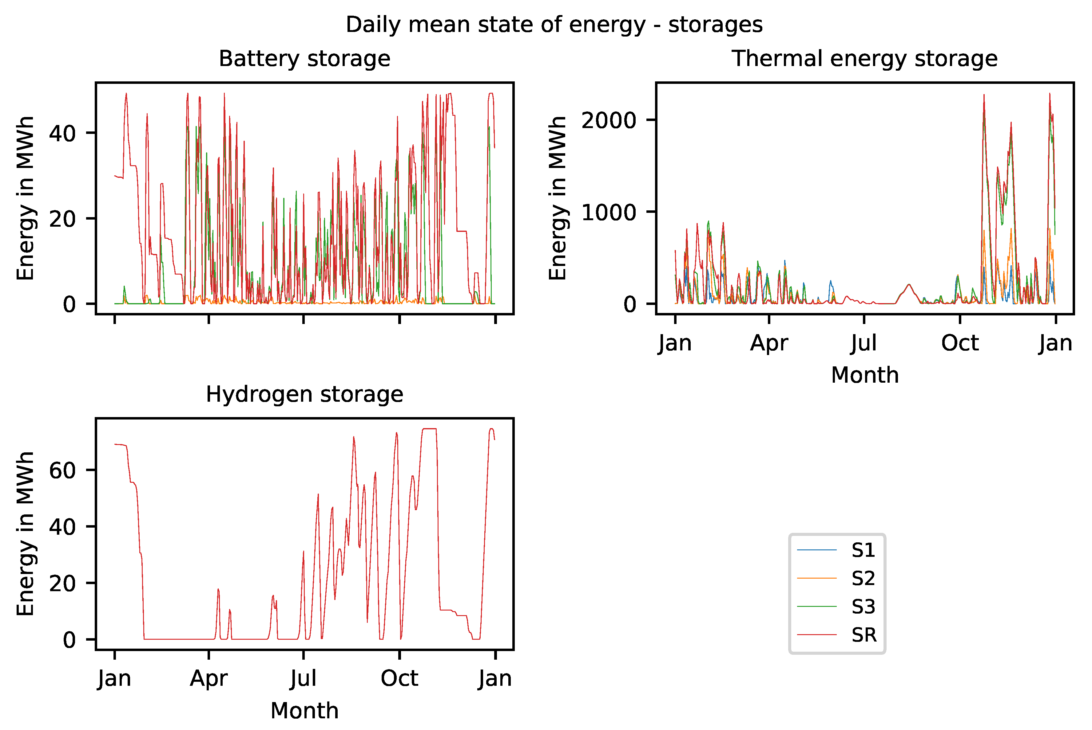
The storage facilities are operated exergy-efficiently to bridge the gap between variable RES production and demand. Figure 9 shows the daily mean state of energy. With the help of the discrete Fourier transform (DFT), the state of energies time series can be decomposed into their individual periodical components. The results in Figure 10 show the amplitude and the numbers of cycles per year. Components which are smaller than 15% of the maximum amplitude are removed from the plots.

In all four scenarios, the battery shows the highest states of energy during spring and autumn. During summer, the storage cycles are shorter, but the mean states of energy are also lower (Figure 9). The DFT analysis shows clearly defined annual (one cycle per year) and daily cycles (365 cycles per year) in all three scenarios in which a battery is installed. The thermal energy storage is mainly used during the heating season with similar peak states of energy in the beginning and the end of the year. Exceptions are S3 and SR, where the peaks in autumn are more than twice as high compared to the spring. In all four scenarios, the amplitude of annual cycle is clearly dominant. The amplitude of this annual cycle is all the more significant with larger installed storage capacities. The hydrogen storage starts to get charged in July to shift electricity from the sunny periods to autumn and winter. Its state of energy has significant annual and biannual cycles.

The full cycles that a storage can achieve depends on load and production time series, as well as the size and purpose of a storage (

Table 10. Full storage cycles per year.

	S1	S2	S3	SR
Battery storage	-	140.1	68.6	67.2
Thermal energy storage	37.7	22.2	11.5	10.3
Hydrogen storage	-	-	-	8.4

). The battery in S2 has more than twice as many full cycles compared to the ones in S3 and SR. The thermal storage has the most utilisation during the heating season and is barely utilised in summer. Although the thermal storage peak states of energies are in the same order of magnitude for spring and autumn in S1 and S2, they are more than twice as high in autumn for scenarios S3 and SR. Excess electricity is used by heat pumps to shift the excess energy from PV over longer periods to times with higher demand and less supply. This requires higher storage capacities where large shares of the total capacity are not very often used. This and the great demand difference between summer and winter leads to significantly less storage cycles compared to the battery. Even though the hydrogen storage is a seasonal storage technology, it has 8.4 full storage cycles per year.

4.2.2. Energy Imports, Excess Energy and Loads

Figure 11 shows annual energy and exergy loads, excesses, imports and the RES production. Loads, waste heat imports, biomass imports and electricity production from wind stay constant in all four scenarios. Imported electricity and natural gas, PV production and excess energy vary across scenarios with the CExC-factor for imported electricity. The higher the CExC-factor, the higher are PV-production and excess electricity, and the lower are the electricity imports. In scenario SR where the CExC-factor is the highest, no electricity is imported, but natural gas. Also, it is clearly visible that the exergy content of domestic heat is low when comparing annual energy and exergy loads of the domestic heat.

Figure 12 shows the daily mean power for loads, electricity excess, and energy imports. Electricity and process heat loads mainly fluctuate over days and weeks, the annual variations are secondary. For the domestic heat load it is different. Its major annual fluctuation is caused by its strong temperature dependency. Biomass and gas imports are the highest when the heat load is highest as well. The waste heat is consumed to its maximum extent, except for short periods in summer.

Daily average values for electricity imported from the grid show a high variability. Although there are days with very little to no consumption, those days can be followed by peaks up to an average of 12 $\mathrm{M}$$\mathrm{W}$. The highest daily average values for electricity drawn from the grid occur during the winter months. In the summer months, those peaks drop to half of those values for S1 (Figure 12). This spread increases with increasing electricity CExC-factor until no electricity is consumed in SR. Excess electricity is produced between March and November, and in winter in case of high wind production. For SR Figure 12 shows that the exported electricity decreases from its peak in spring until autumn.

4.2.3. Result Discussion

Compared to imported energy, RES can provide energy for lower expenditures, but their fluctuating production does not necessarily meet the current demand. This gap must be compensated by energy drawn from the grid, or additional local power plants and storage facilities. Between the two options, the choice depends on unit expenditures for energy imports, and the investment as well as operational expenditures for conversion units and storage facilities. The unit expenditures of the imported energy carriers limit the maximum unit expenditures of local energy production, as long as there is no import capacity restriction. The local unit expenditures for an energy carrier include expenditures for conversion units and storages, and for exergy destruction and losses. The results reflect this context in higher total expenditures and a shift from operating to infrastructure expenditures in scenarios with higher CExC factors for imported electricity. Therefore, of all the scenarios, SR has the highest installed capacities of RES and conversion units (Figure 6), and is the only one where a long-term hydrogen storage makes sense (Figure 8).

In our model, electricity imports can be seen as unrestricted, because the maximum load is well below the maximum grid capacity (Table 1 and Table 3) This means that local production is only preferred if it has lower expenditures than the energy imports. In the case of excess electricity from RES, it can be stored locally for later use or it can be returned to the grid. For a useful storage investment, unit expenditures for electricity from RES and the battery must be lower than for imported electricity. The yield for electricity export must be also considered. This is the context that leads to the installed capacities of RES and storages. In all four scenarios, the wind power potential is used to its maximum. No PV is used in S1, but it rises up to 24.8 $\mathrm{G}$$\mathrm{W}$ in SR, which is equal to 99.1% of the available potential. The higher CExC-factors for imported electricity make PV installations and battery storage practical in S2, S3 and SR. Long term storage using power to gas is exergetically only reasonable in SR.

For domestic heat, the situation is different. The maximum waste heat import power of 3 $\mathrm{M}$$\mathrm{W}$ covers only 8% of the maximum domestic heat load. The remaining heat will be provided by the plants with the lowest total unit expenditures, under the consideration that the local biomass has to be used. The biomass is used in a biomass CHP which is mainly operated in times where the heat demand is high and PV yields are low. Heat pumps together with thermal energy storage cover the rest.

From S2 to S3 the CExC-factor and therefore the unit expenditures for electricity imports rises from 1.5$\frac{\mathrm{MW}}{\mathrm{MW}}$ to 2 $\frac{\mathrm{MW}}{\mathrm{MW}}$. This results in an increase of the battery storage capacity from 2 MW h to 39.5 MW h and of the thermal energy storage from 895MW h to 2193 MW h. Apart from the two scenarios, there are no others where the increase in storage capacity is so large. As already discussed above, raising the limiting unit expenditures for electricity imports allows for higher total unit expenditures. The increase can be totally attributed to the infrastructure expenditures, because the operational unit expenditures stay constant. This tolerates lower capacity factors or annual storage cycles. Due to the fact that the investment unit expenditures follow a reciprocal function (see Figure 2), such a vast increase of the storage capacities between these two scenarios is possible.

5. Conclusions

The method of the CExC minimisation has proved to be applicable to energy systems planning and operation. The usage of CExC-factors makes the methodology applicable to a wide range of modelling tools. Aggregation concepts like the “cellular approach” [40] allow for the deployment on different spatial scales with different levels of accuracy. Even though we presented a greenfield design approach, it is also well suited for brownfield design approaches, for unit commitment, and even for optimal power flow calculations.

The major point of the overall results is that a well linked electricity and heat sector, using heat pumps and thermal energy storage, can enable a resource efficient supply while providing the necessary flexibility for integrating variable RES at the same time. Co-generation of heat and electricity is beneficial to separate production. The second point is the consideration of the load collective of the different plants. Although the operational efficiency of one technology might be higher compared to another, its high investment CExC makes this technology more costly in cases with low annual capacity factors.

In general, for the same rated power an exergy efficient plant will be larger compared to a less exergy efficient one (e.g., compare the sizes of compression and absorption chillers.) [61]. This is because exergy efficient plants have to operate with lower driving potentials, which leads to larger plants and therefore to higher CExC for the plant investment. For example, for the same heat transfer capacity, heat exchangers with higher temperature differences between the hot and the cold fluid need smaller exchange surfaces than heat exchangers with lower temperature differences. This means that operational expenditures shift to investment expenditures. Therefore, exergy efficient plants need higher capacity factors than less exergy efficient plants to reach the same unit expenditures. The variability of RES requires additional storages and dispatchable back-up plants with high capacities. This will lead to low annual capacity factors for the individual plants, which contradicts the use of exergy efficient technologies. In such cases, investment expenditures might not be negligible any more compared to the operational expenses. The CExC methodology takes both discrepancies into account and supports finding an optimal solution.

Although exergy factors for energy streams can be unambiguously calculated by thermodynamic laws, we know that the CExC-factors for the inflows do not have such a high degree of accuracy and are subject to uncertainties. The influence of the investment CExC should also not be overestimated, because in none of the scenarios it exceeds 10% (

Table 11. Share of investment and conversion losses on the total CExC input.

	S1	S2	S3	SR
	%	%	%	%
Investment	$2.1$	$4.6$	$8.0$	$9.4$
Conversion losses	$25.1$	$24.7$	$23.4$	$21.8$

). For a comparison, the conversion losses (exergy losses and destruction within the energy system) range from 21.8% to 25.1%. A sensitivity analysis of the investment CExC of the individual plant can help to get a better understanding of their implications.

Most of the current applications of technical exergy analyses differ in two points: the assessment of consumed energy carriers and materials according their physical exergy or CExC, and the use of either an energy-based or power-based perspective. Energy-based means that only the energy consumption over a certain period of time (usually one year) is considered for analysis. A power-based perspective also takes into account the variation in energy consumption over time [11].

Both of the above-stated points can have significant impacts on the relevance of the results. The use of physical exergy as an evaluation criterion could favour energy sources with high exergy losses outside the system boundaries over those produced internally. A power-based approach, as we use it in our work, is important for the sizing of system components and, in the case of involved storages, for considering their operational impact. Applications using physical exergy and a power-based approach mainly concern individual industrial processes or plants to identify internal exergy destruction and losses [5]. Energy-based perspectives are used above all when larger energy systems, in which the individual processes are no longer comprehensible, are considered over a longer period of time. Some consider only the flows of energy carriers, others include both energy and material flows [30].

Municipal energy systems lie between these two extremes. Our approach with using CExC-minimisation for design and operation of such energy systems helps to overcome this gap. It contributes to the identification of the location and magnitude of high exergy destruction and losses within the system. However, the use of CExC shows whether these are better treated within or outside the system boundaries. Including the materials for the plant investment permits optimum sizing of the plants for the respective load collective.

In future modelling applications, there are several improvements that can be made:

• A better representation of the electric grid connection. In this paper, we use a constant CExC-factor for electricity from the grid. We assume grid availability for feed in and drawing energy all the time. This might not be true for future applications. The CExC-factor might vary over the day and the seasons. There might also be shortages or congestion in the transmission grid.
• The spatial dimension. The current model does not account for the distribution of energy. Restricted energy transport capacities and the unavailability of network coverage in some areas, especially heat and gas grids, will lead to different results. The network restrictions can be modelled using total transfer capacities, or if more detail is necessary, power flow models.
• Include further technologies. Currently, only a basic set of conversion technologies (Table 4), RES (Table 6), and storages (Table 5) is used in the model. Possible additional technologies are demand side management; absorption heat pumps; solid oxide fuel; and electrolysis cells, pumped hydro, tidal energy, etc. The use of storage capacities inherited in heat and gas networks can also support the integration of RES.
• Include additional sectors. Currently, only the residential sector, and commercials, private and public services sector are considered in the model. Together they consume 34.3% of Austria’s final energy demand. The other large consumers are the industry sector with 29.3% and the transport sector with 34.4%. An incorporation of both sectors into a municipal energy system model can support in finding an exergy efficient design. A better model of industrial processes can lead to synergies between industrial and municipal energy systems. In addition, a shift to electric mobility will increase electricity demand and include a high DSM potential.

References

1. Geyer, R.; Knöttner, S.; Diendorfer, C.; Drexler-Schmid, G. IndustRiES: Energieinfrastruktur für 100% Erneuerbare Energie in der Industrie; Klima- und Energiefonds der österreichischen Bundesregierung: Wien, Austria, 2019. [Google Scholar]
2. Sejkora, C.; Kienberger, T. Dekarbonisierung der Industrie mithilfe elektrischer Energie? In Proceedings of the 15th Symposium Energieinnovation, Graz, Austria, 14–16 February 2018; Technische Universität Graz, Ed.; Technische Universität Graz: Graz, Austria, 2018. [Google Scholar]
3. Wall, G. Exergy: A Useful Concept. Ph.D. Thesis, Chalmers Tekniska Högskola. N.S, Göteborg, Sweden, 1986. [Google Scholar]
4. Wall, G. Exergy tools. Proc. Inst. Mech. Eng. Part A J. Power Energy 2003, 217, 125–136. [Google Scholar] [CrossRef]
5. Dewulf, J.; van Langenhove, H.; Muys, B.; Bruers, S.; Bakshi, B.R.; Grubb, G.F.; Paulus, D.M.; Sciubba, E. Exergy: Its Potential and Limitations in Environmental Science and Technology. Environ. Sci. Technol. 2008, 42, 2221–2232. [Google Scholar] [CrossRef] [PubMed]
6. Statistik Austria (Ed.) Nutzenergieanalyse (NEA) 2017; Statistik Austria: Wien, Austria, 2017. [Google Scholar]
7. Haas, R.; Panzer, C.; Resch, G.; Ragwitz, M.; Reece, G.; Held, A. A historical review of promotion strategies for electricity from renewable energy sources in EU countries. Renew. Sustain. Energy Rev. 2011, 15, 1003–1034. [Google Scholar] [CrossRef]
8. International Energy Agency. Key World Energy Statistics; Also Available on Smartphones and Tablets; International Energy Agency: Paris, France, 2017. [Google Scholar]
9. Kåberger, T. Progress of renewable electricity replacing fossil fuels. Glob. Energy Interconnect. 2018, 1, 48–52. [Google Scholar] [CrossRef]
10. Mancarella, P. MES (multi-energy systems): An overview of concepts and evaluation models. Energy 2014, 65, 1–17. [Google Scholar] [CrossRef]
11. Kriechbaum, L.; Scheiber, G.; Kienberger, T. Grid-based multi-energy systems—Modelling, assessment, open source modelling frameworks and challenges. Energy Sustain. Soc. 2018, 8, 244. [Google Scholar] [CrossRef] [Green Version]
12. Böckl, B.; Greiml, M.; Leitner, L.; Pichler, P.; Kriechbaum, L.; Kienberger, T. HyFlow—A Hybrid Load Flow-Modelling Framework to Evaluate the Effects of Energy Storage and Sector Coupling on the Electrical Load Flows. Energies 2019, 12, 956. [Google Scholar] [CrossRef] [Green Version]
13. Pfenninger, S.; Hawkes, A.; Keirstead, J. Energy systems modeling for twenty-first century energy challenges. Renew. Sustain. Energy Rev. 2014, 33, 74–86. [Google Scholar] [CrossRef]
14. Szargut, J.; Morris, D.R. Cumulative exergy consumption and cumulative degree of perfection of chemical processes. Int. J. Energy Res. 1987, 11, 245–261. [Google Scholar] [CrossRef]
15. Rant, Z. Exergie—Ein neues Wort für die Technische Arbeitsfähigkeit. Forsch. Auf Dem Geb. Ingenieurwesens 22 1956, 22, 36–37. [Google Scholar]
16. Krause, T.; Kienzle, F.; Art, S.; Andersson, G. Maximizing exergy efficiency in multi-carrier energy systems. In Proceedings of the Energy Society General Meeting, Providence, RI, USA, 25–29 July 2010; pp. 1–8. [Google Scholar] [CrossRef]
17. Tsatsaronis, G. Definitions and nomenclature in exergy analysis and exergoeconomics. Energy 2007, 32, 249–253. [Google Scholar] [CrossRef]
18. Valero, A.; Lozano, M.A.; Munoz, M. A general theory of exergy saving: I. On the exergetic cost. In Computer-Aided Engineering of Energy Systems: Vol 3. Second Law Analysis and Modelling, Proceedings of the Winter Annual Meeting of the American Society Mechan. Engin., Anaheim, California, 7–12 December 1986; Gaggioli, R.A., Ed.; ASME: New York, NY, USA, 1986. [Google Scholar]
19. Lozano, M.A.; Valero, A. Theory of the exergetic cost. Energy 1993, 18, 939–960. [Google Scholar] [CrossRef]
20. Tsatsaronis, G. Thermoeconomic analysis and optimization of energy systems. Prog. Energy Combust. Sci. 1993, 19, 227–257. [Google Scholar] [CrossRef]
21. Sciubba, E. Beyond thermoeconomics? The concept of Extended Exergy Accounting and its application to the analysis and design of thermal systems. Exergy Int. J. 2001, 1, 68–84. [Google Scholar] [CrossRef]
22. Szargut, J. Towards a rational evaluation of steam prices. Gospod. Cieptaa 1957, 5, 104–106. [Google Scholar]
23. Sciubba, E. Exergy-based ecological indicators: From Thermo-Economics to cumulative exergy consumption to Thermo-Ecological Cost and Extended Exergy Accounting. Energy 2019, 168, 462–476. [Google Scholar] [CrossRef]
24. Ziębik, A.; Gładysz, P. Analysis of the cumulative exergy consumption of an integrated oxy-fuel combustion power plant. Arch. Thermodyn. 2013, 34, 105–122. [Google Scholar] [CrossRef]
25. Wang, S.; Liu, C.; Liu, L.; Xu, X.; Zhang, C. Ecological cumulative exergy consumption analysis of organic Rankine cycle for waste heat power generation. J. Clean. Prod. 2019, 218, 543–554. [Google Scholar] [CrossRef]
26. Valero, A.; Lozano, M.A.; Serra, L.; Torres, C. Application of the exergetic cost theory to the CGAM problem. Energy 1994, 19, 365–381. [Google Scholar] [CrossRef]
27. Valero, A.; Lozano, M.A.; Serra, L.; Tsatsaronis, G.; Pisa, J.; Frangopoulos, C.; von Spakovsky, M.R. CGAM problem: Definition and conventional solution. Energy 1994, 19, 279–286. [Google Scholar] [CrossRef]
28. Lozano, M.A.; Valero, A. Application of the exergetic costs theory to a steam boiler in a thermal generating station. In Analysis and Design of Advanced Energy Systems: Applications, Proceedings of the Winter Meeting of the American Society of Mechanical Engineers, Boston, MA, USA, 13–18 December 1987; Moran, M.J., Stecco, S.S., Reistad, G.M., Eds.; American Society of Mechanical Engineers. Winter Annual Meeting. American Society of Mechanical Engineers. Advanced Energy Systems Division. AES (Series); ASME: New York, NY, USA, 1987. [Google Scholar]
29. Misra, R.D.; Sahoo, P.K.; Gupta, A. Application of the exergetic cost theory to the LiBr/H2O vapour absorption system. Energy 2002, 27, 1009–1025. [Google Scholar] [CrossRef]
30. Ertesvåg, I.S. Society exergy analysis: A comparison of different societies. Energy 2001, 26, 253–270. [Google Scholar] [CrossRef]
31. Ukidwe, N.U.; Bakshi, B.R. Industrial and ecological cumulative exergy consumption of the United States via the 1997 input–output benchmark model. Energy 2007, 32, 1560–1592. [Google Scholar] [CrossRef]
32. Sun, B.; Nie, Z.; Gao, F. Cumulative exergy consumption (CExC) analysis of energy carriers in China. Int. J. Exergy 2014, 15, 196. [Google Scholar] [CrossRef]
33. Causone, F.; Sangalli, A.; Pagliano, L.; Carlucci, S. An Exergy Analysis for Milano Smart City. Energy Procedia 2017, 111, 867–876. [Google Scholar] [CrossRef] [Green Version]
34. Torío, H.; Schmidt, D. Development of system concepts for improving the performance of a waste heat district heating network with exergy analysis. Energy Build. 2010, 42, 1601–1609. [Google Scholar] [CrossRef]
35. Li, H.; Svendsen, S. Energy and exergy analysis of low temperature district heating network. Energy 2012, 45, 237–246. [Google Scholar] [CrossRef]
36. Bösch, M.E.; Hellweg, S.; Huijbregts, M.A.J.; Frischknecht, R. Applying cumulative exergy demand (CExD) indicators to the ecoinvent database. Int. J. Life Cycle Assess. 2007, 12, 181–190. [Google Scholar] [CrossRef]
37. Hilpert, S.; Kaldemeyer, C.; Krien, U.; Günther, S.; Wingenbach, C.; Plessmann, G. The Open Energy Modelling Framework (oemof)—A new approach to facilitate open science in energy system modelling. Energy Strategy Rev. 2018, 22, 16–25. [Google Scholar] [CrossRef] [Green Version]
38. Oemof Developer Group. Oemof—Open Energy Modelling Framework (v0.2.2); Oemof Developer Group: Berlin, Germany, 2018. [Google Scholar] [CrossRef]
39. United Nations (Ed.) International Recommendations for Energy Statistics (IRES); Statistical Paper Series M; United Nations: New York, NY, USA, 2017. [Google Scholar]
40. Böckl, B.; Kriechbaum, L.; Kienberger, T. Analysemethode für kommunale Energiesysteme unter Anwendung des zellularen Ansatzes. In Symposium Energieinnovation; Institut für Elektrizitätswirtschaft und Energieinnovation, Ed.; TU Graz: Graz, Austria, 2016. [Google Scholar]
41. Kleinertz, B.; Pellinger, C.; von Roon, S.; Hübner, T.; Kaestle, G. EU Displacement Mix: A Simplified Marginal Method to Determine Environmental Factors for Technologies Coupling Heat and Power in the European Union; Forschungstelle für Energiewirtschaft eV: Munich, Germany, 2018. [Google Scholar]
42. Frischknecht, R.; Stucki, M.; Flury, K.; Itten, R.; Tuchschmid, M. Primärenergiefaktoren von Energiesystemen: Version 2.2; ESU-Services Ltd.: Uster, Switzerland, 2012. [Google Scholar]
43. Oemof Developer Group. The Oemof Demandlib (Oemof. Demandlib); Oemof Developer Group: Berlin, Germany, 2016. [Google Scholar] [CrossRef]
44. Pfenninger, S.; Staffell, I. Long-term patterns of European PV output using 30 years of validated hourly reanalysis and satellite data. Energy 2016, 114, 1251–1265. [Google Scholar] [CrossRef] [Green Version]
45. Staffell, I.; Pfenninger, S. Using bias-corrected reanalysis to simulate current and future wind power output. Energy 2016, 114, 1224–1239. [Google Scholar] [CrossRef] [Green Version]
46. Hellwig, M. Entwicklung und Anwendung parametrisierter Standard-Lastprofile. Ph.D. Thesis, Technische Universität München, München, Germany, 2003. [Google Scholar]
47. BDEW/VKU/GEODE. BDEW/VKU/GEODE—Leitfaden: Abwicklung von Standardlastprofilen Gas; BDEW/VKU/GEODE: Berlin, Germany, 2015. [Google Scholar]
48. E-Control. Sonstige Marktregeln Strom; Kapitel 6—Zählwerte, Datenformate und standardisierte Lastprofile; E-Control: Wien, Austria, 2012. [Google Scholar]
49. Probas. Holz-EU-KUP-Pellet-Heizung-50 kW-2030. Available online: https://www.probas.umweltbundesamt.de/php/prozessdetails.php?id=%7B4D4E8B6D-1FEC-45E5-B927-7977C6455186%7D (accessed on 17 October 2019).
50. Probas. Gas-Heizung-Brennwert-DE-2030. Available online: https://www.probas.umweltbundesamt.de/php/prozessdetails.php?id=%7BE949C50B-659D-42C4-A779-2FCCD9CCA9AF%7D (accessed on 17 October 2019).
51. Probas. el.heat pump-mono-CZ. Available online: https://www.probas.umweltbundesamt.de/php/prozessdetails.php?id=%7BCC0E4B28-80DA-11D4-9E81-0080C8426C9A%7D (accessed on 17 October 2019).
52. Ausfelder, F.; Dura, H.E. (Eds.) Optionen für ein nachhaltiges Energiesystem mit Power-to-X Technologien: Herausforderungen—Potenziale—Methoden—Auswirkungen: 1. Roadmap des Kopernikus-Projektes "Power-to-X": Flexible Nutzung erneuerbarer Ressourcen (P2X): Erstellt im Rahmen der Roadmapping-Aktivitäten im Koperinkus-Projekt "Power-to-X": Flexible Nutzung erneuerbarer Ressourcen (P2X) gefördert durch das Bundesministerium für Bildung und Technologie, 1st ed.; DECHEMA Gesellschaft für Chemische Technik und Biotechnologie e.V: Frankfurt am Main, Germany, 31 August 2018. [Google Scholar]
53. Probas. el.heating-CZ. Available online: https://www.probas.umweltbundesamt.de/php/prozessdetails.php?id=%7BCC0E4B29-80DA-11D4-9E81-0080C8426C9A%7D (accessed on 17 October 2019).
54. Probas. Holz-HS-Waldholz-HKW-DM-DE-2005/brutto. Available online: https://www.probas.umweltbundesamt.de/php/prozessdetails.php?id=%7B67221E5B-47FF-45D8-B8E2-08DF837417C3%7D (accessed on 17 October 2019).
55. Probas. Gas-BHKW-250-DE-2010/en. Available online: https://www.probas.umweltbundesamt.de/php/prozessdetails.php?id=%7B4C6CB40B-4922-4648-9922-31CE39A826C0%7D (accessed on 17 October 2019).
56. Peters, J.F.; Baumann, M.; Zimmermann, B.; Braun, J.; Weil, M. The environmental impact of Li-Ion batteries and the role of key parameters—A review. Renew. Sustain. Energy Rev. 2017, 67, 491–506. [Google Scholar] [CrossRef]
57. Heizungsdiscount24.de. 10000 Liter TWL Puffer, Pufferspeicher Typ P10000. Available online: https://www.heizungsdiscount24.de/speichertechnik/10000-liter-twl-puffer-pufferspeicher-typ-p10000.html (accessed on 17 October 2019).
58. Deutz, S.; Bongartz, D.; Heuser, B.; Kätelhön, A.; Schulze Langenhorst, L.; Omari, A.; Walters, M.; Klankermayer, J.; Leitner, W.; Mitsos, A.; et al. Cleaner production of cleaner fuels: Wind-to-wheel—environmental assessment of CO2—based oxymethylene ether as a drop-in fuel. Energy Environ. Sci. 2018, 11, 331–343. [Google Scholar] [CrossRef] [Green Version]
59. Probas. Solar-PV-multi-Rahmen-mit-Rack-DE-2030. Available online: https://www.probas.umweltbundesamt.de/php/prozessdetails.php?id=%7B05EC9CDC-9418-45CD-A333-A1CC3CCF7C48%7D (accessed on 17 October 2019).
60. Probas. Wind Mill-CZ. Available online: https://www.probas.umweltbundesamt.de/php/prozessdetails.php?id=%7BCC0E4E86-80DA-11D4-9E81-0080C8426C9A%7D (accessed on 17 October 2019).
61. Fratzscher, W.; Brodjanskij, V.; Michalek, K. Exergie: Theorie und Anwendung; Springer: Berlin/Heidelberg, Germany, 2013. [Google Scholar]
62. Probas. MetallStahl-mix-DE-2010. Available online: https://www.probas.umweltbundesamt.de/php/prozessdetails.php?id={F428D8DE-27A7-4FD6-850C-4C0DC39740DE} (accessed on 17 October 2019).
63. Probas. Chem-OrgPVC-mix-DE-2030. Available online: https://www.probas.umweltbundesamt.de/php/prozessdetails.php?id={C0A5A645-F236-4D6F-8B75-24DB0D899824} (accessed on 17 October 2019).
64. Probas. Steine-ErdenZement-DE-2010. Available online: https://www.probas.umweltbundesamt.de/php/prozessdetails.php?id={8BBACD2C-DA5F-43A7-B24B-0D49BA161D26} (accessed on 17 October 2019).
65. Probas. Chem-OrgHDPE-DE-2000. Available online: https://www.probas.umweltbundesamt.de/php/prozessdetails.php?id={0E0B299A-9043-11D3-B2C8-0080C8941B49} (accessed on 17 October 2019).
66. Probas. MetallAluminium-mix-DE-2030. Available online: https://www.probas.umweltbundesamt.de/php/prozessdetails.php?id={5CAE9D2B-4C86-4244-88B2-A79E09DC870B} (accessed on 17 October 2019).
67. Probas. MetallKupfer-DE-mix-2030. Available online: https://www.probas.umweltbundesamt.de/php/prozessdetails.php?id={AB07F312-569F-452A-82B5-3BF124101151} (accessed on 17 October 2019).
68. Probas. FabrikSilizium-Modul-multi-DE-2030. Available online: https://www.probas.umweltbundesamt.de/php/prozessdetails.php?id={C8A517A8-CC5B-4559-9747-E385A6E4FC39} (accessed on 17 October 2019).
Figure 1. Material, RES, energy imports, load and excess energy flows over the system boundaries in an energy systems (source: own representation).
Energies 13 00182 g001
Figure 2. Total unit expenditures for investment, pretreatment and exergy consumption. (Source: own representation).
Energies 13 00182 g002
Figure 3. Cumulative exergetic consumption (CExC) flows, equivalent periodic CExC flows and exergy flows in an energy system. (Source: own representation).
Energies 13 00182 g003
Figure 4. Two cell model with the exergy expenditure and yields. Conversion units, storages, renewable energy sources (RES) and the process heat load are located in the production cell. All domestic consumers are located in the production cell. (Source: own representation).
Energies 13 00182 g004
Figure 5. Exergy expenditures and yields of the different scenarios. Expenditures include CExC from energy sources, RES, and for RES and infrastructure investment. The yields include the exergy for the load and excess exergy. (Source: own representation).
Energies 13 00182 g005
Figure 6. Calculated optimum conversion unit capacities and the corresponding CExC (Source: own representation).
Energies 13 00182 g006
Figure 7. Daily mean power of the conversion units and RES. (Source: own representation).
Energies 13 00182 g007
Figure 8. Calculated optimum storage capacities and the corresponding CExC. (Source: own representation).
Energies 13 00182 g008
Figure 9. Daily mean states of energy. (Source: own representation).
Energies 13 00182 g009
Figure 10. Periodical components of the state of energy. (Source: own representation).
Energies 13 00182 g010
Figure 11. Energy sources and energy load, and the corresponding CExC, exergy load and excess exergy. (Source: own representation).
Energies 13 00182 g011
Figure 12. Daily mean power of the operational expenditures and yields. (Source: own representation).
Energies 13 00182 g012