Evaluation of an Offshore Wind Farm by Using Data from the Weather Station, Floating LiDAR, Mast, and MERRA

Abstract

Offshore wind energy is regarded as a key alternative to fossil fuels in many parts of the world. Its exploitation is based on the sound evaluation of wind resources. This study used data from a meteorological mast, a floating light detection and ranging (LiDAR) device, and the Modern-Era Retrospective Analysis for Research and Applications, a reanalysis data set established by the NASA Center for Climate Simulation, to evaluate wind resources of the Changhua-South Offshore Wind Farm. The average wind speeds evaluated at a height of 105 m in the studied wind farm were 7.97 and 8.02 m/s according to the data obtained from the floating LiDAR device and a mast, respectively. The full-load hours were 3320.5 and 3296.5 h per year when data from the LiDAR device and mast were used, respectively. The estimated annual energy production (AEP) with a probability of 50% (P₅₀) reached 314 GWh/y, whereas the AEPs with a probability of 75% (P₇₅) and with a probability of 90% (P₉₀) were 283 GWh/y and 255 GWh/y, respectively. The estimated AEP of P₇₅ was 90% of the AEP of P₅₀, whereas the estimated AEP of P₉₀ was 81% of the AEP of P₅₀. This difference might need to be considered when assessing the risk of financing a wind project.

1. Introduction

Wind energy is regarded as one of the most crucial renewable energy sources worldwide because of its resource potential and market maturity. The feasibility of wind energy has improved dramatically over the past few years. Thus, wind energy appears to be making excellent progress toward contributing to 1.5 °C-consistent pathways [1]. It is one of the most effective green energy solutions in the non-fossil-fuel policy of modern society. Low CO₂ emissions throughout their life-span render wind farms a highly reliable and efficient option at windy sites.

Despite its merits, wind energy can also cause certain environmental effects that must be carefully addressed. Studies have indicated that the visual and auditory perception of wind turbines increased significantly with wind turbine noise (WTN) levels. Onshore wind energy tends to cause noise and visual disturbance for residents in populated areas. This is particularly evident in Taiwan, where the population density reached 651 persons/km² in 2018 and two-thirds of the country’s total area is mountainous [2]. Offshore wind energy can largely avoid these environmental effects and is most suitable for islands with limited land area. Because of the annual northeastern monsoon that blows between China and Taiwan in winter, the Taiwan Strait is regarded as an excellent area for the exploitation of offshore wind energy [3]. The Program of National Energy Development of Taiwan also has the objective of replacing the use of fossil fuels and nuclear energy with that of offshore wind energy to mitigate global warming, local air pollution, risk associated with nuclear energy, and electricity supply tension [4].

The development of and investment in offshore wind farm are based on accurate wind resource evaluation, which requires reliable wind measurement data and appropriate methodologies for evaluation. Currently, mast and light detection and ranging (LiDAR) devices are the most commonly used methods worldwide for collecting offshore wind data [5,6,7]. LiDAR is a relatively recent addition to the technologies for measuring wind speed and can be used to spot-check a wind resource at different sites. LiDAR measures wind resources to heights exceeding 150 m above ground level, which is well beyond the reach of tilt-up towers. In settings where fixed masts are not feasible, LiDAR may be the sole realistic source available for wind measurement. LiDAR is generally used in conjunction with fixed masts. Total reliance on remotely sensed data is becoming more common as its accuracy and reliability continue to improve [8].

Reanalysis data sets have been developed since the mid-1990s to provide long-term wind data with high spatial coverage worldwide. They are created by using historical weather observations to drive a numerical weather prediction model. Reanalysis data have extensive records, and gridded data are available worldwide for every place covered by the model. Modern-Era Retrospective Analysis for Research and Applications (MERRA) reanalysis dataset is conducted by the NASA Center for Climate Simulation. It was reconstructed by assimilating different observations into a global model using the GEO-5 Atmospheric Data Assimilation System [9,10]. The MERRA reanalysis dataset was replaced by the MERRA-2 reanalysis dataset based on an upgrade version of the Goddard Earth Observing System Model, Version 5 (GEOS-5) data assimilation system. The spatial resolution of MERRA-2 data is approximately 50 km × 50 km [11]. Wind speed data obtained from MERRA-2 are often used in conjunction with observation data collected from weather stations to ensure the reliability of the assessment.

The optimization of wind farm layout involves identifying the optimal locations for wind turbines in a wind farm for maximizing the total energy output of the farm. One study used a biogeography-based approach to optimize wind farm layout by maximizing energy production and reducing the wake effect [12]. Another study used a geometric pattern-based approach to optimize wind farm layout by maximizing the total power output of a wind farm [13]. Park and Law employed a mathematical optimization scheme to efficiently optimize the locations of wind turbines for maximizing wind farm power production [14]. Because the threat of global warming necessitates that fossil fuels be replaced with renewable energy as soon as possible, maximizing wind farm power production has become a crucial topic in terms of wind farm optimization.

The wake effect caused by the matrix arrangement of offshore wind farms often leads to loss of energy production. The wake effect of a turbine can be divided into near wake and far wake effects. The near wake is the region spanning two or three diameters behind the turbine. The far wake is the region in which the focus lies on wake modeling, wake interference, turbulence modeling and topographic effects [15]. Far wake models can be categorized into kinetic wake models and turbulent diffusion models [16]. Kinematic wake models are based on self-similar velocity profile. The Larsen wake model [17], Frandsen [18] and Jensen’s wake model [19] belong to this class. Turbulent diffusion models solve the Reynolds-averaged Navier–Stokes equations by using a turbulence model for wake measurements [16].

Due to the difficulty of conducting measurement campaigns in offshore areas, the measured wind data for a targeted wind farm often pertains to only a short period. Such limited data sets cannot characterize long-term wind resources. The approach measure, correlate, predict (MCP) was developed to adjust on-site measurements to reflect long-term conditions. This approach can reduce the uncertainty in energy production estimation [8]. According to the national energy policy, the construction of an offshore wind farm with a capacity of 5.5 GW is planned within the period from 2020 to 2025 in Taiwan [20]. Currently, policy makers must investigate the feasibility of integrating multiple data sources for accurate prediction of such a farm’s annual energy production. The success of the domestic clean energy policy will depend on the productivity of the wind farms. Thus, this study considered whether the adoption of MCP and LiDAR, mast, and MERRA data are feasible for evaluating the wind resource and optimizing the wind farm layout. Compared with the aforementioned approaches, this study examined the applicability of data from multiple data sources, namely a floating LiDAR device, a meteorological mast, weather stations, and MERRA, for evaluating offshore wind resources.

This study used the Changhua-South Offshore Wind Farm in Taiwan to conduct a case study for evaluating the available offshore wind resource and optimizing the wind farm layout using multiple data sources. The study materials and methods are first explained in Section 2. The estimation of the long-term power production of a wind farm conducted using MCP and the resulting wind resource map are discussed in Section 3. Moreover, the resulting wind farm optimization based on the wind resource map and the estimated annual energy production (AEP) are discussed. Finally, the prediction of the AEP and the prediction accuracy are evaluated using estimated uncertainty.

2. Materials and Methods

This study used measured data from LiDAR, mast, and Central Weather Bureau (CWB) stations as short-term target data and MERRA data as long-term reference data to use MCP for estimating long-term power production of the target wind farm. The MCP results were used to estimate the wind resource available and AEP of the target wind farm through WindSim. The future AEP was predicted with a probability of 50%, 75%, and 90% by analyzing the probability and uncertainty. The flowchart of the present study is indicated in Figure 1.

2.1. Measurement Setup

The measurement campaigns in the present study were located in the western nearshore area of Taiwan (Figure 2). The location and environment of Changhua-South Offshore Wind Farm are indicated in

Table 1. Location and environment of Changhua-South Offshore Wind Farm [21].

Sea Name	Taiwan Strait
Centre latitude	23.949
Centre longitude	120.223
Area	8 km2
Depth range	17 m–26 m
Distance from shore	5.7 km
Distance from shore (computed from center)	8 km

. A floating LiDAR device and a meteorological mast were located in the northeast of the wind farm. The data from the offshore MERRA location 2 were also used for the wind resource evaluation.

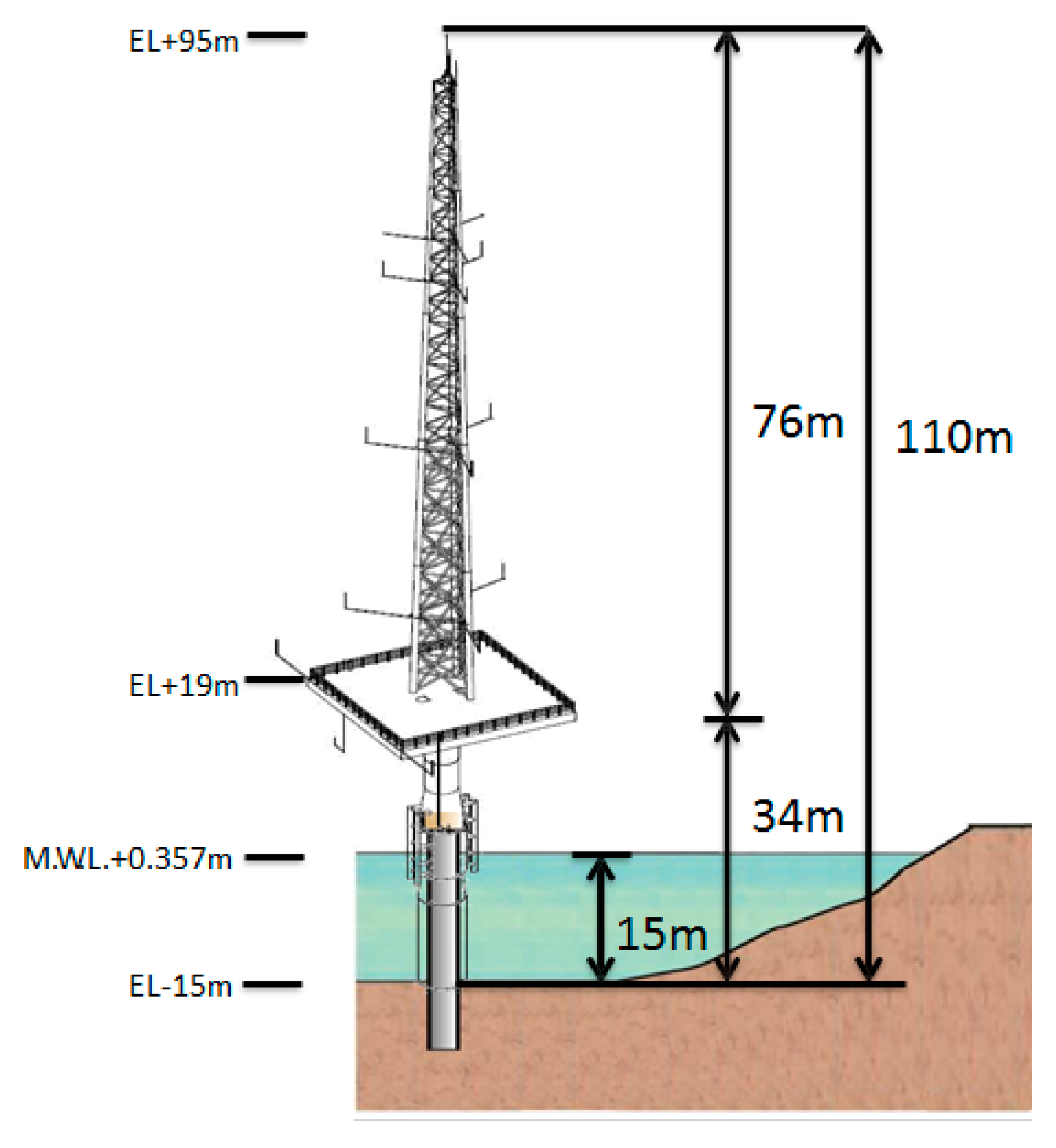
2.1.1. Meteorological Mast

The Taipower mast was located 6 km from the coastline (Figure 2), and started its measurement campaign on April 1, 2016. Two-cup anemometers and a wind vane were installed at a height of 95 m above sea level (Figure 3), and another anemometer and a wind vane were installed at a height of 50 m.

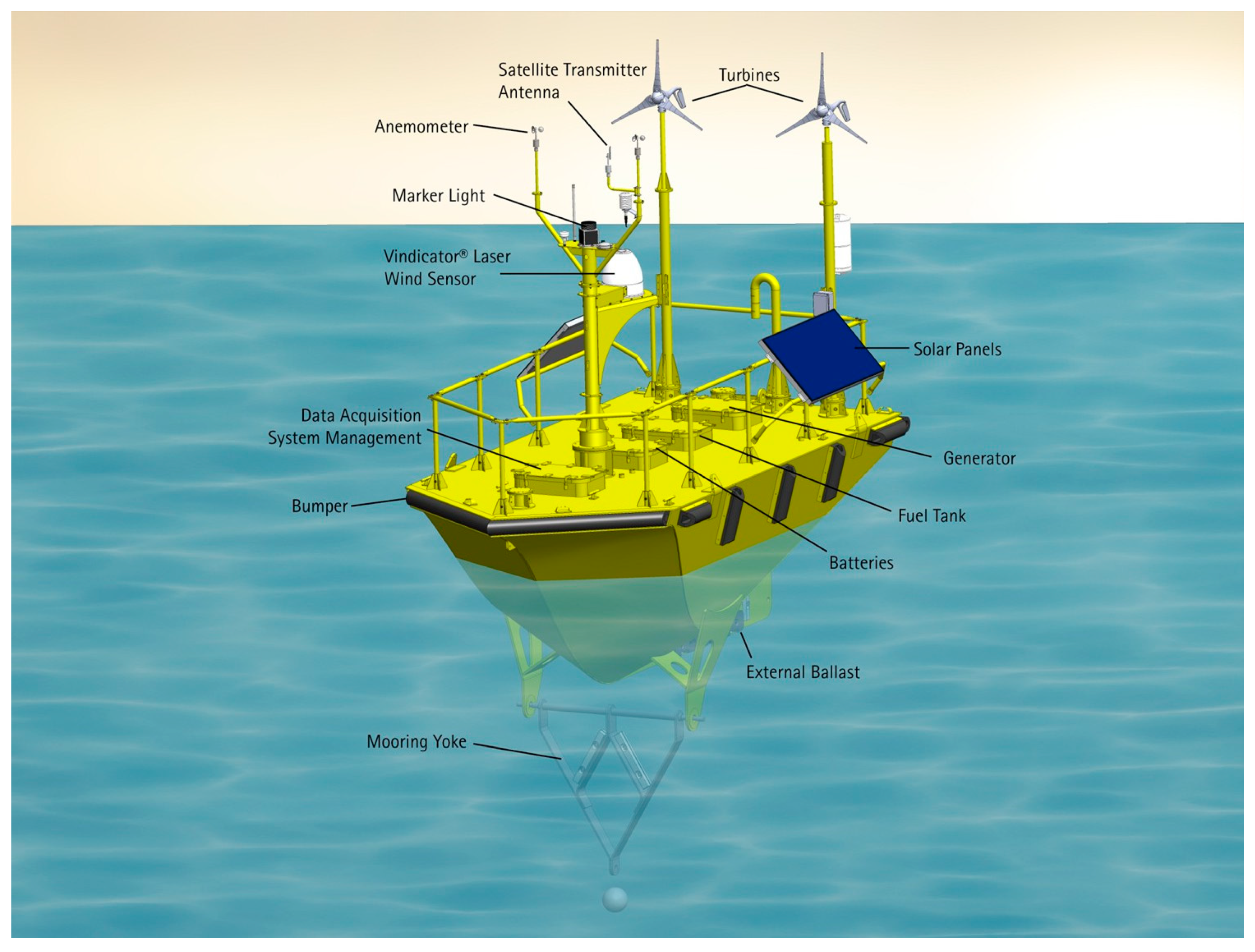
2.1.2. Floating LiDAR Device

The AXYS FLiDAR 6M floating LiDAR device used in this study was equipped with a LiDAR and a range of meteorological and oceanographic sensors, including sensors for air temperature, relative humidity, barometric pressure, surface wind, directional waves, and water temperature (Figure 4). To mitigate the effect of waves, the FLiDAR 6M uses compensation schemes for angles. The equipment consists of an anemometer, a laser wind sensor, a satellite transmitter antenna, data acquisition and data management systems, solar panels, a diesel generator, and batteries. The solar panels and diesel generator power the measurement instruments. The system was also equipped with two web cameras for security and situational awareness of the buoy. The data collected from the camera and various sensors were stored onboard the FLiDAR and transmitted in near-real time by using redundant telemetry through the onboard AXYS WatchMan 500 data management system. The FLiDAR 6M included a triple redundant power supply system that provides autonomous power throughout the year to meet the power needs of extensive sensors, telemetry, and onboard computer payload. The FLiDAR 6M uses Navy oceanographic meteorological automatic device (NOMAD) hull and mooring, which has been designed and engineered to withstand harsh weather and sea-state conditions.

The specifications of the Vindicator laser wind sensor are provided in

Table 2. Specifications for the Vindicator laser wind sensor of the FLiDAR 6M floating LiDAR device.

Specification	Value
Operating Wavelength	1550 nm
Wind Speed Range	0–90 m/s
Sensing Range	30 to 150 m
Number of Range Gates	3–6
Range Gate Depth	±20 m
Wind Speed Accuracy	±0.5 m/s
Wind Direction Accuracy	±1°
Relative Angular Accuracy	±2°
Data Output Rate	1 Hz

. The sensor can measure wind at heights ranging from 30 to 150 m. The accuracies of wind speed and wind direction are ±0.5 m/s and ±1°, respectively. The wind speed range is 0 to 90 m/s.

2.2. Datasets

Several data sources including the meteorological mast, floating LiDAR, MERRA location 2 were adopted in this study to evaluate the wind resource of the target wind farm. The data collection periods and heights for mast, MERRA (location 2), and floating LiDAR are summarized in

Table 3. Data collection periods for floating LiDAR, mast, and MERRA.

Data Source	Data Collection Period		Data Collection Heights (m)
	From	To
Floating LiDAR	22 August 2014	5 February 2015	90
Mast	1 April 2016	31 March 2017	95
MERRA	5 February 2008	4 February 2018	10, 50, 62.5

.

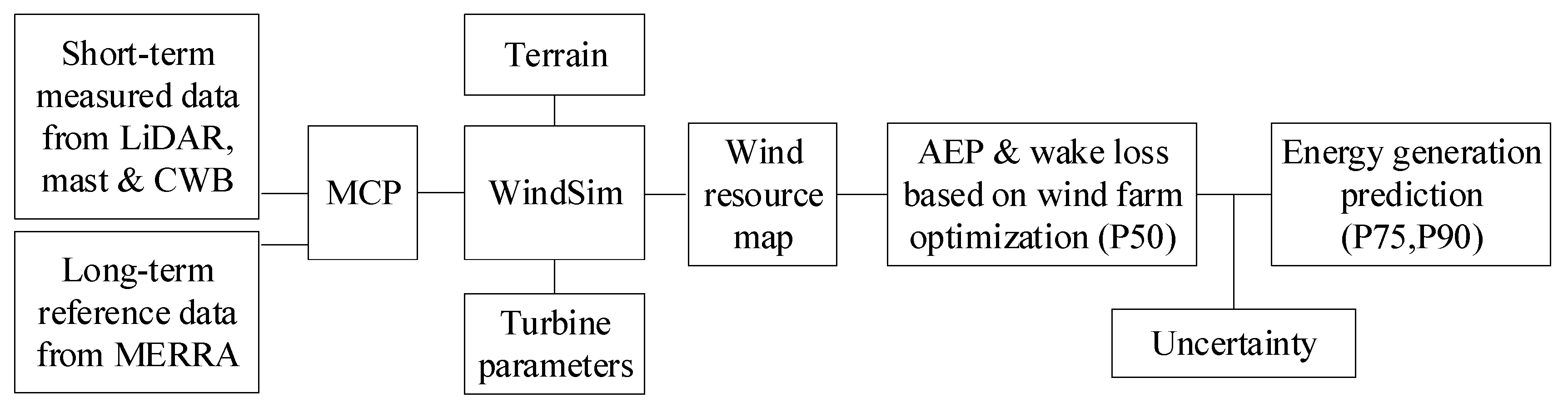
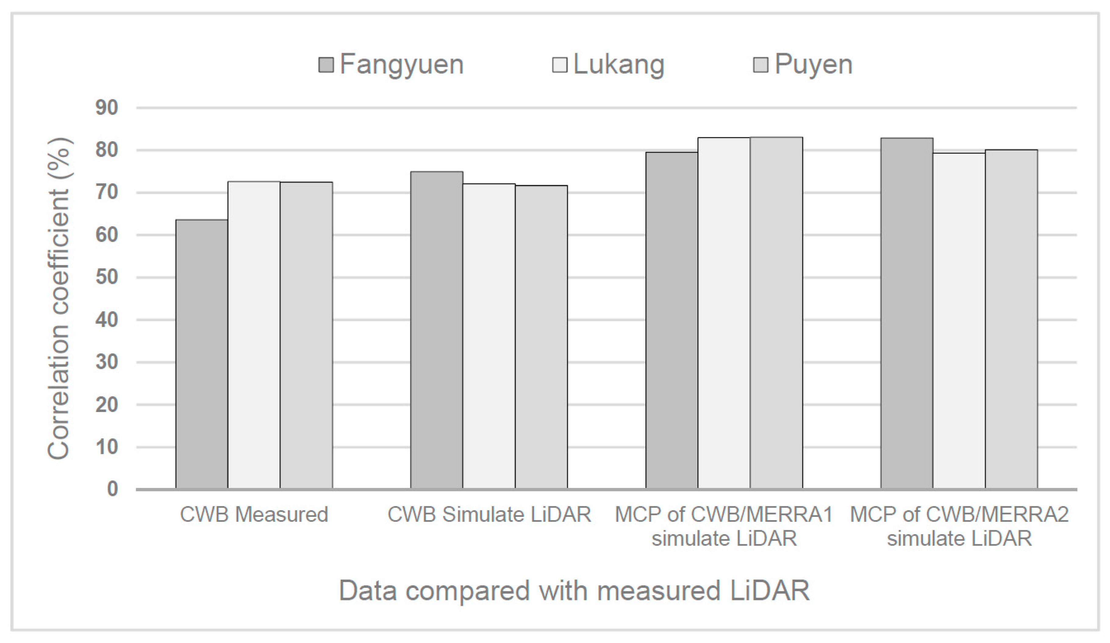
2.3. Measure-Correlate-Predict

Wind data measured for a targeted offshore wind farm often cover a few years or less. Climate adjustment is necessary for correcting measurement data collected over a limited period to make them reflective of long-term historical conditions. MCP is used to relate and adjust on-site measurements to reflect long-term conditions. The MCP method adopted in this study is based on the linear least squares (LLS) method, which is a least squares approximation of linear functions to data. The LLS MCP algorithm correlates target and reference speed data based on the linear least squares procedure to obtain a scatter plot of the target speed versus the reference speed. The resulting linear curve fit is described using slope and intercept values, that is, as the relationship presented in Equation (1).

$$y=mx+b$$

(1)

The slope and intercept for the LLS algorithm can be calculated using Equations (2) and (3).

$$m=S_{xy}/S_{xx}$$

(2)

$$b=\overline{y}-m\overline{x}$$

(3)

where $S_{xx}$ and $S_{xy}$ are given by Equations (4) and (5), respectively.

$$S_{xx}={{\displaystyle \sum }}_i{\left(x_i-\overline{x}\right)}^2,$$

(4)

$$S_{xy}={{\displaystyle \sum }}_i\left(x_i-\overline{x}\right)\left(y_i-\overline{y}\right),$$

(5)

where $x_i$ is the reference data, $\overline{x}$ is the average of the reference data, $y_i$ is the target data, and $\overline{y}$ is the average of the target data.

The MCP was validated in this study according to the following process. First, short-term data from the CWB station were used with WindSim to simulate the wind speed and wind direction of the site of floating LiDAR. The short-term target data obtained from the CWB station and long-term reference data obtained from MERRA were used to apply MCP to derive long-term data for the CWB station, which were subsequently used by WindSim to simulate the wind speed and wind direction at the site of the floating LiDAR device. The relationship between the measured data of the floating LiDAR and simulated data for the site of the floating LiDAR was then examined for validation.

MCP was conducted in this study to relate and adjust on-site measurements to a long-term reference for reducing the uncertainty in energy production estimates. The short-term data measured by the floating LiDAR device and mast were used as the target data of wind resources, and long-term data obtained from MERRA were used as reference data to conduct MCP for simulating historical wind conditions. The simulation used hourly wind speeds and wind directions. The long-term historical wind data obtained from the LiDAR device and mast were evaluated using MCP for the period between 2008 and 2018.

2.4. Wake Effect of Turbine

A comparison of wake models revealed that the Jensen far wake model achieves excellent performance for solving the wind farm layout problem because of its simplicity and relatively high accuracy [16]. The Jensen model assumes a linearly increasing wake with a velocity deficit that is based on the distance between the upstream turbine and the downstream turbine. The diameter of air at distance $x$, $D_x$, after it goes through a turbine is as follows:

$$D_x=D+2k_{d}x,$$

(6)

where $D$ is the rotor diameter and $k_d$ is the decay coefficient. For a single wake model, the downstream wind speed $U_x$ is as follows:

$$U_x=U\left[1-{\left(\frac{D}{D+2k_{d}x}\right)}^2\left(1-\sqrt{1-C_T}\right)\right],$$

(7)

where $U$ represents the upstream wind speed before it passes through a turbine and $C_T$ represents the thrust coefficient. Equation (7) can only be used in the far wake regions, where the distance should be three to five diameters for onshore and six to eight diameters for offshore regions [23]. A shadow area is observed in the wake stream of the downstream turbine (j), which is affected by the wake stream of the upstream turbine (i) [24]. Equation (7) can be rewritten as follows:

$$U_j\left(x_{ij}\right)=U_i\left[1-{\left(\frac{D}{D+2k_{d}x}\right)}^2\left(1-\sqrt{1-C_T}\right)\left(\frac{A_{shadow,i}}{A_w}\right)\right]$$

(8)

where $U_j\left(x_{ij}\right)$ represents the wind speed of the downstream turbine (j) that contains the shadow part, $U_i$ represents the wind speed after it passes through the upstream turbine (i), $A_{shadow,i}$ represents the shadow area of the wake stream, and $A_w$ represents the area of wake stream. The shadow area can be expressed as follows:

$$A_{shadow,i}={\left[r_i\left(x_{ij}\right)\right]}^2{\cos }^{-1}\left(\frac{L_{ij}}{r_i\left(x_{ij}\right)}\right)+r_0{}^2{\cos }^{-1}\left(\frac{d_{ij}-L_{ij}}{r_i\left(x_{ij}\right)}\right)-\frac{1}{2}{d}_{ij}{z}_{ij},$$

(9)

where $d_{ij}$ is the distance between two turbines measured across the wind direction, $x_{ij}$ is the distance between two turbines measured in the wind direction, $r_i\left(x_{ij}\right)$ is the radius of the wake stream, $L_{ij}$ is the distance between the upstream turbine (i) and the intersection of $A_w$ and A measured across the wind direction. Because these parameters ($x_{ij}$, $d_{ij}$, $L_{ij}$) are related to wind direction, they are adjusted as functions of wind direction as follows:

$$x_{ij}=s{p}_{ij}\cos \left({\alpha }_{ij}-dir\right),$$

(10)

$$d_{ij}=\sqrt{s{p}_{ij}{}^2-x_{ij}{}^2},$$

(11)

$$L_{ij}=\frac{d_{ij}{}^2-r_0{}^2+r_i{}^2\left(x_{ij}\right)}{2d_{ij}},$$

(12)

where $s{p}_{ij}$ is the geographic spacing between turbines i and j, $dir$ is the wind direction in degrees, and ${\alpha }_{ij}$ is the angle between the north direction (0°) and the segment linking the two turbines.

When the turbine is affected by many turbines, the velocity deficit is given as follows: [25]

$$U_j=U_0\left[1-{{\displaystyle \sum }}_{k=1}^{j-1}{\left(1-\frac{U_{kj}}{U_0}\right)}^2\right],$$

(13)

where $U_j$ represents the velocity deficit affected by multiple turbines, $U_0$ represents the upstream wind speed, and $U_{kj}$ represents the wind speed of the downstream turbine (j) that is influenced by k upstream turbines. From Equation (13), a velocity deficit occurs when air goes through the turbines, which means that the wake effect increases with an increasing number of turbines.

2.5. Annual Energy Production

AEP was calculated as follows:

$$\mathrm{AEP}=N_h{\displaystyle \sum }F\left(v\right)\times P\left(v\right),$$

(14)

where $N_h$ is the number of hours in a year, $F\left(v\right)$ is the Weibull distribution, and $P\left(v\right)$ is the power output.

2.6. WindSim Model

WindSim is a wind farm design tool and has been widely used in the wind energy industry. Its interface can be accessed using well-known software such as Global Mapper, Windographer, WindPRO, WindFarmer, and WAT [26]. For example, WindPRO defines a FLOWRES format on the basis of XML files with which the wind speed and turbulence results from WindSim can be exported into WindPRO [27]. WindSim was used in this study to optimize wind turbine placement by maximizing annual energy production while considering site and terrain constraints. It uses elevation and roughness data to build a terrain model and computational fluid dynamics to solve the following equation:

$$\rho {\overline{u}}_j\frac{\partial {\overline{u}}_j}{\partial x_j}=\rho {\overline{f}}_i+\frac{\partial }{\partial x_j}\left[-\overline{p}{\delta }_{ij}+\mu \left(\frac{\partial {\overline{u}}_i}{\partial x_j}+\frac{\partial {\overline{u}}_j}{\partial x_i}\right)-\rho \overline{u{\prime }_{i}u{\prime }_j}\right],$$

(15)

where $\rho {\overline{u}}_j\frac{\partial {\overline{u}}_j}{\partial x_j}$ represents the change in the mean momentum of the fluid element, $\rho {\overline{f}}_i$ is mean body force, $\overline{p}{\delta }_{ij}$ is isotropic stress due to the mean pressure field, $\mu \left(\frac{\partial {\overline{u}}_i}{\partial x_j}+\frac{\partial {\overline{u}}_j}{\partial x_i}\right)$ is viscous stresses, and $\rho \overline{u{\prime }_{i}u{\prime }_j}$ denotes the Reynolds stress.

The ASTER GDEM v2 Worldwide Elevation Data were used to establish elevation data for the studied area, whereas the roughness data were acquired from GlobeLand30. The parameters adopted in the study are listed in

Table 4. Parameters adopted to build a wind resource model in this study.

Properties	Categories	Parameters	Value
Terrain	Roughness	Roughness height	Read from grid gws file
Wind fields	Boundary and initial conditions	Height of boundary layer	1000 m
		Speed above boundary layer height	15 m/s
		Boundary condition at top	No-friction wall
	Physical models	Potential temperature	Disregard temperature
		Air density	1.225
		Turbulence model	Standard k-ε
	Calculation parameters	Solvers	GCV
Wind Resources	Wind resource map	Heights	105
Energy	IEC Classification *	Wind speeds range Ieff	IEC standards *

* IEC: International Electrotechnical Commission.

. Solutions converge with the general collocated velocity (GCV) method. The standard k-ε turbulence model comprises two equations.

For turbulent kinetic energy k:

$$\frac{\partial \left(\rho k\right)}{\partial t}+\frac{\partial \left(\rho k{u}_i\right)}{\partial x_i}=\frac{\partial }{\partial x_j}\left[\frac{{\mu }_t}{{\sigma }_k}\frac{\partial k}{\partial x_j}\right]+2{\mu }_t{E}_{ij}{E}_{ij}-\rho ϵ.$$

(16)

For dissipation $ϵ$:

$$\frac{\partial \left(\rho ϵ\right)}{\partial t}+\frac{\partial \left(\rho ϵu_i\right)}{\partial x_i}=\frac{\partial }{\partial x_j}\left[\frac{{\mu }_t}{{\sigma }_{ϵ}}\frac{\partial ϵ}{\partial x_j}\right]+C_{1ϵ}\frac{ϵ}{k}2{\mu }_t{E}_{ij}{E}_{ij}-C_{2ϵ}\rho \frac{{ϵ}^2}{k},$$

(17)

where $u_i$ represents the velocity component in the corresponding direction, $E_{ij}$ represents the component of rate of deformation, and ${\mu }_t$ represents eddy viscosity.

2.7. Wind Turbine

In this study, the MHI Vestas Offshore V164-9.5 MW turbine with a hub height of 107 m was selected for evaluating the potential of wind power generation.

2.8. Wind Farm Optimization

In this study, the Park Optimizer module of WindSim was applied using computational fluid dynamics (CFD) results and optimization algorithms to optimize the design of IEC-compliant wind farm layouts [28,29]. The Jenson model was used as the wake model, and the decay coefficient $k_d$ set to 0.05 for the offshore condition [30]. The module sets the limitation for turbines based on the terrain condition, inflow angle, turbulence intensity, and velocity and then determines the interturbine distance required to avoid the wake effect.

2.9. Uncertainty in Wind Resource Assessment

The results of wind resource forecasting can be affected by uncertainty due to measurements and power curves. The uncertainty for 1 year of measurement is assumed to be 4% without a reference data source or thorough data analysis [8]. Uncertainty for future wind resources is calculated as follows:

$${\sigma }_{future}=\sqrt{{\sigma }_{normal}{}^2+{\sigma }_{climate}{}^2},$$

(18)

$${\sigma }_{normal}\cong \frac{\sigma }{\sqrt{N_p}},$$

(19)

where ${\sigma }_{future}$ is an uncertainty in the future, ${\sigma }_{normal}$ represents the uncertainty of the years considered for prediction, ${\sigma }_{climate}$ is the climate change uncertainty, and N_p is the number of years used for estimating uncertainty in the future and σ is the uncertainty for 1 year. Uncertainty because of climate change is assumed to be 0.5% when N_p equals 10 years [8].

Uncertainty in long-term wind prediction is derived from the correlation coefficient of the wind speed between the target and reference sites. Correlation coefficients of >0.9, 0.9–0.8, and 0.7–0.6 indicated wind speed correlation uncertainties of <1%, 1%–2%, and 3%–5%, respectively [31]. The uncertainty in the power curve is mainly caused by turbulence, air density, and shear characteristics of the site, and its value is usually 6% [32].

For forecasting the energy production probability, parameters pertaining to uncertainty should be used. The calculation of probability is as follows:

$$P_x=P_{50}\times \left(1-z\times \sigma \right),$$

(20)

where P_x represents the energy production for probability x, z represents the value of normal distribution for a specific probability presented in

Table 5. Normal distribution of specific probabilities and their corresponding z values [33].

Probability of Exceedance (%)	z
99	2.326
95	1.645
90	1.282
85	1.036
84	1.000
80	0.842
75	0.674
50	0
25	0.674
10	1.282
1	2.326

, and σ represents the uncertainty for 1 year.

3. Results and Discussion

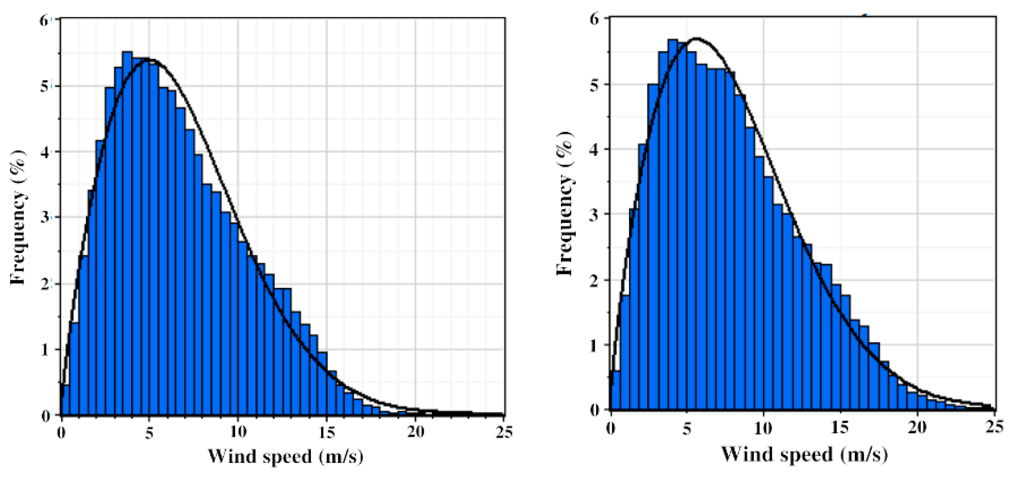
3.1. Estimating the Long-Term Power Production of a Wind Farm Using MCP

This study conducted a correlation analysis to compare floating LiDAR data that was simulated using MCP through CWB and MERRA data with measured floating LiDAR data for validating the simulation accuracy of WindSim. The information and wind measurement data of CWB stations are summarized in

Table 6. Information and wind measurement data of CWB stations [34].

Station	Measurement Height (m)	Year	Annual Average Wind Speed (m/s)	Annual Average Wind Direction (Degree)	Environment
Fangyuen	12	2016	2.5	58	Surrounded by low-rise buildings
		2017	2.5	62
		2018	2.5	40
Lukang	17	2016	3.0	49	Few buildings around, surrounded by undeveloped wetlands
		2017	2.9	27
		2018	2.6	47
Puyen	15	2016	3.3	32	Few buildings around, mostly surrounded by farmland
		2017	3.1	47
		2018	3.0	38

and Figure 5. The relationship between the simulated wind speed at the site of the floating LiDAR device and the measured wind speed obtained using the floating LiDAR device is presented in Figure 6. The correlation coefficients of the wind speed obtained using the measured floating LiDAR data and CWB station data ranged between 63.6% and 72.6%. The correlation coefficients of the measured wind speed pertaining to the measured floating LiDAR data and floating LiDAR data simulated using CWB data increased and ranged between 71.7% and 74.9%. The correlation coefficients of wind speed obtained using measured floating LiDAR data and floating LiDAR data simulated through MCP by using CWB data and MERRA data further increased and ranged between 79.7% and 83.1%. This indicates that the MCP process improved the simulation accuracy. The WindSim simulation could also be validated through these correlation analyses. The root mean square errors (RMSEs) of the wind speed obtained using the measured floating LiDAR data and floating LiDAR data simulated through MCP by using CWB data and MERRA location 1 data were smaller than the RMSE using of the wind speed obtained using the MERRA location 2 data (

Table 7. Correlation and RMSE of the wind speed for measured floating LiDAR data and floating LiDAR data simulated through MCP by using CWB data and MERRA data.

CWB Stations	MERRA Locations	R2 (%)	RMSE (m/s)
Lukang	1	83.0	4.8
	2	79.4	5.7
Puyen	1	83.1	4.4
	2	80.2	8.2

), although MERRA 1 is located farther than MERRA 2 (Figure 2).

The data from the LiDAR device and mast were processed through the MCP method by using MERRA location 2 data to produce long-term historical wind data for evaluating wind resources and predicting power generation by the Changhua-South Wind Farm. The long-term historical wind data obtained from the LiDAR device and mast for the period between 2008 and 2018 were evaluated using MCP. The data measured by the floating LiDAR device and mast represented the target data of the wind resource, and the MERRA data represented the reference data. The Weibull distribution and wind direction of the wind resource for the CWB, LiDAR device, and mast after using MCP are discussed as follows.

3.1.1. Floating LiDAR Device

The Weibull distribution of wind resources at the site of the floating LiDAR device after using MCP is illustrated in Figure 7. The values of the shape parameter (k) and scale parameter (λ) of the Weibull distribution at the site of the floating LiDAR device were 1.85 and 7.61 m/s, respectively. The wind speed averaged 7.89 m/s and was distributed mainly between 0 and 15 m/s. The wind direction was dominated by north–northeast and north winds, followed by south–southwest wind (Figure 8).

3.1.2. Mast

The Weibull distribution of wind resources at the site of the mast after using MCP is illustrated in Figure 7. The values of the shape parameter (k) and scale parameter (λ) of the Weibull distribution were 1.80 and 8.87 m/s, respectively. The wind speed averaged 7.89 m/s and was distributed mainly between 0 and 20 m/s. The wind direction was dominated by north–northeast and north winds, followed by south–southwest wind, as was the case for the LiDAR device (Figure 8).

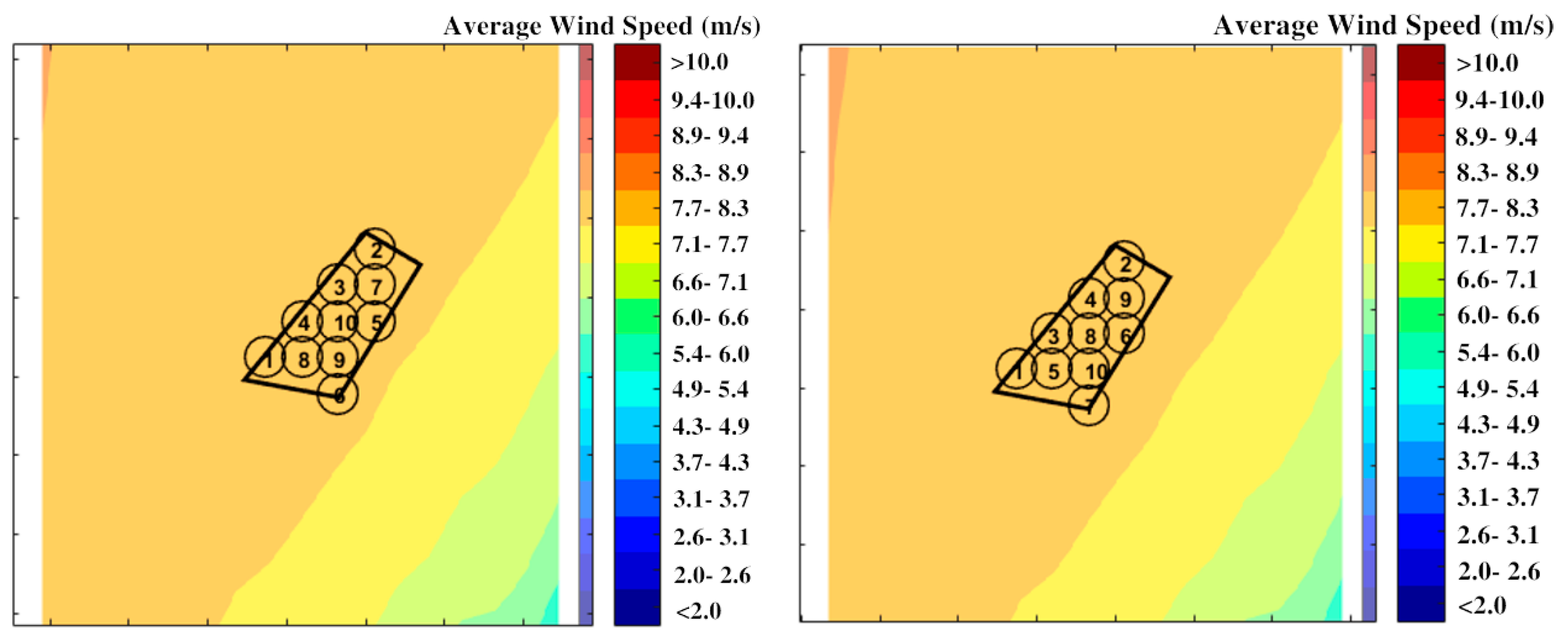
3.2. Wind Resource Map

The wind resource map was created using WindSim and MCP data derived from the floating LiDAR device and mast, as illustrated in Figure 9. The evaluated average wind speed at a height of 105 m in the studied wind farm were 7.97 and 8.02 m/s according to the data from the floating LiDAR device and mast, respectively. The amounts of offshore wind resources evaluated using data from the LiDAR device and mast were similar. The wind shear exponent at the site of the mast was estimated to be 0.05 in this study according to 10-min wind speed data measured by the mast. The vertical wind shear profile at the mast site is illustrated in Figure 10. A study indicated that the wind shear exponent onshore in Taiwan could reach between 0.18 and 0.23 [35], which is considerably higher than the value of 0.05 observed offshore.

3.3. Wind Farm Optimization

The Park Optimizer module identified the optimal locations for different numbers of turbines to maximize power generation and minimize the wake effect. The results of the optimized wind farm layouts based on the wind resource map using MCP data from the floating LiDAR device and mast were similar, as indicated in Figure 9.

3.4. Annual Energy Production

The power generation of the wind farm was estimated on the basis of the optimized wind farm layout. The results for gross AEP reached 344 GWh per year when data from the LiDAR device was used (

Table 8. Estimated power generation by the wind farm according to WindSim and MCP with data from the floating LiDAR device and MERRA. The assigned turbine numbers are the same as in Figure 9.

Turbine Number	Wind Speed (m/s)	Wind Speed Including Wake Losses (m/s)	Power Density (W/m2)	Gross AEP (MWh/y)	AEP with Wake Losses (MWh/y)	Wake Loss (%)	Full Load Hours (h/y)
1	8.03	7.98	678.0	34,522.1	34,087.2	1.26	3588.1
2	8.02	7.87	677.7	34,485.8	33,258.8	3.56	3500.9
3	8.03	7.84	677.9	34,505.1	32,936.8	4.55	3467.0
4	8.03	7.87	678.5	34,540.3	33,132.1	4.08	3487.6
5	8.00	7.55	671.9	34,302.8	30,636.5	10.69	3224.9
6	7.99	7.54	669.5	34,235.0	30,445.9	11.07	3204.8
7	8.01	7.53	675.0	34,401.0	30,362.7	11.74	3196.1
8	8.02	7.60	676.3	34,473.3	30,856.0	10.49	3248.0
9	8.00	7.48	672.7	34,341.7	29,876.6	13.00	3144.9
10	8.02	7.47	675.5	34,429.9	29,853.7	13.29	3142.5
All	-	-	-	344,237.0	315,446.3	-	-
Mean	8.02	7.67	675.3	-	-	8.36	3320.5

) and reached 342 GWh per year when using data from the mast (

Table 9. Estimated power generation of the wind farm according to WindSim and MCP with data from the mast and MERRA. The assigned turbine numbers are the same as those in Figure 9.

Turbine Number	Wind Speed (m/s)	Wind Speed Including Wake Losses (m/s)	Power Density (W/m2)	Gross AEP (MWh/y)	AEP with Wake Losses (MWh/y)	Wake Loss (%)	Full Load Hours (h/y)
1	7.99	7.94	664.3	34,294.8	33,860.7	1.27	3564.3
2	7.98	7.83	664.0	34,257.3	33,001.2	3.67	3473.8
3	7.99	7.82	664.8	34,311.0	32,879.9	4.17	3461.0
4	7.98	7.80	664.2	34,276.3	32,679.0	4.66	3439.9
5	7.98	7.56	662.6	34,245.0	30,657.9	10.47	3227.1
6	7.97	7.49	661.2	34,171.4	30,135.4	11.81	3172.1
7	7.95	7.50	655.6	34,008.5	30,246.4	11.06	3183.8
8	7.97	7.43	661.7	34,200.1	29,623.7	13.38	3118.3
9	7.96	7.51	658.0	34,071.3	30,432.0	10.68	3203.4
10	7.96	7.44	658.9	34,112.6	29,651.2	13.08	3121.2
All	-	-	-	341,948.3	313,167.4	-	-
Mean	7.97	7.63	661.5	-	-	8.42	3296.5

). The full-load hours achieved were 3320.5 and 3296.5 h per year when using data from the LiDAR device and mast, respectively. The estimated power generation of the wind farm was similar when using data from the LiDAR device and mast, although the AEP evaluated using data from the LiDAR device was higher than that from mast, probably because the LiDAR device was located more offshore than the mast was, where higher wind speed prevailed.

The estimated wake losses of wind turbines were between 1% and 14% and average wake losses were 8.36% and 8.42% when using data from the LiDAR device and mast, respectively. Because the winter northern monsoon wind constituted the prevailing wind resource, upstream turbines 1–4 northward were least affected by wake loss and exhibited losses of 1%–5%; however, downstream turbines 5–10 were most affected and exhibited 10%–13% loss.

The effects of wake loss on wind speed and AEP in various sectors can be observed in

Table 10. Effects of wake loss on wind speed and AEP in various sectors determined using data from the floating LiDAR device and mast.

Sector	Wind Speed (m/s)		AEP with Wake Losses (MWh/y)
	Floating LiDAR	Mast	Floating LiDAR	Mast
345°–15°	−0.05%	−0.05%	−0.09%	−0.09%
15°–45°	−0.02%	−0.02%	−0.03%	−0.03%
45°–75°	−0.02%	−0.02%	−0.09%	−0.08%
75°–105°	−0.02%	−0.02%	−0.19%	−0.19%
105°–135°	-0.01%	−0.01%	−0.04%	−0.04%
135°–165°	0.00%	−0.01%	−0.02%	−0.02%
165°–195°	−0.07%	−0.07%	−0.14%	−0.14%
195°–225°	−0.03%	−0.03%	−0.07%	−0.07%
225°–255°	−0.03%	−0.03%	−0.08%	−0.08%
255°–285°	−0.04%	−0.04%	−0.14%	−0.14%
285°–315°	−0.01%	−0.01%	−0.04%	−0.04%
315°–345°	−0.01%	−0.01%	−0.02%	−0.02%

. The wake loss exhibited the highest effect on wind speed in the sector 165°–195°, with a reduction of 0.07% in wind speed. The wake loss exhibited the highest effect on the AEP of the sector 75°–105°, causing a reduction of 0.19% in AEP. The east wind (75°–105°) exhibited the highest effect on AEP, followed by the west wind (255°–285°). However, the frequencies of occurrence of the east and west winds were the lowest in the Changhua offshore area (Figure 8). The effects of wake loss on the prevailing north–northeast (15°–45°) and south–southwest (195°–225°) winds were minimal and reduced the AEP by only 0.03% and 0.07%, respectively. This indicated that the optimization of the wind farm layout had been achieved. The examination of the wake loss for upstream and downstream wind turbines and for various sectors validated the optimization of the wind farm performed by the WindSim optimizer model.

3.5. Prediction of Annual Energy Production

Uncertainties were used to estimate probable AEP. The uncertainties of parameters are indicated in

Table 11. Uncertainties associated with parameters [33].

	Parameter	Uncertainty (%)
Wind resource	Measurement	2.04
	Tower effect	0.5
	Historical wind resource	4
	Future wind resource (10yrs)	1.4
	Long-term correlation	Inconstant
Energy level	Wind flow model	6
	Power curve	6
	Energy losses (wake effect)	Inconstant

. The uncertainty caused by long-term correlations was derived from the correlation coefficient of the wind speed between the target site and the reference site, whereas that caused by energy losses was based on wind farm optimization (

Table 12. Inconstant uncertainty of AEP estimation.

	Inconstant
	Long-Term Correlation (%)	Energy Losses (%)
Floating LiDAR	1.61	8.36
Mast	4.05	8.42

). The data from the LiDAR device and mast were processed through the MCP method using data obtained at MERRA location 2. The relationships between the generated MCP data and measured data from the LiDAR device and mast were analyzed. The correlation coefficients of >0.9, 0.9–0.8, and 0.7–0.6 indicated wind speed correlation uncertainties of <1%, 1%–2%, and 3%–5%, respectively [31]. The uncertainty of long-term correlation was calculated using the interpolation method (Table 12), and the energy losses caused by the wake effect were calculated using WindSim.

P₅₀ represents the assessment of power production without considering uncertainties. P₇₅ and P₉₀ can be estimated using Equations (21) and (22) derived from Equation (20). The AEP estimated using data from the floating LiDAR device was slightly higher than that estimated using data from the mast (Figure 11), probably because the LiDAR device was located more offshore than the mast, where higher wind speeds prevailed. The predicted energy production decreased with increasing probability. The estimated AEP of P₅₀ reached 314 GWh/y, whereas those of P₇₅ and P₉₀ were merely 283 GWh/y and 255 GWh/y, respectively. The estimated AEP of P₇₅ was 90% of that of P₅₀, whereas the estimated AEP of P₉₀ was 81% of that of P₅₀. This difference might need to be considered by investors when assessing the risk of financing a wind project.

$$P_{75}=P_{50}\times \left(1-0.674\times \sigma \right),$$

(21)

$$P_{90}=P_{50}\times \left(1-1.282\times \sigma \right),$$

(22)

where $P_x$ is the energy production for probability x and σ is the uncertainty for 1 year. The values of 0.674 and 1.282 in Table 5 are the z values for the probabilities of events exceeding the 25% and 10% thresholds, respectively.

4. Conclusions

This study used data from a floating LiDAR device, mast, and MERRA to evaluate the wind resources of the Changhua-South Offshore Wind Farm and optimize wind farm design. The power generation potential of the target wind farm was first estimated. The Park Optimizer module of WindSim was then used to identify turbine locations with the highest wind speeds and lowest turbulence to maximize energy production. Finally, the prediction accuracy of AEP was evaluated on the basis of estimated uncertainty. The crucial findings are as follows.

The average wind speeds evaluated at a height of 105 m in the studied wind farm using WindSim and MCP data derived from the floating LiDAR device and mast were 7.97 and 8.02 m/s, respectively. The predictions for energy production of the wind farm indicated that the AEP will become increasingly conservative with an increasing probability value. The estimated AEP of P₅₀ reached 314 GWh/y, whereas that of P₇₅ and P₉₀ was merely 283 GWh/y and 255 GWh/y, respectively. The estimated AEP of P₇₅ was 90% of that of P₅₀, whereas the estimated AEP of P₉₀ was 81% of that of P₅₀. This difference might need to be considered by investors when assessing the risk of financing a wind project.

This study offers novel contributions to the literature by examining the applicability of data from multiple sources, namely a floating LiDAR device, a meteorological mast, and MERRA, for evaluating offshore wind resources. The analysis results indicated that the use of MERRA data to conduct MCP enhances the prediction accuracy of energy production of an offshore wind farm. Mast and LiDAR data were used as the target data and MERRA data served as the reference data in MCP for predicting the offshore wind power generation.

Future research can be conducted to improve the accuracy of wind power estimation. Although hourly data are the most common source for the estimation of wind power generation, methods using such data may not be able to track changes in wind direction. The question of whether the accuracy of wind resource estimation can be enhanced by using data with a higher temporal resolution (e.g., 10-min data) merits investigation. Moreover, the energy production estimation in this study was based on the power curve and wind speed statistics. However, the gust factor and air density also affect the energy production of wind turbines. Further investigation can be undertaken to determine whether more weather data can help improve the accuracy of power generation estimation.

References

1. Intergovernmental Panel on Climate Change (IPCC). Global Warming of 1.5 °C. 2018. Available online: https://www.ipcc.ch/sr15/ (accessed on 15 July 2019).
2. National Development Council (NDC). The Statistical Yearbook of Construction and Planning 2018; National Development Council: Taipei, Taiwan, 2019. [Google Scholar]
3. 4C Offshore, Global Offshore Wind Speeds Rankings. 2018. Available online: http://www.4coffshore.com/windfarms/windspeeds.aspx (accessed on 24 April 2018).
4. Ministry of Economic Affairs. Program of National Energy Development; Ministry of Economic Affairs: Taipei, Taiwan, 2017.
5. Kim, J.-Y.; Oh, K.-Y.; Kim, M.-S.; Kim, K.-Y. Evaluation and characterization of offshore wind resources with long-term met mast data corrected by wind lidar. Renew. Energy 2019, 144, 41–55. [Google Scholar] [CrossRef]
6. Ørsted A/S. Offshore Wind Data. Ørsted A/S, 2019. Available online: https://orsted.com/en/Our-business/Offshore-wind/Wind-Data (accessed on 3 September 2019).
7. Sharma, P.K.; Warudkar, V.; Ahmed, S. Application of lidar and measure correlate predict method in offshore wind resource assessments. J. Clean. Prod. 2019, 215, 534–543. [Google Scholar] [CrossRef]
8. Brower, M. Wind Resource Assessment: A Practical Guide to Developing a Wind Project; John Wiley & Sons: New York, NY, USA, 2012. [Google Scholar]
9. Rienecker, M.M.; Suarez, M.J.; Gelaro, R.; Todling, R.; Bacmeister, J.; Liu, E.; Bosilovich, M.G.; Schubert, S.D.; Takacs, L.; Kim, G.K.; et al. MERRA: NASA’s Modern-Era Retrospective Analysis for Research and Applications. J. Clim. 2011, 24, 3624–3648. [Google Scholar] [CrossRef]
10. Ren, G.; Wan, J.; Liu, J.; Yu, D. Characterization of wind resource in China from a new perspective. Energy 2019, 167, 994–1010. [Google Scholar] [CrossRef]
11. Bosilovich, M.G.; Lucchesi, R.; Suarez, M. MERRA-2: File Specification. NASA Global Modeling and Assimilation Office, Note Number 9 (Version 1.1). 2016. Available online: http://gmao.gsfc.nasa.gov/pubs/office_notes (accessed on 16 July 2019).
12. Bansal, J.C.; Farswan, P. Wind farm layout using biogeography based optimization. Renew. Energy 2017, 107, 386–402. [Google Scholar] [CrossRef]
13. Patel, J.; Savsani, V.; Patel, V.; Patel, R. Layout optimization of a wind farm using geometric pattern-based approach. Energy Procedia 2019, 158, 940–946. [Google Scholar] [CrossRef]
14. Park, J.; Law, K.H. Layout optimization for maximizing wind farm power production using sequential convex programming. Appl. Energy 2015, 151, 320–334. [Google Scholar] [CrossRef]
15. Sanderse, B. Aerodynamics of Wind Turbine Wakes Literature Review; Energy Research Centre of Netherlands ECN-E-09-016: Sint Maartensvlotbrug, The Netherlands, 2009. [Google Scholar]
16. Shakoor, R.; Hassan, M.Y.; Raheem, A.; Wu, Y.-K. Wake effect modeling: A review of wind farm layout optimization using Jensen’s model. Renew. Sustain. Energy Rev. 2016, 58, 1048–1059. [Google Scholar] [CrossRef]
17. Larsen, G.C. A Simple Wake Calculation Procedure; Risø National Laboratory: Roskilde, Denmark, 1988. [Google Scholar]
18. Frandsen, S.T. Turbulence and Turbulence-Generated Structural Loading in Wind Turbine Clusters; Risø National Laboratory: Roskilde, Denmark, 2007. [Google Scholar]
19. Jensen, N.O. A Note on Wind Generator Interaction; Risø National Laboratory: Roskilde, Denmark, 1983. [Google Scholar]
20. Ministry of Economic Affairs. Essentials of Capacity Allocation for Offshore Wind Power Planning Sites. Ministry of Economic Affairs of Taiwan. Available online: https://www.moeaboe.gov.tw/ECW/populace/Law/Content.aspx?menu_id=2870 (accessed on 8 December 2019).
21. 4C Offshore, Global Offshore Wind Farms. 2018. Available online: https://www.4coffshore.com/windfarms/windfarms.aspx?windfarmid=TW11&windfarmid=TW11 (accessed on 24 April 2018).
22. Mes, J.C.; de Goffau, P.L. Stabilizing Control System of a Platform on a Buoy for Offshore Wind Assessment; Delft University of Technology: Delft, The Netherlands, 2014. [Google Scholar]
23. Han, T. The Assessment of Dynamic Wake Effects on Loading. Master’s Thesis, Department of Aerospace Engineering, Delft University of Technology, Delft, Netherlands, 2011. [Google Scholar]
24. Manwell, J.F.; McGowan, J.G.; Rogers, A.L. Wind Energy Explained—Theory, Design and Application; John Wiley & Sons: Chichester, UK, 2002. [Google Scholar]
25. Abbes, M.; Allagui, M. Centralized control strategy for energy maximization of large array wind turbines. Sustain. Cities Soc. 2016, 25, 82–89. [Google Scholar] [CrossRef]
26. WindSim, A.S. Introduction of WindSim Software; WindSim AS: Tønsberg, Norway, 2015. [Google Scholar]
27. Meissner, C.; Mana, M.; de Groot, T. Recent developments of WindSim. In Proceedings of the WindSim 14th User Meeting, Tønsberg, Norway, 5–6 June 2019. [Google Scholar]
28. Meissner, C.; Vogstad, K.; Welle-Strand Horn, U. Park optimization using IEC constraints for wind quality. In Proceedings of the European Wind Energy Conference, Brussels, Belgium, 14–17 March 2011. [Google Scholar]
29. Meissner, C. WindSim: Getting Started; WindSim AS: Tønsberg, Norway, 2019. [Google Scholar]
30. Hwang, C.; Jeon, J.H.; Kim, G.H.; Kim, E.; Park, M.; Yu, I.K. Modeling and simulation of the wake effect in a wind farm. J. Int. Counc. Electr. Eng. 2015, 5, 74–77. [Google Scholar] [CrossRef] [Green Version]
31. Garrad Hassan, G.L. Uncertainty Analysis. In WindFarmer Theory Manual; Garrad Hassan, G.L., Ed.; Garrad Hassan & Partners Ltd.: Bristol, UK, 2011; pp. 6–39. [Google Scholar]
32. Kwon, S.D. Uncertainty analysis of wind energy potential assessment. Appl. Energy 2010, 87, 856–865. [Google Scholar] [CrossRef]
33. Lira, A.; Rosas, P.; Araujo, A.; Castro, N. Uncertainties in the estimate of wind energy production. In Proceedings of the Energy Economics Iberian Conference, Lisbon, Portugal, 4–5 February 2016. [Google Scholar]
34. Central Weather Bureau (CWB). CWB Observation Data Inquire System. Available online: http://e-service.cwb.gov.tw/HistoryDataQuery/ (accessed on 12 December 2019).
35. Chang, P.C.; Hung, J.B.; Lin, T.H. The Analysis of Wind Characteristics at Taiwan Using the Floating LiDAR. In Proceedings of the 37th Ocean Engineering Conference in Taiwan, Taichung, Taiwan, 12–13 November 2015. [Google Scholar]
Figure 1. Flowchart of the present study.
Energies 13 00185 g001
Figure 2. Locations of the Changhua-South Offshore Wind Farm of Taiwan, meteorological mast, floating LiDAR device, MERRA location 1 and 2, and onshore Central Weather Bureau (CWB) station at Fangyuen, Puyen and Lukang.
Energies 13 00185 g002
Figure 3. Taipower offshore meteorological mast.
Energies 13 00185 g003
Figure 4. The AXYS FLiDAR 6M meteorological buoy [22].
Energies 13 00185 g004
Figure 5. Environment of the CWB stations in Fangyuen (left), Lukang (middle), and Puyen (right).
Energies 13 00185 g005
Figure 6. Correlation coefficient of wind speed data for (from left to right) measured floating LiDAR data and measured Central Weather Bureau (CWB) data, floating LiDAR data simulated using CWB data, floating LiDAR data simulated through measure, correlate, predict (MCP) using CWB data and MERRA location 1 data, and floating LiDAR data simulated through MCP using CWB data and MERRA location 2 data.
Energies 13 00185 g006
Figure 7. Weibull distribution at the floating LiDAR device (left) and mast (right) determined using MCP with MERRA location 2 data.
Energies 13 00185 g007
Figure 8. Wind direction at the floating LiDAR device (left), and mast (right) determined by using MCP with MERRA location 2 data.
Energies 13 00185 g008
Figure 9. Wind resource map and optimized wind farm layout analyzed according to WindSim with MCP data obtained using data from MERRA location 2 and the floating LiDAR device (left) and the mast (right).
Energies 13 00185 g009
Figure 10. Vertical wind shear profile at the mast site.
Energies 13 00185 g010
Figure 11. AEP of P50, P75, and P90 was estimated for 10 years by using data from the floating LiDAR device and mast.
Energies 13 00185 g011