Dynamic Voltage Support of Converters during Grid Faults in Accordance with National Grid Code Requirements

Abstract

To ensure system stability, national grid codes often require converter-based generators to provide fault-ride-through (FRT) capabilities and dynamic voltage support, according to which they should stay connected and support the voltage during fault situations. The requirements for dynamic voltage support include the injection of reactive current in the positive- as well as negative-sequence system, directly proportional to the change of the corresponding voltage between fault and pre-fault. Since this requirement may lead to a reference current surpassing the maximum current capability, the converter control has to contain a proper current limitation. This paper presents an algorithm for such a current limitation and a simulation model of a converter and its control, which applies this algorithm. Based on voltage measurements, which were measured during forced short-circuits in the real grid, the simulation model is used to simulate the behavior of a converter in reaction to these voltage measurements. The results show that the converter control using this algorithm for current limitation guarantees a current output below the maximum current capability while respecting the requirements for dynamic voltage support of the relevant grid codes.

1. Introduction

The ever-growing number of power converters connected to the grid has enforced Transmission System Operators (TSO) to require fault ride-through capability of these converters in order to provide grid support during grid faults. Depending on the type of fault, there are numerous ways for the realization of the converter current reference strategy. The most common grid faults are asymmetrical grid faults. Especially those asymmetrical grid faults, which lead to unbalanced voltage conditions at the point of common coupling (PCC) of the converter, are challenging for the converter control. The currents injected in the grid during such conditions may become unbalanced and include harmonics. The interaction between such currents and the unbalanced voltage at the PCC may give rise to uncontrolled oscillations in the active and reactive power delivered to the grid. With a suitable implementation of the control of the converter, the injection of unbalanced currents may give rise to useful effects, for instance balancing the grid voltage at the PCC in order to improve fault detection from power system protection devices [1]. Recent updates of grid codes (for example, in Germany [2] and in Austria [3] ) define requirements on the injection of reactive currents during grid faults in order to take into account these useful effects of voltage balancing. In this paper, the injection of reactive currents according to grid codes is referred to as “dynamic voltage support”. During asymmetrical grid faults, this dynamic voltage support may lead to unbalanced currents through the converter, which results in different instantaneous values from phase to phase. Since an overcurrent in any of the phases of the power converter usually results in the disconnection of the converter from the grid, the converter control has to consider the maximum current capability of the converter in the converter current reference strategy.

There are several strategies to control the current injection of converters during grid faults. These strategies all have different goals, for example the current quality, the reduction of DC-link voltage ripple, or a constant instantaneous active or reactive power. They have already been investigated in many contributions [4,5,6,7]. An overview of the possible strategies is given in [8,9]. The most straightforward strategy is the “balanced positive-sequence control”, which only provides positive-sequence current injection and still is used in many industrial applications [10]. However, recent grid codes also require a current injection in the negative-sequence system during asymmetrical grid faults. The most used control structure for an unbalanced current control is the flexible positive- and negative-sequence control (FPNSC). It represents the most generalized structure for converter control and uses two independent controller gains in order to accommodate different control objectives. The use of FPNSC has been widely studied [9,11]. However, the consideration of requirements according to national grid codes remains a very topical question. For example, the authors of [12,13] investigated the injection of unbalanced current during grid faults, but only considered grid code requirements on positive-sequence current injection. As described above, the unbalanced current injection results in different peak values in the phases. Therefore, a proper current limitation of the current reference values is needed. The two controller gains in FPNSC are used to define the division between positive- and negative-sequence active and reactive power. The challenge is how to determine this division in the positive- as well as negative-sequence system according to grid codes while guaranteeing a proper current limitation. There is a very limited amount of contributions investigating this topic. In [14], for example, a “dual-sequence current provision strategy” is proposed, but no current limitation strategy that defines the distribution of active and reactive power in the case of current saturation is discussed. Based on FPNSC, Taul et al. [15] proposed an explicit method to calculate power references during grid faults, where the two controller gains of FPNSC are calculated considering grid code requirements. Taul et al. [15] also proposed a current limitation strategy to ensure that the maximum current capability is maintained while at the same time respecting the grid code requirements. The current limitation strategy proposed in [15] uses a two-step approach, beginning with a limitation of the active current reference value in the positive-sequence system in the case of a current saturation, which is followed by a limitation of the reactive current reference values in both sequence systems when the active current is already limited to zero. The second step of this approach results in equal reactive reference current values.

This paper proposes an alternative approach to determine the reference current values according to grid code requirements, not based on FPNSC, but based on a direct determination of the reference current values. According to national grid codes, reactive currents in the positive- and negative-sequence system have to be reduced evenly in case of current saturation. This leads to a current injection proportional to the voltage difference in the corresponding sequence-system, also in case of current saturation. As already mentioned above, in [15], the proposed current limitation strategy leads to equal reactive reference currents in both sequence systems. The direct determination of reference currents proposed in this paper allows an even reduction of the reactive currents in the current limitation strategy when a current saturation occurs. To present the approach of direct determination of reference currents and the proposed current limitation algorithm, this paper is structured as follows. The requirements on and the corresponding standards for converters during grid faults are discussed in Section 1.1. Section 1.2 presents an algorithm for a current limitation in order to apply the requirements of the relevant standards and to guarantee that the maximum current capability is respected. In Section 2.1, a simulation model is presented, which is capable of simulating the behavior of converters during grid faults. In Section 2.3, this model is used to simulate the behavior of a converter, based on voltages which were measured in the real grid during forced short-circuits [16].

Nomenclature

To differentiate between unit-based values and normalized values, uppercase and lowercase letters are used. Uppercase letters are used for unit-based values, whereas lowercase letters are used for normalized values. The unit of normalized values is described with “pu”. To differentiate between phasors and instantaneous values, the index “t” is used for instantaneous values. Bold symbols indicate a vector. Underlined symbols indicate complex values. Nominal values are described with the index “n”. The hat symbol indicates a peak value. A summarized list of all symbols used in this paper is given in Appendix B.

1.1. Requirements and Relevant Standards for the Behavior of Converters during Grid Faults

Requirements for generators (RfG) are defined in a corresponding network code [17] at the European level. These requirements increase with the size of the generator, which can be classified into Types A–D depending on the power capability. The RfG contains exhaustively regulated and nationally regulated requirements for power generation systems for connection to the electricity grids as well as process definitions and deadlines. Non-exhaustive requirements are defined in national regulations. In Austria, these national regulations are defined in the “Technische und organisatorische Regeln (TOR)”, which is also categorized into Types A–D. In the following, only Type B is considered, which includes all generation systems with a power capability greater 250 $\mathrm{k}$$\mathrm{W}$. The corresponding national regulations are defined in [3]. These national regulations include the description of the behavior of power-generating modules during grid faults. Relevant requirements can be divided into two parts, namely Low-voltage ride-through (LVRT) and grid support during grid faults, which are discussed in the following two sections.

1.1.1. LVRT

It only makes sense to define the behavior of converters during grid faults in case they stay connected to the grid in the event of a fault. The LVRT capability describes the ability of generating units to remain connected to the grid during periods of low voltage that may result from fault situations at the PCC of these units. This LVRT-capability is described by LVRT-curves, which define a time series of a minimum voltage at which the power-generating module has to stay connected to the grid. The grid voltage is a local value; therefore, the LVRT-curve is defined nationally. In both the RfG and the national TOR, a division into synchronous and asynchronous power generation modules is made. Converter-based power generating units are non-synchronous modules and named “power park modules” in the RfG. The corresponding LVRT-curve for converter-based power generating units, which can be found in [3], is shown in Figure 1.

1.1.2. Dynamic Voltage Support during Grid Faults

As mentioned above, a suitable implementation of the control of converters allows providing dynamic voltage support by converters during short-circuits. This dynamic voltage support is referred to as “fast fault current” in the RfG. The basic idea is to inject reactive current up to the rated current during short-circuits. The corresponding national requirements are described in the TOR [3]. The injection of reactive current has to be done according to Equation (1) in the case of symmetrical short-circuits and according to Equation (2) in the case of asymmetrical short-circuits.

$$\begin{array}{cc}\hfill \mathfrak{Im}(\Delta {\underline{i}}_{1+})& =k_{1+}·\Delta u_{1+}\hfill \end{array}$$

(1)

$$\begin{array}{cc}\hfill \mathfrak{Im}(\Delta {\underline{i}}_{1-})& =k_{1-}·\Delta u_{1-}\hfill \end{array}$$

(2)

The term $\mathfrak{Im}(\Delta {\underline{i}}_{1+})$ means an additional reactive current in the positive-sequence system, $\mathfrak{Im}(\Delta {\underline{i}}_{1-})$ means an additional reactive current in the negative-sequence system, $\Delta u_{1+}$ means the voltage drop in the positive-sequence system and $\Delta u_{1-}$ means the voltage drop in the negative-sequence system. The additional injection of reactive power refers to the injection before and during a short-circuit. According to national grid codes [2,3] the parameters $k_{1+}$ and $k_{1-}$ can take values in the range of $k_{1\pm }\in [1,6]$ and can be defined by the distribution system operators. The most common choice for this parameters are $k_{1+}=k_{1-}=2$. The national grid codes [2,3] also define the determination of the values $\Delta u_{1+}$ and $\Delta u_{1-}$ with

$$\begin{array}{cc}\hfill \Delta u_{1+}& ={\overline{u}}_{1\min }-u_{1+}\hfill \end{array}$$

(3)

and

$$\begin{array}{cc}\hfill \Delta u_{1-}& ={\overline{u}}_{1\min }-u_{1-}\hfill \end{array}$$

(4)

where an averaged voltage value ${\overline{u}}_{1\min }$ is used as a reference value to determine the voltage drops in the positive- and negative-sequence system between pre-fault and fault. According to VDE [2], this averaged voltage can be calculated by

$$\begin{array}{cc}\hfill {\overline{u}}_{1\min }& =\frac{1}{1\min }·{\int }_{t-1\min }^t\frac{{\parallel \mathbf{U}\left(\tau \right)\parallel }_1}{3·U_n}d\tau \hfill \end{array}$$

(5)

as the 1 $\min$-average of the mean value of the phase-to-phase voltages $\mathbf{U}$ (a short fault duration is assumed; therefore, the influence of the voltages on ${\overline{u}}_{1\min }$ during the short-circuit can be neglected). A description of how to calculate the positive- and negative-sequence voltages $u_{1+}$ and $u_{1-}$ is given in Appendix A. The determination of whether a short-circuit is present or not is made based on the minimum phase-to-phase voltage. During normal operation, the voltages $\mathbf{u}$ are in the range of $[0.9,1.1]pu$; otherwise, a fault is present. Therefore, $T_{gf}$ is defined as

$$\begin{array}{cc}\hfill T_{gf}& =\max \left(t\left|\right\{min\{u_{12}\left(t\right),u_{23}\left(t\right),u_{31}\left(t\right)\}<0.9\}\right)\hfill \end{array}$$

(6)

which is also shown in Figure 1.

1.2. Current Limitation

Assuming a converter to feed in power before a fault occurs, an additional injection of reactive current during the fault according to Equations (1) and (2) may lead to a current output that would exceed the maximum current capability ${\widehat{i}}_{max}$ of the converter. To prevent such a situation, a proper current limitation has to be applied in the converter control. The inverter current control is fed by reference values of the current space vector in the dq-plane ($i_{S,d_{1+},ref}^{\prime }$, $i_{S,q_{1+},ref}^{\prime }$, $i_{S,d_{1-},ref}^{\prime }$, $i_{S,q_{1-},ref}^{\prime }$). These reference values are divided into active and reactive components in the positive- and negative-sequence systems. The relation of these components to the actual phase currents $i_{L1,t}$, $i_{L2,t}$ and $i_{L3,t}$ is crucial to realize a current limitation. This relationship is derived using Figure 2. To improve readability, the following derivation assumes ${\underline{i}}_{S,dq}={\underline{i}}_{S,dq,ref}$ and ${\underline{i}}_{S,dq}^{\prime }={\underline{i}}_{S,dq,ref}^{\prime }$. Note that this assumption would mean neglecting the converter dynamics. Therefore, this assumption is only used to derive the basis for a current limitation algorithm. Algorithm 1 describes the actual usage of the current limitation algorithm.

In general, a current space vector ${\underline{i}}_S$ in the $\alpha \beta$-plane can be calculated by

$$\begin{array}{cc}\hfill {\underline{i}}_S& =\frac{2}{3}\left(i_{L1,t}+i_{L2,t}·e^{j\frac{2\pi }{3}}+i_{L3,t}·e^{j\frac{4\pi }{3}}\right)\hfill \end{array}$$

(7)

where $i_{L1,t}$, $i_{L2,t}$ and $i_{L3,t}$ are the normalized, instantaneous phase currents. Figure 2 is used to derive the relationship between ${\underline{i}}_S$ in the $\alpha \beta$-plane and ${\underline{i}}_{S,dq}$ in the dq-plane. To differentiate between current limited and unlimited values, an apostrophe is used.

Any space vector can be divided into two space vectors, each for the positive- and negative-sequence systems. Figure 2 shows the two space vectors ${\underline{i}}_{S,d{q}_{1+}}^{\prime }$ and ${\underline{i}}_{S,d{q}_{1-}}^{\prime }$ in the dq-plane. The positive-sequence space vector is defined by

$$\begin{array}{cc}\hfill {\underline{i}}_{S,d{q}_{1+}}^{\prime }& =i_{S,d_{1+}}^{\prime }+j{i}_{S,q_{1+}}^{\prime }\hfill \end{array}$$

(8)

and the negative-sequence vector is defined accordingly. The positive-sequence $\alpha \beta$-plane is indexed with ${\alpha }_{1+}$ and ${\beta }_{1+}$ and the negative-sequence $\alpha \beta$-plane is indexed with ${\alpha }_{1-}$ and ${\beta }_{1-}$. Assuming the positive-sequence $\alpha \beta$-plane to be aligned with the Phase L1, the negative-sequence $\alpha \beta$-plane has to be shifted by an angle ${\phi }_{\pm }$ in respect to L1, which represents the angle of the negative-sequence voltage ${\underline{u}}_{1-}$ in relation to the positive-sequence voltage ${\underline{u}}_{1+}$. The space vector ${\underline{i}}_{S,d{q}_{1+}}$ rotates with an angular frequency $\omega$ in the positive-sequence $\alpha \beta$-plane and the space vector ${\underline{i}}_{S,d{q}_{1-}}$ rotates with an angular frequency $-\omega$ in the negative-sequence $\alpha \beta$-plane. The total current space vector ${\underline{i}}_S^{\prime }$ in the positive-sequence $\alpha \beta$-plane can be calculated by

$$\begin{array}{cc}\hfill {\underline{i}}_S^{\prime }& ={\underline{i}}_{S,d{q}_{1+}}^{\prime }{e}^{j\omega t}+{\underline{i}}_{S,d{q}_{1-}}^{\prime }{e}^{-j\omega t}{e}^{j{\phi }_{\pm }}\hfill \end{array}$$

(9)

The “grid synchronization” often consists of a synchronous reference phase-locked loop (SRF-PLL), which delivers an angle $\theta$ that represents the angle of the positive-sequence voltage ${\underline{u}}_{1+}$ in respect to a reference angle, e.g., 0 ${}^{\circ }$ or 90 ${}^{\circ }$. The angle of the voltage vector of Phase L1 may differ from this reference angle, but all vectors in Figure 2 would only be shifted by this angle difference. Therefore, the following statements are still valid if using $\theta$ instead of $\omega t$. The corresponding total current using $\theta$ is given by

$$\begin{array}{cc}\hfill {\underline{i}}_S^{\prime }& ={\underline{i}}_{S,d{q}_{1+}}^{\prime }{e}^{j\theta }+{\underline{i}}_{S,d{q}_{1-}}^{\prime }{e}^{-j\theta }{e}^{j{\phi }_{\pm }}\hfill \end{array}$$

(10)

The currents in the phases can be calculated by the projection of the total current space vector on the corresponding vectors L1, L2 and L3 shown in Figure 2. These projections are given by

$$\begin{array}{cc}\hfill i_{L1,t}& =\mathfrak{Re}\left({\underline{i}}_{S,d{q}_{1+}}^{\prime }{e}^{j\theta }+{\underline{i}}_{S,d{q}_{1-}}^{\prime }{e}^{-j\theta }{e}^{j{\phi }_{\pm }}\right)\hfill \end{array}$$

(11)

$$\begin{array}{cc}\hfill i_{L2,t}& =\mathfrak{Re}\left({\underline{i}}_{S,d{q}_{1+}}^{\prime }{e}^{j\theta }{e}^{-j\frac{2\pi }{3}}+{\underline{i}}_{S,d{q}_{1-}}^{\prime }{e}^{-j\theta }{e}^{j{\phi }_{\pm }}{e}^{-j\frac{2\pi }{3}}\right)\hfill \end{array}$$

(12)

$$\begin{array}{cc}\hfill i_{L3,t}& =\mathfrak{Re}\left({\underline{i}}_{S,d{q}_{1+}}^{\prime }{e}^{j\theta }{e}^{-j\frac{4\pi }{3}}+{\underline{i}}_{S,d{q}_{1-}}^{\prime }{e}^{-j\theta }{e}^{j{\phi }_{\pm }}{e}^{-j\frac{4\pi }{3}}\right)\hfill \end{array}$$

(13)

National regulations according to TOR require the reactive currents to be prioritized before active currents. Assuming that component $i_{S,d_{1-}}^{\prime }$ is zero, which means that there is no active current injection in the negative-sequence system, the component $i_{S,d_{1+}}^{\prime }$ has to be limited if a phase current exceeds ${\widehat{i}}_{max}$. If a phase current still exceeds ${\widehat{i}}_{max}$ after a limitation of $i_{S{d}_{1+}}^{\prime }$ to zero, the remaining components also have to be limited. Limited components are named without an apostrophe. Therefore, the limited component of $i_{S,d_{1+}}^{\prime }$ is $i_{S,d_{1+}}$. The procedure to calculate the limited component $i_{S,d_{1+}}$ in such a way that the maximum phase current is exactly ${\widehat{i}}_{max}$ is derived as follows. It is assumed that the maximum current occurs in phase L1, but the derivation for the maximum current in another phase can be carried out analogously. At first, the angle $\theta$ at which the current in phase L1 is maximum is calculated by solving

$$\begin{array}{c}\hfill \frac{d}{d\theta }\left(\mathfrak{Re}\left((i_{S,d_{1+}}+j{i}_{S,q_{1+}}^{\prime })e^{j\theta }+j{i}_{S,q_{1-}}^{\prime }{e}^{-j\theta }{e}^{j{\phi }_{\pm }}\right)\right)=0\to \theta \left(i_{S,d_{1+}}\right):={\theta }_{max}\left(i_{S,d_{1+}}\right)\end{array}$$

(14)

where the component $i_{S,d_{1+}}$ is the only variable. The equation can be solved analytically and the corresponding angle is named ${\theta }_{max}\left(i_{S,d_{1+}}\right)$ and is dependent on $i_{S,d_{1+}}$. This angle is inserted in Equation (11) taking into account the assumptions made above, resulting in

$$\begin{array}{c}\hfill \mathfrak{Re}\left((i_{S,d_{1+}}+j{i}_{S,q_{1+}}^{\prime })e^{j{\theta }_{max}(i_{S,d_{1+}})}+j{i}_{S,q_{1-}}^{\prime }{e}^{-j{\theta }_{max}(i_{S,d_{1+}})}{e}^{j{\phi }_{\pm }}\right)={\widehat{i}}_{max}\to i_{S,d_{1+}}\end{array}$$

(15)

which then can be solved to calculate a corresponding value of $i_{S,d_{1+}}$ to guarantee a maximum current ${\widehat{i}}_{max}$ in the phase current $i_{L1,t}$. Equation (15) cannot be solved analytically, but only numerically.

As mentioned above, besides the limitation of $i_{S,d_{1+}}^{\prime }$, it may also be necessary to limit the reactive current components $i_{S,q_{1+}}^{\prime }$ and $i_{S,q_{1-}}^{\prime }$, if, despite a limitation of $i_{S,d_{1+}}=0$, the maximum current still exceeds ${\widehat{i}}_{max}$. The national regulations in Austria [3] do not specify the limitation in such a case. The German regulations [2], on the other hand, prescribe an even reduction of both reactive current components in such a case. To calculate the required reduction, the same approach as for the active current component can be followed. It is assumed that the maximum current occurs in phase L1. At first, the angle $\theta$ at which the current in phase L1 is maximum is calculated by solving:

$$\begin{array}{c}\hfill \frac{d}{d\theta }\left(\mathfrak{Re}\left(j·x·i_{S,q_{1+}}^{\prime }{e}^{j\theta }+j·x·i_{S,q_{1-}}^{\prime }{e}^{-j\theta }{e}^{j{\phi }_{\pm }}\right)\right)=0\to \theta \left(x\right):={\theta }_{max}\left(x\right)\end{array}$$

(16)

where x is the required reduction factor for the reactive current components. The equation can be solved analytically and the corresponding angle is named ${\theta }_{max}\left(x\right)$, which is dependent on x. This angle is inserted into Equation (11) taking into account the assumptions made above.

$$\begin{array}{c}\hfill \mathfrak{Re}\left(j·x·i_{S,q_{1+}}^{\prime }{e}^{j{\theta }_{max}\left(x\right)}+j·x·i_{S,q_{1-}}^{\prime }{e}^{-j{\theta }_{max}\left(x\right)}{e}^{j{\phi }_{\pm }}\right)={\widehat{i}}_{max}\to x\end{array}$$

(17)

This equation can be solved numerically only. Its result can be used to calculate the limited reactive current components $i_{S,q_{1+}}=x·i_{S,q_{1+}}^{\prime }$ and $i_{S,q_{1-}}=x·i_{S,q_{1-}}^{\prime }$.

To use Equations (15) and (17) in an algorithm for a current limitation, a corresponding procedure has to guarantee that there is a solution for the equations. For example, the equations cannot be solved numerically if the maximum current occurs in another phase than in L1 or the maximum phase current is smaller than ${\widehat{i}}_{max}$. These situations have to be considered in a corresponding procedure. A possible way to do this is described in Section 2.1.

2. Simulation

Due to their small numbers and relatively low short-circuit contribution, converter-based generators have thus far been neglected in conventional short-circuit calculations. In the case of a short-circuit current contribution of converter-based generators exceeding a limit of 5% the latest revision of the standard IEC 60909-0:2016 [18] requires an explicit consideration of converter-based generators. In such a case, the corresponding short-circuit contribution is approximated by a current source in the positive-sequence system. The question of how to take into account the behavior in the negative-sequence system is not explicitly defined in the standard. Due to the ever-growing amount of converter-based generators, short-circuit calculations may require a detailed model of the converter behavior during grid faults. For this reason, a simulation model to simulate the behavior of converters during a grid fault is presented in this paper. This simulation model takes into account the descriptions in Section 1.1. The simulation model was created in the software Matlab/Simulink and is discussed in detail in the following sections.

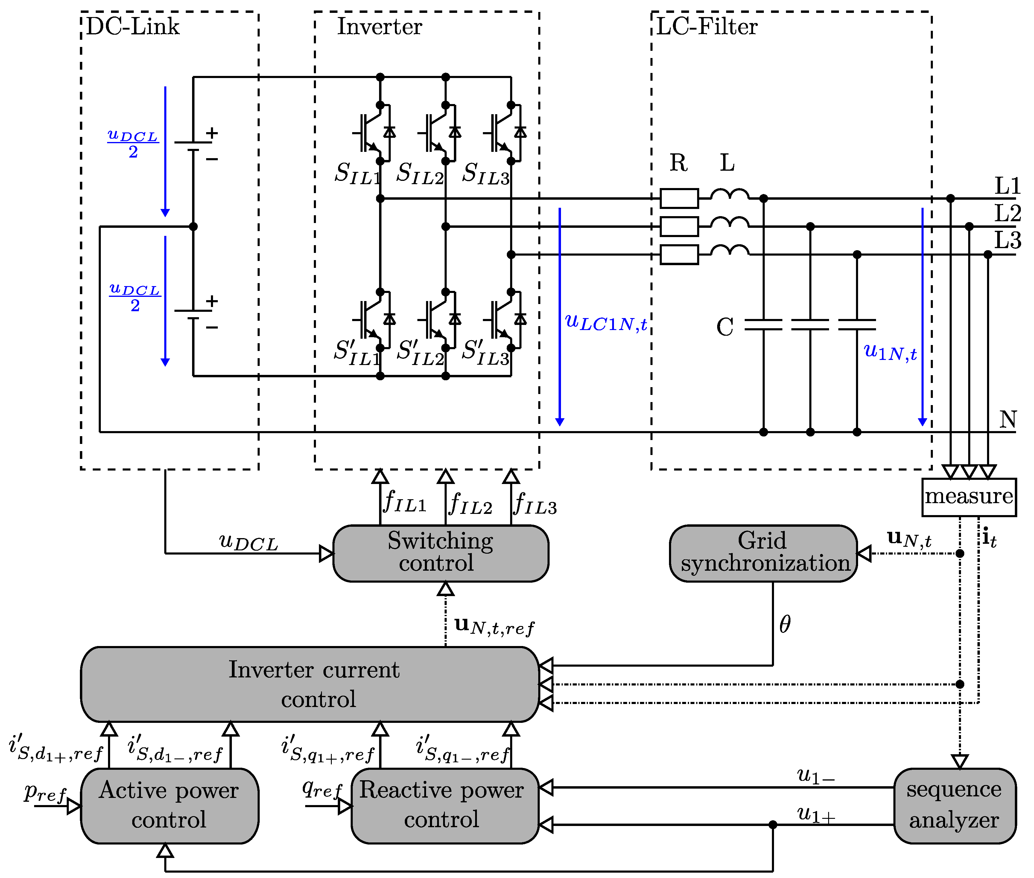
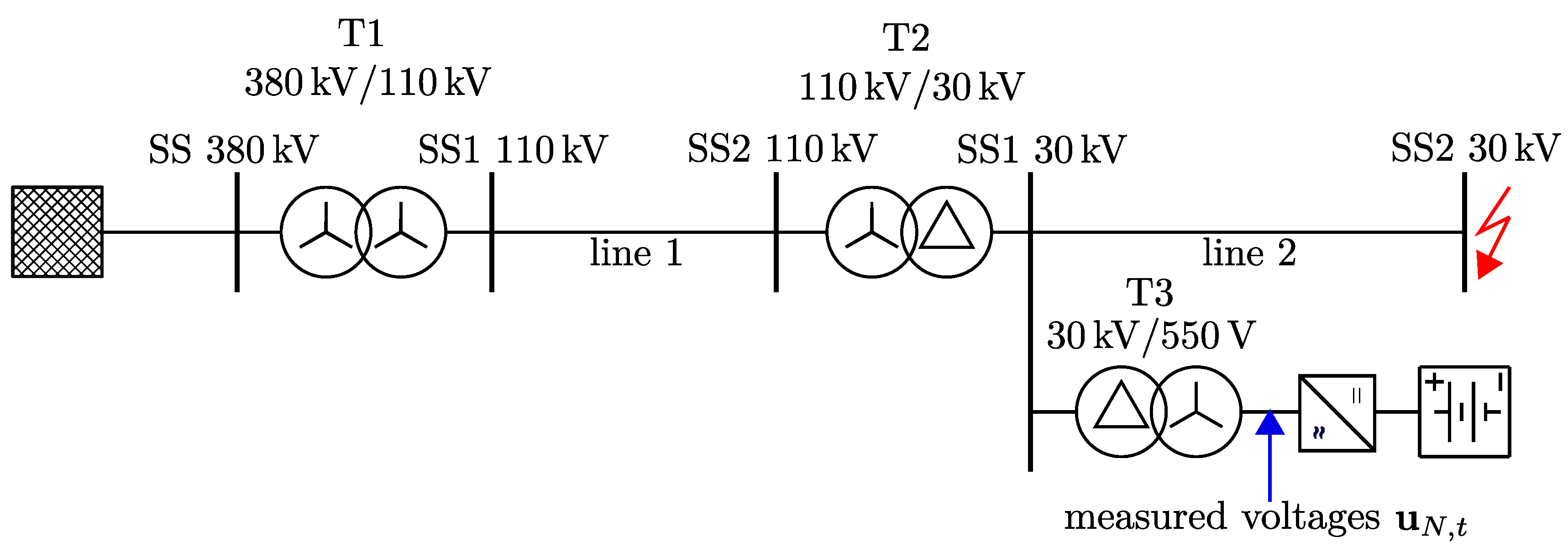
2.1. Description of the Model

Figure 3 shows the components and control structure of the converter used in the simulation model. The two-level voltage source converter model consists of a DC-link and an inverter which is followed by an LC-filter. For simplification, the DC-link is represented by a constant voltage source. The inverter model is a self-commutated three-phase bridge, which is controlled by a pulse-width-modulation (PWM) signal. The output filter consists of an LC-filter where the resistor represents the parasitic resistance of the inductance. The control structure follows a power-open-loop approach. Therefore, the current reference space vector ${\underline{i}}_{S,dq,ref}^{\prime }$ is directly calculated based on $\frac{p_{ref}}{u_{1+}}$ and $\frac{q_{ref}}{u_{1+}}$, assuming the converter during normal operation (no grid fault) to only inject active and reactive power in the positive-sequence system. The inverter current control is based on a double-synchronous reference frame (DSRF), where PI-controllers are used for the positive- as well as negative-sequence system to determine an instantaneous reference voltage vector ${\mathbf{u}}_{N,t,ref}$. The necessary transformations of the measured instantaneous voltage vector ${\mathbf{u}}_{N,t}$ and the measured instantaneous current vector ${\mathbf{i}}_t$ into the dq-plane, to determine the corresponding space vectors ${\underline{u}}_{S,dq}$ and ${\underline{i}}_{S,dq}$ are based on the angle $\theta$, which is provided by the grid synchronization. This grid synchronization is realized as an SRF-PLL. The switching control uses the instantaneous reference voltage vector ${\mathbf{u}}_{N,t,ref}$ to generate the PWM-signals $f_{IL1}$, $f_{IL2}$ and $f_{IL3}$ for the inverter, which control the switches $S_{IL1}$, $S_{IL2}$ and $S_{IL3}$. The complementary PWM-signals $f_{IL1}^{\prime }$, $f_{IL2}^{\prime }$ and $f_{IL3}^{\prime }$ are used to control the switches $S_{IL1}^{\prime }$, $S_{IL2}^{\prime }$ and $S_{IL3}^{\prime }$.

To describe the inverter current control in more detail, the requirements described in Section 1.1.2 are relevant. The injection of reactive currents according to Equations (1) and (2) require an estimation of the positive-sequence voltage $u_{1+}$ and the negative-sequence voltage $u_{1-}$. The “sequence analyzer” in Figure 3 performs this estimation by calculating these voltages. A description on how to calculate these voltages is given in Appendix A. As mentioned above, the simulation model is based on a power open-loop approach. The corresponding reference values for active and reactive power are calculated inside the “active power control” and “reactive power control”, respectively. During normal operation (no grid fault) the reactive power control calculates the corresponding current reference value $i_{S,q_{1+},ref}^{\prime }$ according to the reference power $q_{ref}$:

$$\begin{array}{cc}\hfill i_{S,q_{1+},ref}^{\prime }& =\frac{q_{ref}}{u_{1+}}\hfill \end{array}$$

(18)

It is assumed that during normal operation reactive power is only injected in the positive-sequence system, therefore, the reference value $i_{S,q_{1-},ref}^{\prime }=0$ is zero. During a grid fault, the reference values are calculated based on Equations (1) and (2):

$$\begin{array}{cc}\hfill i_{S,q_{1+},ref}^{\prime }\left(t\right)& =i_{S,q_{1+},ref}^{\prime }\left(T_{gf}\right)+k_{1+}·\Delta u_{1+}\left(t\right)\hfill \end{array}$$

(19)

$$\begin{array}{cc}\hfill i_{S,q_{1-},ref}^{\prime }\left(t\right)& =k_{1-}·\Delta u_{1-}\left(t\right)\hfill \end{array}$$

(20)

The “active power control” calculates the current reference value $i_{S,d_{1+},ref}^{\prime }$ as follows

$$\begin{array}{cc}\hfill i_{S,d_{1+},ref}^{\prime }& =\frac{p_{ref}}{u_{1+}}\hfill \end{array}$$

(21)

The power control is followed by the inverter current control, which is shown in Figure 4.

It consists of two parts: the “current limitation” and the actual current controller. The current limitation implements the explanations described in Section 1.2. The pseudo-code in Algorithm 1 shows the actual implementation of the current limitation.

Algorithm 1: Implementation of a current limitation according to Section 1.2

The current limitation is followed by a “negative-sequence transformation”. This block is necessary to take into account the angle ${\phi }_{\pm }$ shown in Figure 2. The PLL provides the angle $\theta$, which represents the angle of the positive-sequence voltage space vectors ${\underline{u}}_{S,d{q}_{1+}}$. As the components $i_{S,d_{1-}}$ and $i_{S,q_{1-}}$ are given with reference to the $\alpha \beta$-plane in the negative-sequence system, they have to be transformed in the $\alpha \beta$-plane in the positive-sequence system accordingly, as already shown in Equation (9):

$$\begin{array}{c}\hfill {\underline{i}}_{S,d{q}_{1-}}^{\prime }{e}^{-j\omega t}{e}^{j{\phi }_{\pm }}\end{array}$$

(22)

where

$$\begin{array}{cc}\hfill {\phi }_{\pm }& =arg(u_{S,d_{1-}}+j{u}_{S,q_{1-}})\hfill \end{array}$$

(23)

This transformation is performed by the “negative-sequence transformation”.

The actual current controller is based on four PI-controllers for each component of the (limited) reference currents $i_{S,d_{1+},ref}$, $i_{S,q_{1+},ref}$, $i_{S,d_{1-},ref}$ and $i_{S,q_{1-},ref}$. To determine the corresponding current components that are currently injected at the output of the converter, these components have to be extracted from the measured phase currents ${\mathbf{i}}_t$. To do this, the park-transformation is followed by Notch-filters which are tuned to $2\omega$. The occurrence of negative-sequence components leads to a second harmonic in the positive-sequence dq-components. This is also the case for the negative-sequence components when a positive-sequence occurs. By using park-transformations for the positive-sequence system ($+\theta$) and for the negative-sequence system ($-\theta$), where each component of the dq-output is followed by a Notch-filter tuned to $2\omega$, these second harmonics can be filtered. The differences of the measured components {$i_{S,d_{1+}}$, $i_{S,q_{1+}}$, $i_{S,d_{1-}}$, $i_{S,q_{1-}}$} and {$i_{S,d_{1+},ref}$, $i_{S,q_{1+},ref}$, $i_{S,d_{1-},ref}$, $i_{S,q_{1-},ref}$} are used as input for the corresponding PI-controllers. Between the voltage at the output of the inverter ${\mathbf{u}}_{LC,t}$ and the voltage output of the whole converter ${\mathbf{u}}_{N,t}$, a voltage drop over the LC-filter occurs. This voltage drop has to be considered in the inverter current control. The voltage drop over the LC-filter is taken into account by using the normalized inductance l

$$\begin{array}{cc}\hfill l& =\frac{{\omega }_n·L}{\frac{U_n^2}{S_n}}\hfill \end{array}$$

(24)

with the equation

$$\begin{array}{cc}\hfill {\underline{u}}_{LC,S,dq}& ={\underline{u}}_{S,dq}+j\frac{\omega }{{\omega }_n}l·{\underline{i}}_{S,dq}=(u_{S,d}+i_{S,d}R-\frac{\omega }{{\omega }_n}l·i_{S,q})+j(u_{S,q}+i_{S,q}R+\frac{\omega }{{\omega }_n}l·i_{S,d})\hfill \end{array}$$

(25)

that is valid for both sequence systems. To extract the components of the voltage space vector ${\underline{u}}_{S,dq}$ out of the measured voltages ${\mathbf{u}}_{N,t}$, the same approach as for the currents is used, which consists of a park-transformation followed by Notch-filters, each for the positive- and negative-sequence systems.

2.2. LC-Filter Design Considerations and Tuning of the Inverter Current Control

Due to the fast-switching inverter, an output filter is necessary to smooth the AC output currents. A series inductance accomplishes this task. Its value is determined as the maximum AC current ripple $\Delta I_{rip}$ that is allowed at the converter output. According to Teodorescu et al. [8], a rough approximation of the value of this inductance can be calculated by

$$\begin{array}{cc}\hfill L& =\frac{U_{DCL}}{2·\Delta I_{rip}·f_{sw}}\hfill \end{array}$$

(26)

for two-level PWM converters, where $f_{sw}$ is the switching frequency of the switching control. The use of the capacitors is justified by the necessity to filter the switching frequency harmonics. In case the capacitor voltage is sensed, as shown in Figure 3, a part of the reactive power of the inductances will be compensated by the capacitors with a consequent decrement of the power factor seen at the PCC. According to Beres et al. [19], the value of the capacitors can be determined based on

$$\begin{array}{cc}\hfill C& =0.05·\frac{1}{{\omega }_n\frac{U_n^2}{S_n}}\hfill \end{array}$$

(27)

where $S_n$ is the nominal apparent power of the converter.

The tuning of the PI-controllers shown in Figure 4 can be done according to [20]. The decoupling $\frac{\omega }{{\omega }_n}l$-terms in Figure 4 guarantee the direct/active and quadrature/reactive components in the positive- as well as negative-sequence system to be decoupled. Therefore, a change of reference values of a certain component only influences the corresponding output component. For example, a change of $i_{S,d_{1+},ref}$ only has an influence on $i_{S,d_{1+}}$ and not on $i_{S,q_{1+}}$ or any other component. Each of the four components can, therefore, be considered as a single-input single-output system. In the Laplace domain, the PI-controllers are represented by

$$\begin{array}{cc}\hfill R_I\left(s\right)& =K_P+\frac{K_I}{s}\hfill \end{array}$$

(28)

and the process function can be approximated by neglecting the transfer function of the switching control and the inverter with

$$\begin{array}{cc}\hfill G_I\left(s\right)& =\frac{\frac{1}{R}}{1+s\frac{L}{R}}\hfill \end{array}$$

(29)

resulting in a loop gain of

$$\begin{array}{cc}\hfill L_I\left(s\right)& =R_I\left(s\right)G_I\left(s\right)=\frac{K_P}{sL}·\frac{s+\frac{K_I}{K_P}}{s+\frac{R}{L}}\hfill \end{array}$$

(30)

By choosing $K_P=\frac{L}{{\tau }_i}$ and $K_I=\frac{R}{{\tau }_i}$, the closed-loop transfer function $\frac{L_I\left(s\right)}{1+L_I\left(s\right)}$ has a PT1-behavior with a freely selectable time constant ${\tau }_i$. A corresponding choice of L and C and the gains $K_P$ and $K_I$ for each of the four current control loops shown in Figure 4 is summarized in

Table 1. Parameters of the converter model and its control used in the simulation.

Parameter	Value
$U_n$	550 $\mathrm{V}$
$S_n$	650 kVA
$U_{DCL}$	900 $\mathrm{V}$
$f_{sw}$	8 $\mathrm{k}$$\mathrm{Hz}$
L	280 $\mathsf{\mu }$$\mathrm{H}$
R	1 $\mathrm{m}$$\mathsf{\Omega }$
C	342 $\mathsf{\mu }$$\mathrm{F}$
${\widehat{i}}_{max}$	$1.1$ pu
${\tau }_i$	20 $\mathsf{\mu }$$\mathrm{s}$
$K_P$	14 pu
$K_I$	50 pu

.

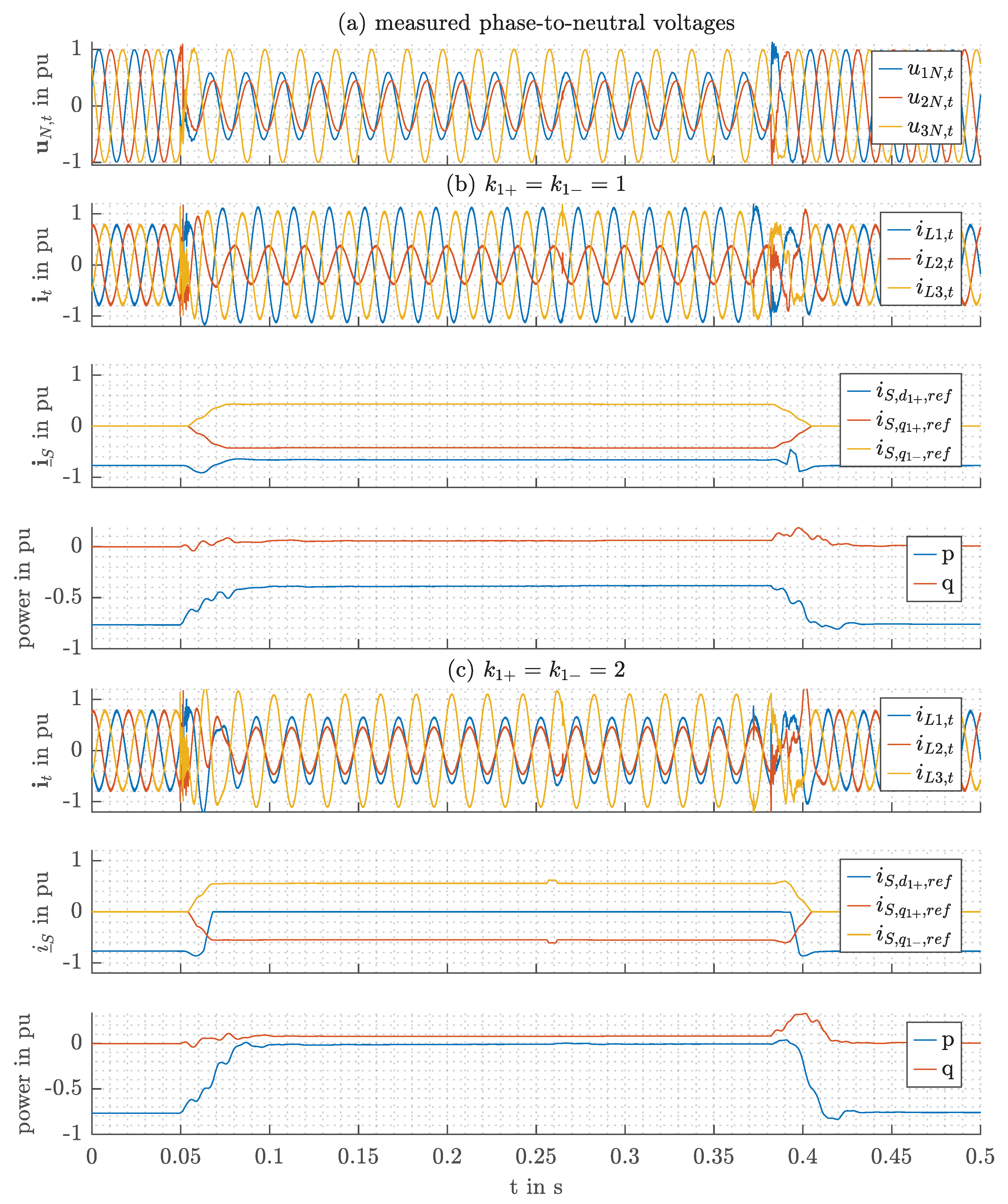
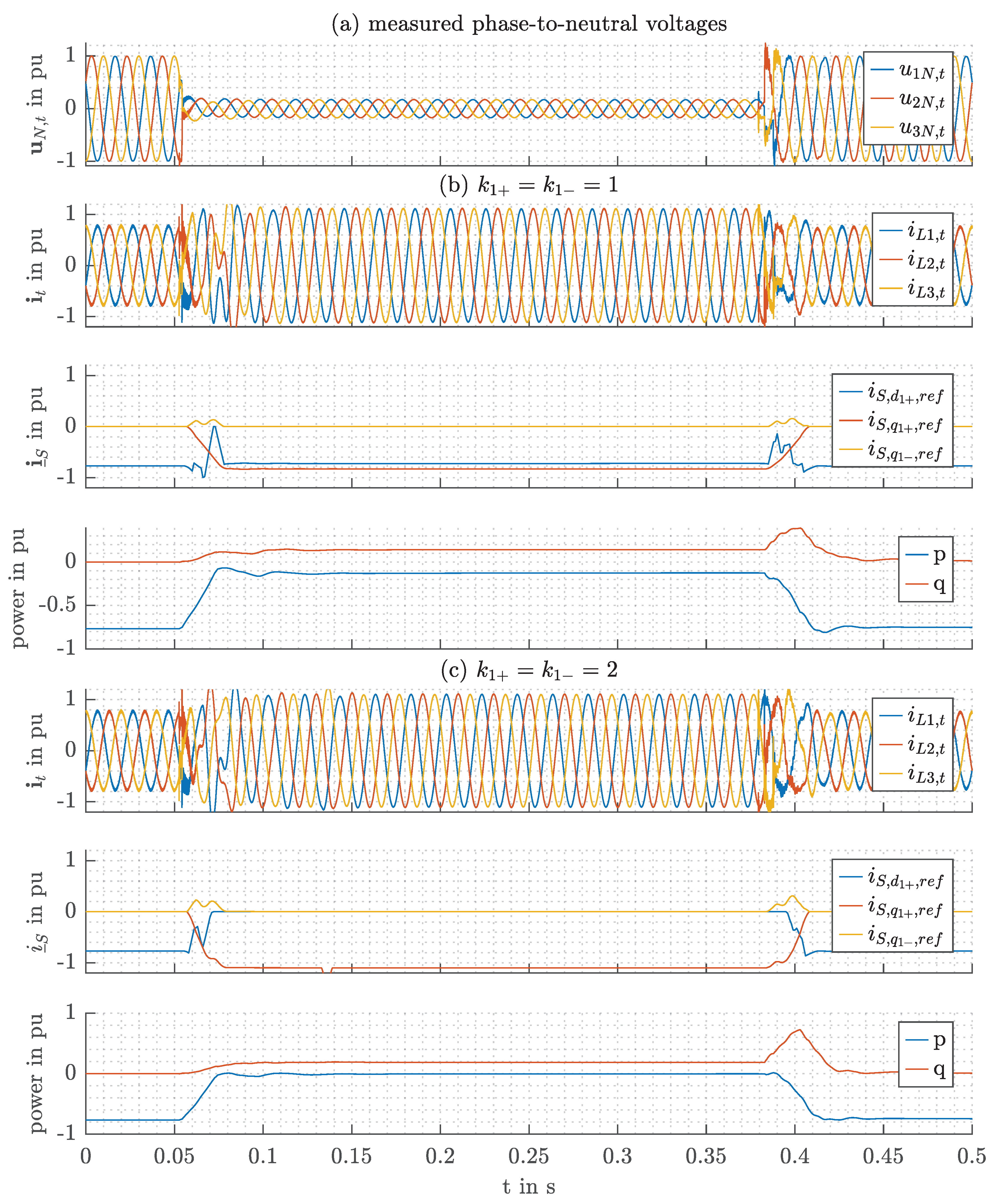
2.3. Application of the Model

In [16,21], the LVRT-behavior and the dynamic voltage support of a battery-converter during real faults in a feeder were investigated. Forced balanced (symmetrical) and unbalanced (asymmetrical) faults in the upstream 110 $\mathrm{k}$$\mathrm{V}$ and 30 $\mathrm{k}$$\mathrm{V}$ grids were carried out and measured by suitable measurement equipment. The corresponding single-line diagram of the short-circuits carried out is shown in Figure 5. These measurements are used as input of the model presented above by using the measured voltage as the input of a controlled voltage source connected to the converter model shown in Figure 3.

The parameters of the converter model shown in Figure 3 and the gains of the current controller shown in Figure 4 are summarized in Table 1. Two test cases are selected out of the available measurements, which are based on a two-phase short-circuit and a three-phase short-circuit in the upstream 30 $\mathrm{k}$$\mathrm{V}$ grid. There is an impedance between the measuring point, which was the PCC of the battery converter, and the fault point, which leads to a residual voltage at the measurement point during a fault. This residual voltage determines the behavior of the battery converter according to Equations (1) and (2). Based on the simulation model presented above, this behavior is simulated. For both test cases, the two factors $k_{1+}$ and $k_{1-}$ are chosen out of {1,2} for simulation. A maximum current capability of ${\widehat{i}}_{max}=1.1 \mathrm{pu}$ is assumed.

Figure 6 shows the corresponding simulation results for the two-phase short-circuit.

The measured voltage according to Wurm [16] is shown in Figure 6a. Figure 6b,c shows the simulation results for $k_{1+}=k_{1-}=1$ and $k_{1+}=k_{1-}=2$. The results consist of the phase current output ${\mathbf{i}}_t$, the reference current space vector ${\underline{i}}_S$ consisting of the current components $i_{S,d_{1+},ref}$, $i_{S,q_{1+},ref}$, $i_{S,q_{1-},ref}$ and the active power output p and the reactive power output q of the converter. At the beginning of the simulation, it is assumed that the converter feeds in active power at an operating point of $p=-0.77 \mathrm{pu}$, $q=0 \mathrm{pu}$. At $T_{gf}=50 \mathrm{m}\mathrm{s}$, the two-phase short-circuit in the upstream 30 $\mathrm{k}$$\mathrm{V}$ grid leads to a drop in the positive-sequence voltage $u_{1+}$ and a rise in the negative-sequence voltage $u_{1-}$. According to Equations (1) and (2), the converter starts to inject reactive current. The corresponding reference current components are shown in Figure 6b,c. Since the load-reference system is used, the drop in positive-sequence voltage leads to a negative reference current component $i_{S,q_{1+},ref}$, while the rise in negative-sequence voltage leads to a positive reference current component $i_{S,q_{1-},ref}$. In the case of Figure 6c, the current components are higher than in Figure 6b, due to the higher values of $k_{1+}$ and $k_{1-}$. According to Algorithm 1, the active current component $i_{S,d_{1+},ref}$ has to be limited so that the maximum phase current ${\widehat{i}}_{max}$ is respected. In Figure 6c, the reactive current components do have such high values that the active current component has to be limited to zero and also the reactive current components have to be limited. In Figure 6b, only the active current component is limited. In both cases, the current output ${\mathbf{i}}_t$ in Figure 6b,c shows that the maximum current capability of ${\widehat{i}}_{max}$ is respected. Due to this limitation, the active power p in Figure 6b is reduced. Because reactive currents are injected into both the positive- and negative-sequence systems, and they have opposite sign, the reactive power q in Figure 6b is only slightly higher than zero. In Figure 6c, the active power p is reduced to zero and the reactive power q is slightly higher than in Figure 6b.

Figure 7 shows the corresponding simulation results for the three-phase short-circuit.

The measured voltage according to Wurm [16] is shown in Figure 7a. Figure 7b,c shows the simulation results for $k_{1+}=k_{1-}=1$ and $k_{1+}=k_{1-}=2$. The results consist of the phase current output ${\mathbf{i}}_t$, the reference current space vector ${\underline{i}}_S$ consisting of the current components $i_{S,d_{1+},ref}$, $i_{S,q_{1+},ref}$, $i_{S,q_{1-},ref}$ and the active power output p and the reactive power output q of the converter. At the beginning of the simulation it is assumed that the converter feeds in active power at an operating point of $p=-0.77 \mathrm{pu}$, $q=0 \mathrm{pu}$. At $T_{gf}=50 \mathrm{m}\mathrm{s}$, the two-phase short-circuit in the upstream 30 $\mathrm{k}$$\mathrm{V}$ grid leads to a drop in the positive-sequence voltage $u_{1+}$. The negative-sequence voltage $u_{1-}$ stays at zero. According to Equation (1), the converter starts to inject reactive current. The corresponding reference current components are shown in Figure 7b,c. Since the load-reference system is used, the drop in positive-sequence voltage leads to a negative reference current component $i_{S,q_{1+},ref}$. The current component $i_{S,q_{1-},ref}=0$ is zero, because there is no change of the negative-sequence voltage ($\Delta u_{1-}=0$). According to Algorithm 1, the active current component $i_{S,d_{1+},ref}$ has to be limited so that the maximum phase current ${\widehat{i}}_{max}$ is respected. In Figure 7c, the reactive current component $i_{S,q_{1+},ref}$ does have such high values that the active current component has to be limited to zero and the reactive current component must also be limited. In (b), only the active current component has to be limited. In both cases, the current output ${\mathbf{i}}_t$ in Figure 6b,c shows that the maximum current capability of ${\widehat{i}}_{max}$ is respected. Due to this current limitation, the active power p in Figure 7b is reduced and limited to zero in (c). Due to the low voltage ${\mathbf{u}}_{N,t}$ during the fault, the reactive power only reaches low values of about $0.15$ pu in Figure 7b and about $0.2$ pu in Figure 7c.

3. Conclusions

This paper investigates the dynamic voltage support of converters during grid faults, which is required by national grid codes in Austria and many other countries. A converter model was created in the software MATLAB/SIMULINK to simulate the behavior of converters during grid faults. The converter control in this simulation model applies a current limitation algorithm, which is also presented in this paper. This current limitation algorithm takes into account the requirements of grid codes, which include the injection of reactive current in the positive- as well as negative-sequence system, directly proportional to the change of the corresponding voltage between fault and pre-fault. Together with the active current components, this results in four different reference current components, which are limited by the current limitation algorithm according to the requirements in the grid codes in order to respect the maximum current capability of the converter.

The simulation model is used to investigate the behavior of a converter based on voltage measurements, which were taken during forced short-circuits in a real 30 $\mathrm{k}$$\mathrm{V}$ grid. Two test cases were investigated, which are based on the voltage measurement during a two-phase short-circuit and a three-phase short-circuit. Within these test cases, the proportional factor which determines the value of reactive current injection is varied. The results in all simulations show that the presented algorithm for current limitation is capable of guaranteeing a current output below the maximum current capability.

Compared to existing approaches for current limitation during dynamic voltage support, the current limitation algorithm proposed in this paper has the advantage that it can meet the grid code requirements also in the case of current saturation during the sole injection of reactive power. National grid codes require an even reduction of the reactive current components in the positive- and negative-sequence systems in such a case. This requirements are taken into account by the current limitation algorithm proposed in this paper. However, the simplified converter model used in the simulation does not specifically model the DC-link of a converter. Therefore, the simulation results are limited to the AC-side of the converter.

Future research goals include the extension of the used converter model by a specific DC-link representation, the implementation of the proposed current limitation algorithm on a real converter system and investigation of experiments on this system.

References

1. Erlich, I.; Neumann, T.; Shewarega, F.; Schegner, P.; Meyer, J. Wind turbine negative sequence current control and its effect on power system protection. In Proceedings of the 2013 IEEE Power & Energy Society General Meeting, Vancouver, BC, Canada, 21–25 July 2013; pp. 1–5. [Google Scholar]
2. VDE. VDE-AR-N 4110: Technische Regeln für den Anschluss von Kundenanlagen an das Mittelspannungsnetz und deren Betrieb (TAR Mittelspannung). 2017. Available online: https://www.vde.com/de/fnn/arbeitsgebiete/tar/tar-mittelspannung-vde-ar-n-4110 (accessed on 9 May 2020).
3. E-Control. Technische und organisatorische Regeln für Betreiber und Benutzer von Netzen: TOR Erzeuger: Anschluss und Parallelbetrieb von Stromerzeugungsanlagen des Typs B. 2019. Available online: https://www.e-control.at/documents/1785851/1811582/TOR+Erzeuger+Typ+B+V1.0.pdf/a9a7e5ae-5842-caa9-d2c0-93be4b6e0802?t=1562757801048 (accessed on 9 May 2020).
4. Castilla, M.; Miret, J.; Sosa, J.L.; Matas, J.; de Vicu na, L.G. Grid-fault control scheme for three-phase photovoltaic inverters with adjustable power quality characteristics. IEEE Trans. Power Electron. 2010, 25, 2930–2940. [Google Scholar] [CrossRef]
5. Chaudhary, S.K.; Teodorescu, R.; Rodriguez, P.; Kjaer, P.C.; Gole, A.M. Negative sequence current control in wind power plants with VSC-HVDC connection. IEEE Trans. Sustain. Energy 2012, 3, 535–544. [Google Scholar] [CrossRef]
6. Mortazavian, S.; Shabestary, M.M.; Mohamed, Y.A.R.I. Analysis and dynamic performance improvement of grid-connected voltage–source converters under unbalanced network conditions. IEEE Trans. Power Electron. 2016, 32, 8134–8149. [Google Scholar] [CrossRef]
7. Camacho, A.; Castilla, M.; Miret, J.; Borrell, A.; de Vicu na, L.G. Active and reactive power strategies with peak current limitation for distributed generation inverters during unbalanced grid faults. IEEE Trans. Ind. Electron. 2014, 62, 1515–1525. [Google Scholar] [CrossRef] [Green Version]
8. Teodorescu, R.; Liserre, M.; Rodriguez, P. Grid Converters for Photovoltaic and Wind Power Systems; John Wiley & Sons: Hoboken, NJ, USA, 2011; Volume 29. [Google Scholar]
9. Jia, J.; Yang, G.; Nielsen, A.H. Investigation of grid-connected voltage source converter performance under unbalanced faults. In Proceedings of the 2016 IEEE PES Asia-Pacific Power and Energy Engineering Conference (APPEEC), Xi’an, China, 25–28 October 2016; pp. 609–613. [Google Scholar]
10. Du, X.; Wu, Y.; Gu, S.; Tai, H.M.; Sun, P.; Ji, Y. Power oscillation analysis and control of three-phase grid-connected voltage source converters under unbalanced grid faults. IET Power Electron. 2016, 9, 2162–2173. [Google Scholar] [CrossRef]
11. Rodriguez, P.; Timbus, A.V.; Teodorescu, R.; Liserre, M.; Blaabjerg, F. Flexible active power control of distributed power generation systems during grid faults. IEEE Trans. Ind. Electron. 2007, 54, 2583–2592. [Google Scholar] [CrossRef]
12. López, M.A.G.; de Vicu na, J.L.G.; Miret, J.; Castilla, M.; Guzmán, R. Control strategy for grid-connected three-phase inverters during voltage sags to meet grid codes and to maximize power delivery capability. IEEE Trans. Power Electron. 2018, 33, 9360–9374. [Google Scholar] [CrossRef] [Green Version]
13. Shin, D.; Lee, K.J.; Lee, J.P.; Yoo, D.W.; Kim, H.J. Implementation of fault ride-through techniques of grid-connected inverter for distributed energy resources with adaptive low-pass notch PLL. IEEE Trans. Power Electron. 2014, 30, 2859–2871. [Google Scholar] [CrossRef]
14. Göksu, Ö.; Teodorescu, R.; Bak, C.L.; Iov, F.; Kjær, P.C. Impact of wind power plant reactive current injection during asymmetrical grid faults. IET Renew. Power Gener. 2013, 7, 484–492. [Google Scholar] [CrossRef]
15. Taul, M.G.; Wang, X.; Davari, P.; Blaabjerg, F. Current reference generation based on next generation grid code requirements of grid-tied converters during asymmetrical faults. IEEE J. Emerg. Sel. Top. Power Electron. 2019. [Google Scholar] [CrossRef] [Green Version]
16. Wurm, M. 110-und 30-kV-Netzkurzschlussversuche mit einem 2, 2-MWh-Batteriespeicher. E I Elektrotechnik Und Inf. 2019, 136, 21–30. [Google Scholar] [CrossRef]
17. European Union. Commission Regulation (EU) 2016/631; Establishing a Network Code on Requirements for Grid Connection of Generators (RfG). 2016. Available online: http://data.europa.eu/eli/reg/2016/631/oj (accessed on 9 May 2020).
18. IEC 60909-0:2016. Short-Circuit Currents in Three-Phase a.c. Systems—Part 0: Calculation of Currents. 2016. Available online: https://webstore.iec.ch/publication/24100 (accessed on 9 May 2020).
19. Beres, R.N.; Wang, X.; Liserre, M.; Blaabjerg, F.; Bak, C.L. A review of passive power filters for three-phase grid-connected voltage-source converters. IEEE J. Emerg. Sel. Top. Power Electron. 2015, 4, 54–69. [Google Scholar] [CrossRef] [Green Version]
20. Yazdani, A.; Iravani, R. Voltage-Sourced Converters in Power Systems: Modeling, Control, and Applications; John Wiley & Sons: Hoboken, NJ, USA, 2010. [Google Scholar]
21. Marchgraber, J.; Gawlik, W.; Wurm, M. Modellierung der dynamischen Netzstützung von über Umrichter angebundenen Erzeugungsanlagen und Speichern. E I Elektrotechnik Und Inf. 2019, 136, 31–38. [Google Scholar] [CrossRef] [Green Version]
22. FGW. Technische Richtlinien für Erzeugungseinheiten und -anlagen; Teil 3 (TR3); Bestimmung der elektrischen Eigenschaften von Erzeugungseinheiten und -anlagen am Mittel-, Hoch- und Höchstspannungsnetz. 2017. Available online: https://wind-fgw.de/wp-content/uploads/2018/10/FGW/Teil3/Rev25/preview/180901-1.pdf (accessed on 9 May 2020).
Figure 1. LVRT-curve for Type B non-synchronous power-generating modules (power park modules) in Austria [3]. The minimum phase-to-phase voltage at the PCCR is relevant to the decision of whether a module is allowed to disconnect or not. The LVRT-curve is valid both for symmetrical as well as asymmetrical grid faults. The starting point of the LVRT-curve is defined as T g f , which is described in Equation (6).
Energies 13 02484 g001
Figure 2. Vector diagram to derive the calculation for the current limitation (valid only for ω t = 0 ).
Energies 13 02484 g002
Figure 3. Converter and its control routines used in the simulation model.
Energies 13 02484 g003
Figure 4. “Inverter current control”-block of Figure 3, using a double synchronous reference frame (DSRF) with notch filters (NF) based on [8]. The current limitation implements the explanations in Section 1.2 (R of Equation (25) is neglected).
Energies 13 02484 g004
Figure 5. Single-line diagram of the short-circuit location from which measurements are used for simulation.
Energies 13 02484 g005
Figure 6. Simulation results of a two-phase short-circuit (the load reference system is used).
Energies 13 02484 g006
Figure 7. Simulation results of a three-phase short-circuit (the load reference system is used).
Energies 13 02484 g007