Abstract
With the progressive addition of microgrids at the distribution level, complex networks of interconnected microgrids and the utility grid are likely to emerge. In such a scenario, advanced microgrid controllers are required to achieve operational stability objectives while maintaining a cost-effective operation. This paper investigates the control strategies, trading mechanisms, and interconnection configurations of a multi-microgrid and utility grid system for frequency stability analysis and operational cost optimization. The analysis is performed on a model of two interconnected microgrids and the utility grid, all possible interconnection configurations are tested. A robust controller is designed and the control parameters are later optimized to ensure that the frequency stability of the system is maintained under normal operating conditions and under various disturbances. A new control element based on switching between interconnection configurations is introduced to handle the power that flows between microgrids, aiming to minimize inter-microgrid energy trading cost while maintaining the system frequency fluctuations within tolerance levels. The effectiveness of the designed controller is demonstrated in this work. This work is expected to provide new insights in the field of multi-microgrid system design.
1. Introduction
Several factors, including environmental concerns, power grid modernization, and access to power in underdeveloped or remote areas, have stimulated extensive research in the area of renewable energy and distributed generations. Microgrid (MG) and associated technologies have been developed as a promising solution. MG typically consists of electric loads, various types of distributed generators (DGs) including wind turbine generators (WTGs), solar photovoltaic (PV) units, microturbines (MTs), and in some cases electrolyzer (ES), fuel cells (FC), and various types of energy storage systems [1]. MGs can operate in several modes: (1) interconnected to other MGs (but disconnected from the utility grid (UG)), (2) connected only to the utility grid (UG), (3) connected simultaneously to other MGs and the UG, and (4) disconnected from other MGs and the UG (island mode). In an alternate current (AC) MG, its connection to neighboring MGs and the UG are mainly for operational cost reduction and improved reliability and stability. Through energy trading, an MG can take advantage of the diversity of supplies and demands in neighboring MGs and UG to achieve a mutual benefit while meeting system stability requirements [2]. Given the stochastic nature of electrical loads, the variable power output of solar PV and WTG generators, the diverse MG operational modes, and the highly complex interactions between interconnected MGs and the UG, it is advised to use an optimal robust microgrid controller (MGC) to achieve power quality goals.
For an MG illustrated in Figure 1, proportional-integral (PI) controllers are proposed to adjust MT (generation) and ES (load) to minimize the power imbalances and the resulting frequency fluctuations in both island and grid-connected modes [3]. In [4], the proposed MG, the PV, WTG, and loads are generally stochastic and passively monitored by the MGC. In [5], a similar MG was studied, and particle swarm optimization (PSO) algorithm was implemented to select the appropriate PI controller parameters. Linear [6] and nonlinear [7] droop controls were also developed to optimize MG operation. Therefore, in the case of a single MG, optimal robust MGC has been well-established. To simulate the dynamic behavior of MG components, a simple but widely adopted [3,4,5,8] microgrid modeling technique was applied. This approach outputs a fair approximation of the dynamic response of the system, needed to generate valid conclusions for the work.
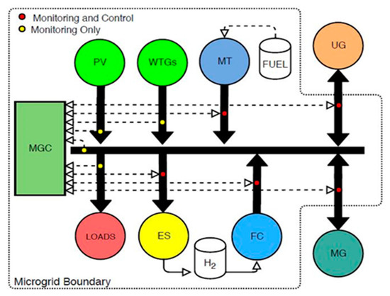
Figure 1.
Configuration of an individual microgrid (MG) and microgrid controller (MGC). Reprint with permission [11]; 2019, IEEE.
Hao et al. [9] and Jadhav et al. [10], investigated a system of three interconnected MGs, with one of the MGs connected to the UG through a passive link. A variety of components including a battery energy storage system (BESS), flywheel energy storage, diesel generators, heat pumps, and electric vehicles (EVs) were added in the model. Operation costs were included as part of the optimization objectives [9]. Voltage stability was also considered in MGC design [10]. The concepts of energy internet and power router were discussed. However, the system under study was essentially one large MG with a fixed configuration and UG connection. It is of both theoretical and practical interests to explore the possible consequences of variable or flexible configurations. As shown in Figure 2, the power lines that connect the two MGs between them and with the UG are switchable, meaning that the lines can be connected or disconnected by the controller to improve frequency stability and/or to reduce the operational cost.
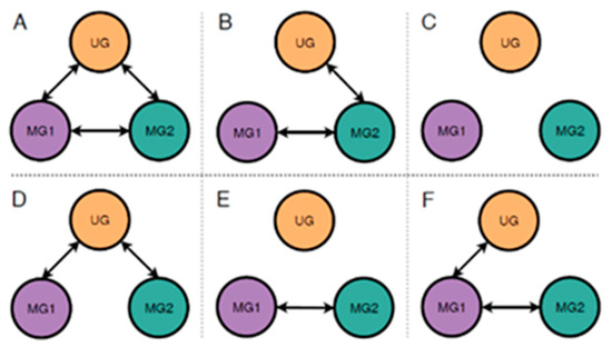
Figure 2.
Possible interconnection configurations (shown by arrows) for 2 MGs and the utility grid (UG). Reprint with permission [11]; 2019, IEEE.
In recent years, the economic operation of multi-MG systems has attracted plenty of research attention. Hussain et al. [12] proposed a method for energy trading between microgrids located in a distribution network. Key elements of their approach included a simple pricing mechanism and a mediator protecting buyer and seller interests. Park et al. [13] introduced a new energy management system for networked MGs. The objective for island operation and grid-connected modes was to minimize operating costs. The time horizon for the analysis was day-ahead. Wang et al. [14], proposes, for networked MGs, a “distributor” which collects all energy surplus from any MG and then distributes it to others based on each MG’s historical contribution and the maximization of each consumer’s utility. Wu et al. [15] proposes a bilevel approach to energy management in MG networks. With a distribution network operator in the first level and multiple MGs in the second level, the objective is to minimize overall operating costs. Kou et al. [16], presented a decentralized optimal control algorithm by considering the distribution network as a collection of coupled MGs. Each MG in the distribution system must share information with the rest. Individual MG controllers use local information as well as the received information to select the right trading action to achieve local and global objectives. In Gregoratti and Matamoros [17] work, a group of neighboring MGs in the same distribution network trade power based on the information collected and shared by a DNO. The distributed economic model predictive control is developed to coordinate the multi-MG system under uncertainty. Zhao et al. [18], proposed a distributed dual decomposition algorithm controller for a group of MGs not connected to the utility grid, each MG has a generation cost, the cost of network utilization is also considered. The objective is to find the optimal amount of traded energy that will minimize overall operational costs. Wang and Huang [19], used an energy management system to solve the problem of unbalanced supply and demand. The optimization was performed on two levels, individual MG level, and multi-MG level. The coordinated operation is preferable since it was shown that while individual MGs can achieve local objectives, the whole system could have an expensive operation cost. Bullich-Massagué et al. [20], used a decentralized algorithm method with minimum information exchange to coordinate inter-MG energy trading. The case study demonstrated that, through energy trading, an individual MG reduced its operation cost by up to 29.4% and all MGs in the system reduced the overall cost by 13.2%. Gazijahani et al. [21] presents a summary of interconnection architectures for multi-MG systems along with comparisons of cost, stability, protection, scalability, reliability, communications, and business models. Arefifar et al. [22] presents a risk-based multi-objective approach for energy exchange optimization among networked MGs. The authors also suggest that coordinated MGs can achieve reduced operational costs. In our previous work [11], a centralized day-ahead energy management system for interconnected MGs that aims to minimize operating cost is used to define the optimal value of the decision variables (dispatchable generation).
Most of the relevant literature indicates that energy management or coordination at the inter-MG level can help achieve reduced operational costs. However, the research attention has been given mainly to the economic aspects such as operational costs rather than system stability (it was assumed that MGs can always self-stabilize). The main contributions of this work are as follows:
- Development of a multi-MG simulation framework with the capability of optimizing MG controller parameters for frequency stability. Implemented in MATLAB/SIMULINK, the controller parameter selection is much more important and consequential in the case of islanded MGs. For interconnected MGs, it is found that joint optimization of the parameters of the controllers of all MGs can help reduce system frequency deviation.
- Investigation of three different power trading mechanisms between MGs, namely, natural, conservative, and active trading mechanisms. For each mechanism, we tested the frequency deviations under disturbances and demonstrate their respective advantages. The results regarding frequency stability with these mechanisms are novel and of relevance and may serve as “limiting cases” for other more advanced trading mechanisms.
- Comparison of MG operation costs under different interconnection configurations and trading mechanisms. On the one hand, it is suggested that given the UG price signal and the multi-MG system operational characteristics, cost performance can be improved when switching to other interconnection configurations. On the other hand, it is also shown that at least in some cases there is a trade-off between cost reduction and frequency stability.
The specific innovative part of this work compared to similar studies can be summarized as three power trading mechanisms in combination with different interconnection configurations that are used to improve frequency stability and operational cost of interconnected MGs. The other sections of this paper are organized as follows. Section 2 describes the model formulation, model parameters, and the three trading mechanisms. Section 3 presents the results on the frequency stability of single MG and two connected MG, as well as the operational costs in different scenarios. The conclusions are stated in Section 4.
2. Methodology
In this section, a model of two interconnected MGs and the UG was presented. The main control of the system was achieved through PI controllers within each MG. For each mode of operation, a control objective was presented. In the grid-tie mode, the control objective was to minimize power from UG while minimizing power mismatch at the MG bus. In the island mode, the MG controller objective was to minimize power mismatch at the MG bus.
2.1. Model Formulation
The control system schematic of a single MG is presented in Figure 3. To minimize power mismatch on the MG, the generation must match the demand as described in the next equation:
where is the power deviation at the MG bus, is the total power generation and is the total power demand. and are further described in the following Equations (2) and (3):
where is the power from the WTGs, is the power output of the solar PV system, is the power output of the FC, is the power output of the MT, is the power from and to the UG, is power from and to the neighboring MG, is the power demand of the MG load, and is the power demand of ES. generations and demand are within respective bounds as detailed in Table 1. and are not constrained. Initial values for the model are given in Table 1.
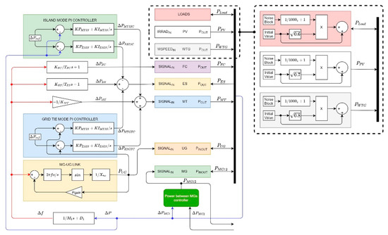
Figure 3.
Schematic of individual MG.

Table 1.
Microgrid parameters, initial and fixed. Reprint with permission [11]; 2019, IEEE.
The precise simulation of MG components dynamics such as MT, FC, and ES, requires high-order mathematical models that consider physical constraints and nonlinearities. However, simplified models are generally employed. In this work, simplified models of the system components in the form of low-order transfer functions were presented. Examples of these transfer functions are Equations (3)–(6) where the dynamic behavior of the device is determined only by a gain and a time constant. Following the work of Li et al. [3], the controller transfer functions that govern the adjustment of the electrical power consumption of the ES , the power generated by the FC , and MT respond to the frequency deviation from nominal values observed in the MG are:
where are ES, FC, and MT proportional gain factors and are the ES and FC time constants.
When connected to UG, the MG PI controllers that govern MT generation and ES demand are set to minimize the amount of power traded with UG and are described by the following equations [8]:
where are control signals for grid-connected ES and MT, are the proportional gains for ES and MT, and are the integral gains of ES and MT. ( is the deviation from the expected value.
When operating in the island mode, The MG PI controllers that govern MT generation and ES demand are set to minimize the generation/demand imbalance and are described by the following equations:
where are control signals for island operation of ES and MT. are the proportional gains for ES and MT. are the integral gains of ES and MT. ( is the power mismatch at the MG bus. From the work of Vachirasricirikul et al. [5], the standard deviation from an initial value and of the solar PV and WTG generation is presented in Figure 3 (insert) and are modeled as:
Similarly, the standard deviation of the load from an initial value is modeled as:
To model , and , a noise block times a first-order low-pass filter is multiplied by the standard deviations of initial values (11–13) as described in Figure 3. The power flow from UG to MG, is:
where is line reactance between MG and UG and obtained from where is 60 Hz and , is the relative phase angle.
Since electrical loads and renewable generation fluctuate randomly, a robust MG controller is necessary to achieve frequency stability throughout the system. In this work we proposed a method to obtain an optimal set of controller parameters for (1) a single MG in stand-alone and UG connected mode, and (2) for two interconnected MGs in the stand-alone and UG connected mode. For a larger system of interconnected MGs and the UG, the method would be similar. In this work, robustness is measured from a practical point of view, for example, after a disturbance, the frequency deviation will return to within the tolerance window. To achieve power balance in the MG, the devices subject to control are ES (controllable load), MT, and FC (controllable generators). Three types of disturbances are considered, MT generator failure, PV generation loss, and MG a sudden increase in MG load. For each case, we implemented a particular objective function. In the results section, for each result, the objective function was described. To minimize the objective functions, in all cases, genetic algorithm was implemented. MATLAB/SIMULINK software was used to implement the models. When dealing with interconnected MGs, one of the MGs may trade power with a nearby MG or with the UG, this condition may lead to an additional optimization layer. Cost minimization (which includes switch operation and power trading) is achieved by distributed decision making, as shown in Figure 2. Each MG controller can import power from the most affordable source and export power to the highest bidder. For this to happen, energy prices (actual and projected) must be communicated between parties in real-time. In the results section, we only proved the frequency stability of the system under topology switching. Using our preliminary work [11] as a starting point, for each MG, a set of initial and fixed parameters is given in Table 1. The initial MG controller parameters are described in Table 2. Optimized parameters are given later in Table 3.
Table 2.
MGC initial parameters. Reprint with permission [11]; 2019, IEEE.
Table 3.
Optimized parameters.
2.2. Model Parameters
2.3. Mechanisms of Energy Trading
One of the main contributions of this work was the analysis of configurable interconnections combined with three different types of power trading mechanisms. Before we explain how each of the trading mechanisms works, we would like to underscore that these mechanisms are based on frequency stability considerations, not from any specific market designs. On the one hand, these mechanisms can be viewed as limiting cases of market designs; and on the other hand, the study of these mechanisms facilitates the exploration of the relations between trading and stability.
2.3.1. Natural Power Trading
We denoted “natural power trading” as the power flowing from one MG to the other when connected directly with a line from one bus to the other. This is modeled by:
where, is the line reactance the tie between MG1 with MG2 and obtained from where is 60 Hz and is the relative phase angle.
2.3.2. Conservative Power Trading
We denoted “conservative power trading” as the trading between interconnected MGs subject to the following rules: (1) If both MGs need power, no trading occurs. (2) If both MGs have excess power, no trading occurs. (3) If MG1 has excess power and MG2 needs power, two things can happen: (3.1) if the power available from MG1 is less than the power need of MG2, then transfer what MG1 has available; (3.2) if the power available from MG1 is more than the power need of MG2, then transfer only what MG2 needs. (4) If MG1 needs power and MG2 has excess power, two things can happen: (4.1) if the power available from MG2 is less than the power need of MG1, then transfer what MG2 has available; (4.2) if the power available from MG2 is more than the power need of MG1, then transfer only what MG1 needs, or mathematically: , is determined by:
where is the power flow between MGs under conservative power trading, is the power deviation in MG1 bus, and is the power deviation in the MG2 bus.
2.3.3. Active Power Trading
In “active power trading”, trading is allowed only under certain circumstances. For this paper we set the following restrictions: (1) If both MGs are operating with their within the established safety threshold of ± 0.5 Hz no trading occurs. (2) If any or both MGs are operating with their between (−0.05 and −0.1 Hz) or (0.05 and 0.1 Hz), trading occurs following the method explained in Equation (15). (3) If one or both MGs are operating with beyond , no trading occurs. Therefore, , is determined by:
where is the power flow between MGs under active power trading. and are the frequency deviations from the nominal value at the MG1 and MG2 buses respectively. In active power trading, more power support can be requested compared to conservative trading, but only to a limit that prevents cascade failure under large disturbances.
3. Results
This section provides representative results that show the robustness of individual MGs (both island and grid-connected modes) and interconnected MGs, the effects of energy transactions on operational costs, and the optimal interconnection strategies for multi-MG systems.
3.1. Robustness of Individual Microgrids
Figure 4, Figure 5, Figure 6 and Figure 7 show the optimization convergence and frequency deviation of a single MG in the grid-connected mode. The objective function (to minimize) is defined as , where is s and is s. describes the average of the absolute value of the frequency deviation from the nominal value during the studied time interval . Since these cases are grid-connected scenarios, only the grid-connected PI controller parameters are optimized. Optimized parameters can be seen in Table 3. All cases are analyzed from the perspective of MG1. Figure 4a shows the optimization convergence process of and Figure 4b the optimized frequency deviation of MG1 in normal operation with no disturbances applied. Since the MG is connected to UG, the frequency deviation is minimal. For the following cases, we considered three types of local disturbances within the MG. In Figure 5, the PV generation failed (instantaneous PV plant shut down) at s. This disturbance produced a frequency sag; however, the decline was within the frequency threshold. In Figure 6, at s, MG1 was subject to a sudden load increase (40 kW in 2 s). This disturbance produced a frequency sag and a subsequent spike, both within the threshold boundaries. In Figure 7, at s, the MT lost power by 70 kW in 20 s. This disturbance was barely noticeable mainly due to the relatively long term (20 s) development. We could conclude, for all cases (Figure 4, Figure 5, Figure 6 and Figure 7), as long as MG1 was connected to the UG (and by default, there were no restrictions on the power flow between MG1 and UG), the frequency deviation was minimal (within Hz range). In figure captions, the symbol ⇔ was used to denote “connected” and the symbol ⇎ was used to denote “disconnected”.
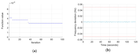
Figure 4.
Optimization convergence and frequency deviation of a single MG in grid-connected mode. Case 1: MG1⇔UG. No disturbances are applied, this case is considered normal operation. (a) Optimization of the controller parameters convergence process. (b) Frequency deviation of the optimized solution. Red dotted lines show the ± 0.05 Hz threshold. Under this scenario, frequency fluctuations are minimal compared to all other cases.
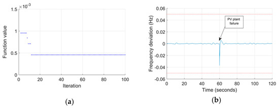
Figure 5.
Optimization convergence and frequency deviation of a single MG in the grid-connected mode. Case 2: MG1⇔UG. At t = 60 s photovoltaic (PV) plant failure. (a) Optimization of controller parameters convergence process. (b) Frequency deviation of the optimized solution. Red dotted lines show ± 0.05 Hz threshold. Even when subject to the failure of the MG PV plant, while connected to UG, frequency stability remains within the desired threshold.
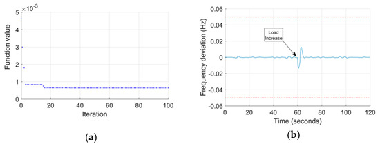
Figure 6.
Optimization convergence and frequency deviation of a single MG in the grid-connected mode. Case 3: MG1⇔UG. At t = 60 s load increase (40 kW in 2 s). (a) Optimization of controller parameters convergence process. (b) Frequency deviation of the optimized solution. Red dotted lines show ± 0.05 Hz threshold. Similar to the previous result, when connected to UG, frequency stability remains within the threshold.
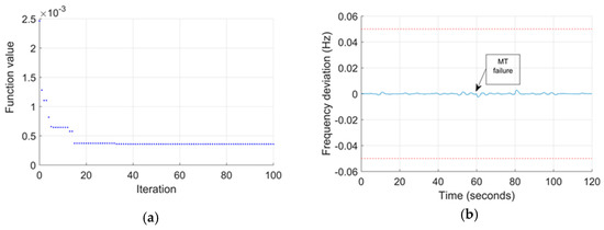
Figure 7.
Optimization convergence and frequency deviation of a single MG in the grid-connected mode. Case 4: MG1⇔UG. At t = 60 s microturbine (MT) loses power (70 kW in 20 s). (a) Optimization of controller parameters convergence process. (b) Frequency deviation with the best solution. Red dotted lines show the ± 0.05 Hz threshold. Similar to the previous result, when connected to UG, frequency stability remains within the threshold.
Figure 8, Figure 9, Figure 10 and Figure 11 show the optimization convergence process and frequency deviation of a single MG in the island mode. Here we wanted to tune the island mode controller parameters to minimize frequency deviation. The objective function is as described earlier. Since these were island mode cases, the PI controller parameters to be optimized were for the island mode PI controller as seen in Figure 3. Optimized parameters for all cases can be seen in Table 3. All the tests are presented from the perspective of MG1. Figure 8 shows the optimization results and frequency deviation of MG1 in normal operation with no disturbances applied. Comparing Figure 8 (island mode) with Figure 4 (grid-connected), it is obvious that was more significant in the island mode than in the grid-connected mode; both it is still well within the tolerance threshold. In Figure 9, at s, a disturbance was applied (instantaneous PV plant shut down). This event prompted a frequency deviation beyond the tolerance level for approximately one second. The same disturbance did not breach the threshold in grid-connected mode. In Figure 10, at s, the load increased by 40 kW in a 2 s ramp. This disturbance produced an out of tolerance effect on the MG frequency, which was extended for about 6 s. In Figure 11, at s, the MT lost power by 70 kW in 20 s. We could conclude, in all cases (Figure 8, Figure 9, Figure 10 and Figure 11), disturbances could have a temporary detrimental effect on frequency stability. However, shortly after the disturbances, the frequency stabilizes without the support from external sources such as the UG of a neighboring MG.
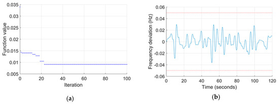
Figure 8.
Optimization convergence process and frequency deviation of a single MG in the island mode. Case 5: islanded MG1. No disturbances are applied. (a) Optimization convergence process. (b) Frequency deviation. Red dotted lines show the ± 0.05 Hz threshold. As expected, when islanding, a single MG suffers an increased frequency deviation from the nominal value.
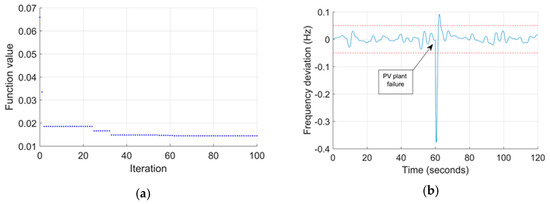
Figure 9.
Optimization convergence process and frequency deviation of a single MG in the island mode. Case 6: islanded MG1. At t = 60 s PV plant failure. (a) Optimization convergence process. (b) Frequency deviation. Red dotted lines show the ± 0.05 Hz threshold. The same failure as in Figure 5 produces a frequency sag outside of the desired threshold. However, the system returns to the desired range in a short time. Figure 10 and Figure 11 show similar behavior.
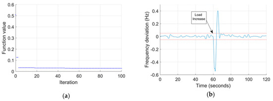
Figure 10.
Optimization convergence process and frequency deviation of a single MG in the island mode. Case 7: islanded MG1. At t = 60 s load increase (40 kW in 2 s). (a) Optimization convergence process. (b) Frequency deviation. Red dotted lines show the ± 0.05 Hz threshold.
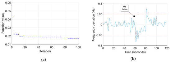
Figure 11.
Optimization convergence process and frequency deviation of a single MG in the island mode. Case 8: islanded MG1. At t = 60 s MT loses power (70 kW in 20 s). (a) Optimization convergence process. (b) Frequency deviation. Red dotted lines show the ± 0.05 Hz threshold.
Above, we optimized the MG controller parameters for each case and plotted the frequency fluctuations under optimized parameter settings. To tune the controller for applications, it is necessary to find an optimal set of parameters that work well in different disturbance scenarios. The objective function can be defined as (minimize) where represents the likelihood (weight) of the i-th scenario and is the average absolute frequency deviation in the scenario. Now we chose , , and , where respectively stand for the weight factors of PV loss, load increase, and MT failure likelihood of the scenario. The results of this approach are shown in Figure 12a single set of controller parameters was applied for all cases. The analyzed scenario was for an islanded MG. Figure 12a shows the optimization convergence process. Figure 12b,c were very close to Figure 9b and Figure 10b (the first two scenarios), while the results in Figure 12d was not as good as Figure 11 due to the low weight assigned.
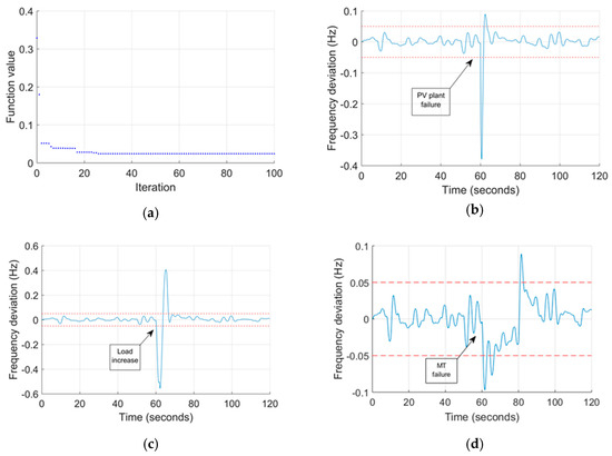
Figure 12.
Case 9: (a) Optimization convergence process. (b) Frequency deviation, at t = 60 s PV pant failure. (c) Frequency deviation, at t = 60 s load increase (40 kW in 2 s) (d) Frequency deviation, at t = 60 s MT loses power (70 kW in 20 s). Results suggest that a single set of controller parameters will not provide successful frequency deviation damping for all analyzed cases.
In Figure 13, we implement a similar approach as in the case presented in Figure 12. However, an alternative objective function was used: (minimize) where is the time (in seconds) that the frequency stays outside the defined range in the i-th scenario. The results were similar to Figure 12. For simplicity, we used the objective function in Figure 12 hereafter.
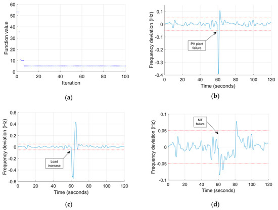
Figure 13.
Case 10: (a) Optimization convergence process. (b) Frequency deviation, at t = 60 s PV plant failure (full power instantaneous). (c) Frequency deviation, at t = 60 load increase (40 kW in 2 s). (d) Frequency deviation, at t = 60 s MT loses power (70 kW in 20 s). Results from this case analysis (in which another objective function is used compared to Figure 12) are similar to the ones observed in Figure 12.
3.2. Robustness of the Inter-Connected Two-Microgrid System
In all the simulated scenarios above, the optimized MGC could maintain grid-connected and islanded MG frequency stability to a satisfactory level. However, in the island mode, temporary breaches of frequency threshold could be observed, always returning to a stable operation after the disturbance was cleared. Now with the controller design validated, we analyzed the impact of interconnecting adjacent MGs on frequency stability. We tested the three types of power trading as described in the methodology section. In Figure 14, two adjacent MGs were connected while both disconnected from UG. We sought to optimize the island mode controller parameters in both MGs. The objective function is (minimize) where corresponds to each of the interconnected MGs and therefore, is the average absolute value of frequency deviation on each of the interconnected MG. For the simulation, is s and is s. describes the average of the absolute value of the frequency deviation from the nominal value during the studied time interval . In Figure 14, the two adjacent MGs were initially disconnected from each other. At , they became connected. The trading mechanism established for this case was natural power trading as defined before. In Figure 14a the optimization convergence process is presented. In Figure 14b, once the MGs were connected, their frequency deviations converged. In Figure 14c, at , the PV plant in MG2 failed. The impact on of this disturbance was larger on MG2 but it was also transferred to MG1. At , MG1 load increased 40 kW in 2 s. The impact of the disturbance on was now greater in MG1. In both cases, the frequency deviation could fall outside of the threshold but the magnitude was smaller than those observed on a single islanded MG (as in Figure 13b,c), demonstrating that interconnected MGs had increased resiliency to disturbances. In Figure 14d, a large load increase was observed in MG2 at (120 kW in 4 s). This disturbance exceeded the generation capacity of MG2 and made MG1′s MT and ES reach the maximum and minimum limits. Evidently, natural power trading could lead to the collapse of both MGs, because there was no mechanism to limit the destabilizing disturbance transmission between them.
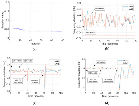
Figure 14.
Frequency deviations under natural power trading (Case 11). (a) Optimization convergence process. (b) At t = 20 s MG1⇔MG2. No further perturbances. (c) At t = 20 s MG1⇔MG2. At t = 40 s MG2 PV plant failure. At t = 80 s MG1 Load Increase (40 kW in 2 s). (d) At t = 20 s MG1⇔MG2. At t = 40 s MG1 PV power plant failure. At t = 80 s MG2 large load increase (120 kW in 4 s). Characteristics: When MGs are interconnected, they tend to support each other, and system stability is improved. However, large disturbances can cause the collapse of both MGs.
To reduce the “negative impact” propagation among interconnected MGs, we tested two alternative power trading methods. In Figure 15 we implemented conservative power trading. In Figure 15b, the interconnected MGs were trading. In contrast with natural power trading shown in Figure 14b, the frequencies in each MG remained independent. In Figure 15c, MG1 frequency deviation was compared between no-trading (islanding) and conservative-trading cases. In both cases, a 40 kW load increase in 2 s was applied. The stabilization effect of the trading method on frequency was not much improved since the capacity of MGs supporting each other was limited. However, conservative trading could prevent a disturbance cascade between MGs. In Figure 15c, we used the controller parameters for MG1 and MG2 obtained from single islanded MG optimization (e.g., Figure 12). In Figure 15d, we compared the trading case of Figure 15c with the case in which the two MG controllers’ parameters were jointly optimized (using the Figure 15c parameters as initial values). The optimization convergence process is shown in Figure 15a. The frequency deviation was substantially reduced.
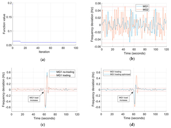
Figure 15.
Frequency deviations under conservative power trading (Case 12). (a) Optimization convergence process. (b) Two MGs trading based on surplus or deficit at each MG’s main bus. No disturbances. (c) Orange line: At t = 60 s load increase in MG1 (40 kW in 2 s). No trading case (islanding). Blue line: MG1 trading with MG2. At t = 60 s, load increase in MG1 (40 kW in 2 s), MG2 MT increase power (40 kW in 2 s). (d) Same case as Figure 15c but with optimized parameters.
As an intermediate mechanism between “natural power trading” and “conservative power trading”, the “active power trading” was as follows: power trading was allowed when frequency deviation was between 0.051 to 0.1 Hz and −0.1 to −0.051 Hz and no trading between −0.05 and 0.05 Hz. In Figure 16b, as long as both MGs remained within this frequency deviation threshold, they remained independent. In Figure 16c, we applied a large disturbance in MG1 (80 kW in 2 s) this additional load exceeded the MT and ES controlling capacity. The orange line shows the frequency deviation of MG1 under the conservative trading method, leading to the MG1 collapse. The blue line shows the effect of the active trading method where despite large transient sag, the frequency returns to be within the safety threshold. In Figure 16d, we compared the blue line of Figure 16c with the case in which the two MG controllers’ parameters were jointly optimized (using the Figure 16c parameters as initial values) and observed an additional reduction of frequency deviation. It has been shown that this method could transfer power between interconnected MGs up to a limit that was higher than conservative trading. If the disturbance is too large and one of the MGs is likely to collapse, the other will support up to a certain point and then disengage (unlike natural trading). The optimized parameters for all the above cases (1 through 13) are listed in Table 3 below.
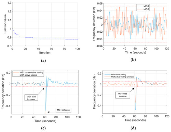
Figure 16.
Frequency deviations under active power trading (Case 13; trading on-demand with limitation). (a) Optimization convergence process. (b) MGs in normal operation. No disturbances. (c) Blue line: Active trading case. At t = 60 s load increase in MG1 (80 kW in 2 s). Orange line: Conservative trading case. At t = 60 s load increase in MG1 (80 kW in 2 s) no scheduled support from MG2. (d) Same case as Figure 16c except the active trading parameters are optimized.
In Figure 17, we present some results from the perspective of power flow. Figure 17a shows the power output of MTs in both MGs with no disturbances applied. Figure 17b shows the power flow between MG1 and MG2 under “natural power trading” with no disturbance (blue line) and disturbance case (at t = 400, 40 kW in 2 s load increase in MG1). Large power flow was observed from MG2 to MG1. In Figure 17c, the disturbance case (orange line) of Figure 17c was compared to the same case under the active trading mechanism. The power transfer between MGs was clearly affected by the trading mechanism, which subsequently also affected the frequency stability of the interconnected system.
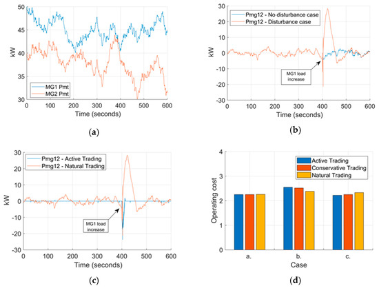
Figure 17.
(a) MT power generation in MG1 and MG2. No disturbance conditions. (b) Power flow between MG1 and MG2. Blue line: no disturbance. Orange line: At t = 400 s, load increase in MG1 (40 kW in 2 s). (c) Power flow between MG1 and MG2. Blue line: active trading; orange line: natural trading. (d) Cost comparisons: a. No disturbances b. At t = 400 s, load increase in MG1 (40 kW in 2 s). c. At t = 400 s, load increase in MG2 (40 kW in 2 s).
3.3. Effects of Energy Transactions on Operational Costs
In Figure 17d, still with both MGs disconnected from UG, we calculated the kWh cost for the simulation period (10 min). The operational cost calculation was performed (time omitted) by:
where is the operational cost of MG1. is the cost of generating 1 kWh using MG1 MT. is the cost of buying 1 kWh from the UG. is the cost of buying 1 kWh from MG2. is the income obtained from selling 1 kWh to the UG. is the income obtained from selling 1 kWh to MG2. In the absence of disturbances, the three mechanisms have the same cost performance. In the case of load increase in MG1, the operating cost of MG1 was highest under active trading, because a net import of power from MG2 was dominant (Figure 17c). Similarly, in the case of a load increase in MG2, the operating cost of MG1 was lowest under active trading.
Next, we analyzed how the different interconnections between MGs and UG could affect operational costs. The main objective in this section was to show that switching interconnection configuration could lead to an optimized operation cost. The operational cost calculation was performed only from the perspective of MG1. Natural power trading was selected as the interconnection method between MGs, this was due to the larger amount of traded energy between MGs, which allowed more evident results. Two cases were analyzed in Figure 18. For case a, we assumed the following: (1) the kWh unit price for buying and selling from UG = 1, (2) the kWh unit price for buying and selling from a neighbor MG = 0.8, and (3) the cost of producing 1 kWh with the MT is 0.5. No disturbances were applied to this case. For case b, we assumed that the kWh unit price for buying and selling from UG = 1.5. In both cases, a 40 kW load increase (in 2 s) was applied at t = 60 s and the simulation time was 120 s. In Figure 18, one could see that depending on the UG electricity price and the real-time multi-MG system operational characteristics, it was possible to change the interconnection configuration to reduce operating costs.
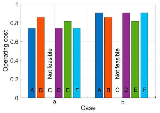
Figure 18.
Operational costs of MG1 under difference interconnection configurations: (A) = MG1⇔UG⇔MG2⇔MG1; (B) = MG1⇎UG⇔MG2⇔MG1; (C) = MG1⇎UG⇎MG2⇎MG1; (D) = MG1⇔UG⇔MG2⇎MG1; (E) = MG1⇎UG⇎MG2⇔MG1; and (F) = MG1⇔UG⇎MG2⇔MG1. Scenario (a). MG1 Operating cost under different interconnection configurations. Scenario (b). MG1 Operating cost under different interconnection configurations with UG kWh price increased by 50%. In (a,b), at t = 60 s, load increases in MG1 (40 kW in 2 s).
3.4. Optimal Interconnection Strategies for System Operation
To illustrate the findings in the previous subsection, we implemented an example (Figure 19) based on the conditions established for Figure 18 case b. Assuming an increase of the energy price signal from 1 to 1.5 (Figure 19a), a tradeoff between power quality and costs could be observed. When connected to UG and MG2 (case b-A) the operation cost will naturally go up. If the interconnection was switched from case b-A to case b-E, an operational cost reduction could be achieved (Figure 19c), while frequency deviation became more significant (Figure 19b).
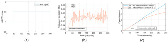
Figure 19.
(a) UG price signal at t = 50 s increases from 1 to 1.5. (b) Frequency deviation. The blue line shows the frequency deviation under MG1⇔UG⇔MG2⇔MG1. The orange line shows frequency deviation when at t = 50 s, MG1 switches configuration to MG1⇎UG⇎MG2⇔MG1 and performs active trading. (c) The operational cost dynamics.
4. Conclusions
This work developed the simulation model of a multi-MG system, which included several distributed generation resources, loads, a controllable power generator (microturbine), and a controllable load (electrolyzer). Various interconnection configurations of the MGs and the UG were considered. Using MATLAB/SIMULINK and genetic algorithm, we optimized the controller parameters to minimize frequency deviation when the MGs were in island mode. In the grid-connected mode, the frequency stability was guaranteed for a wide range of parameters; in the island mode and under disturbances, the frequency deviation needs to be reduced to be within ± 0.05 Hz with optimized controller parameters. Different definitions of objective functions were compared and in this work, we used the averaged absolute frequency deviation during the simulation period.
The frequency stability of a system of interconnected MGs that are all disconnected from the UG was then studied. In the case of two MGs, we demonstrated three different interactions between MGs: natural trading, conservative trading, and active trading. The main findings included: (a) the natural trading was the simplest but might cause cascading failures under large disturbances; (b) the conservative trading could prevent cascading failure but often fell short of power support among neighboring MGs; (c) the active trading overcame the disadvantages of conservative trading by allowing power transfer up to a limit set by frequency stability requirement; and (d) in the latter two mechanisms, the joint optimization of the parameters of the controllers of the MGs could result in an additional reduction of frequency deviation.
Next, we investigated the operational cost performance of different combinations of trading mechanisms and interconnection configurations. Given the UG price signals and the multi-MG system operational characteristics, the costs incurred in each MG could be reduced by switching interconnection configurations or using different trading mechanisms. However, it is shown that there was a trade-off between cost minimization and frequency stability, and cost reductions could sacrifice frequency stability in some cases.
This work presented substantial developments in the understanding of the multi-MG systems by investigating the relations among frequency stability, operational costs, trading mechanisms, and interconnection configurations. It filled a gap in the previous studies that either only implement stability/cost control in fixed configurations or design trading mechanisms without stability considerations. The modeling framework and methodology demonstrated in this work will be instrumental to inform the future planning, operation strategy making, and controller design of multi-MG systems to make them more robust, resilient, and meanwhile, cost-effective.
Author Contributions
M.L and X.Z designed the research; M.L. performed the model validation and analyzed the data; M.L. wrote the original draft; X.Z. reviewed and edited the draft. Both authors have read and agreed to the published version of the manuscript. All authors have read and agreed to the published version of the manuscript.
Funding
This research received no external funding.
Conflicts of Interest
The authors declare no conflict of interest.
References
- Lainfiesta-Herrera, M.; Zhang, X.; Wu, J.; Song, H. Developing a Decision Support System for the Optimal Operating Strategies of a Polygeneration Facility. In Proceedings of the 2019 IEEE Innovative Smart Grid Technologies-Asia (ISGT Asia), Chengdu, China, 21–24 May 2019; pp. 1199–1204. [Google Scholar]
- Kaur, A.; Kaushal, J.; Basak, P. A review on microgrid central controller. Renew. Sustain. Energy Rev. 2016, 55, 338–345. [Google Scholar] [CrossRef]
- Li, X.; Song, Y.-J.; Han, S.-B. Frequency control in micro-grid power system combined with electrolyzer system and fuzzy PI controller. J. Power Sources 2008, 180, 468–475. [Google Scholar] [CrossRef]
- Bevrani, H.; Francois, B.; Ise, T. Microgrid Dynamics and Control; John Wiley & Sons: Hoboken, NJ, USA, 2017; ISBN 978-1-119-26370-8. [Google Scholar]
- Vachirasricirikul, S.; Ngamroo, I.; Kaitwanidvilai, S. Application of electrolyzer system to enhance frequency stabilization effect of microturbine in a microgrid system. Int. J. Hydrog. Energy 2009, 34, 7131–7142. [Google Scholar] [CrossRef]
- Lopes, J.A.P.; Moreira, C.; Madureira, A.G. Defining Control Strategies for MicroGrids Islanded Operation. IEEE Trans. Power Syst. 2006, 21, 916–924. [Google Scholar] [CrossRef]
- Elrayyah, A.; Cingoz, F.; Sozer, Y.; Anwar, S. Construction of Nonlinear Droop Relations to Optimize Islanded Microgrid Operations. IEEE Trans. Ind. Appl. 2015, 51, 1. [Google Scholar] [CrossRef]
- Hua, H.; Hao, C.; Qin, Y.; Cao, J. A Class of Control Strategies for Energy Internet Considering System Robustness and Operation Cost Optimization. Energies 2018, 11, 1593. [Google Scholar] [CrossRef]
- Hao, C.; Hua, H.; Qin, Y.; Cao, J. A Class of Optimal and Robust Controller Design for Energy Routers in Energy Internet. In Proceedings of the 2018 IEEE International Conference on Smart Energy Grid Engineering (SEGE), Oshawa, ON, Canada, 12–15 August 2018; pp. 14–19. [Google Scholar]
- Jadhav, A.M.; Patne, N.R.; Guerrero, J.M. A Novel Approach to Neighborhood Fair Energy Trading in a Distribution Network of Multiple Microgrid Clusters. IEEE Trans. Ind. Electron. 2018, 66, 1520–1531. [Google Scholar] [CrossRef]
- Lainfiesta-Herrera, M.; Subramanyam, S.A.; Zhang, X. Robust Control and Optimal Operation of Multiple Microgrids with Configurable Interconnections. In Proceedings of the 2019 IEEE Green Technologies Conference (GreenTech), Lafayette, LA, USA, 3–6 April 2019; pp. 1–4. [Google Scholar]
- Hussain, A.; Kim, H.-M.; Kim, H.-M. A Resilient and Privacy-Preserving Energy Management Strategy for Networked Microgrids. IEEE Trans. Smart Grid 2016, 9, 2127–2139. [Google Scholar] [CrossRef]
- Park, S.; Lee, J.; Bae, S.; Hwang, G.; Choi, J.K. Contribution-Based Energy-Trading Mechanism in Microgrids for Future Smart Grid: A Game Theoretic Approach. IEEE Trans. Ind. Electron. 2016, 63, 4255–4265. [Google Scholar] [CrossRef]
- Wang, Z.; Chen, B.; Wang, J.; Begović, M.; Chen, C. Coordinated energy management of networked Microgrids in distribution systems. IEEE Trans. Smart Grid 2015, 6, 45–53. [Google Scholar] [CrossRef]
- Wu, J.; Guan, X. Coordinated Multi-Microgrids Optimal Control Algorithm for Smart Distribution Management System. IEEE Trans. Smart Grid 2013, 4, 2174–2181. [Google Scholar] [CrossRef]
- Kou, P.; Liang, D.; Gao, L. Distributed EMPC of multiple microgrids for coordinated stochastic energy management. Appl. Energy 2017, 185, 939–952. [Google Scholar] [CrossRef]
- Gregoratti, D.; Matamoros, J. Distributed Energy Trading: The Multiple-Microgrid Case. IEEE Trans. Ind. Electron. 2014, 62, 2551–2559. [Google Scholar] [CrossRef]
- Zhao, B.; Wang, X.; Lin, D.; Calvin, M.M.; Morgan, J.C.; Qin, R.; Wang, C. Energy Management of Multiple Microgrids Based on a System of Systems Architecture. IEEE Trans. Power Syst. 2018, 33, 6410–6421. [Google Scholar] [CrossRef]
- Wang, H.; Huang, J. Incentivizing Energy Trading for Interconnected Microgrids. IEEE Trans. Smart Grid 2016, 9, 2647–2657. [Google Scholar] [CrossRef]
- Bullich-Massagué, E.; Diaz-Gonzalez, F.; Aragues-Penalba, M.; Girbau-Llistuella, F.; Olivella-Rosell, P.; Sumper, A. Microgrid clustering architectures. Appl. Energy 2018, 212, 340–361. [Google Scholar] [CrossRef]
- Gazijahani, F.S.; Ravadanegh, S.N.; Salehi, J. Stochastic multi-objective model for optimal energy exchange optimization of networked microgrids with presence of renewable generation under risk-based strategies. ISA Trans. 2018, 73, 100–111. [Google Scholar] [CrossRef] [PubMed]
- Arefifar, S.A.; Ordonez, M.; Mohamed, Y. Energy management in multi-microgrid systems—Development and assessment. In Proceedings of the 2017 IEEE Power Energy Society General Meeting, Chicago, IL, USA, 16–20 July 2017; pp. 1–5. [Google Scholar]


© 2020 by the authors. Licensee MDPI, Basel, Switzerland. This article is an open access article distributed under the terms and conditions of the Creative Commons Attribution (CC BY) license (http://creativecommons.org/licenses/by/4.0/).