1. Introduction
A number of engineering applications require estimation of radiation exchange between surfaces which in turn leads to computation of ‘view factor’. View factor (VF), F
i-j may be defined as the fraction of the radiation leaving surface i that is intercepted by surface j [
1].
The view factor (VF) is also known in engineering literature as geometry-, angle-, shape- or configuration factor. This article will be based on obtaining numerical solution for view factor using four procedures. The procedures range from the simplest routine that uses a uniform grid (brute force approach) to a procedure that efficiently combines the Monte-Carlo technique with generation of a non-uniform grid that increases the cell size as one draws away from the emitter–receiver common edge. The manner in which the non-uniform grid is generated has been refined after trialling very many procedures.
A number of engineering applications of the present work are also identified in the present article.
2. Case Study Description
Attention is drawn towards
Figure 1 and
Figure 2 which demonstrate some of commonly encountered applications of the present work.
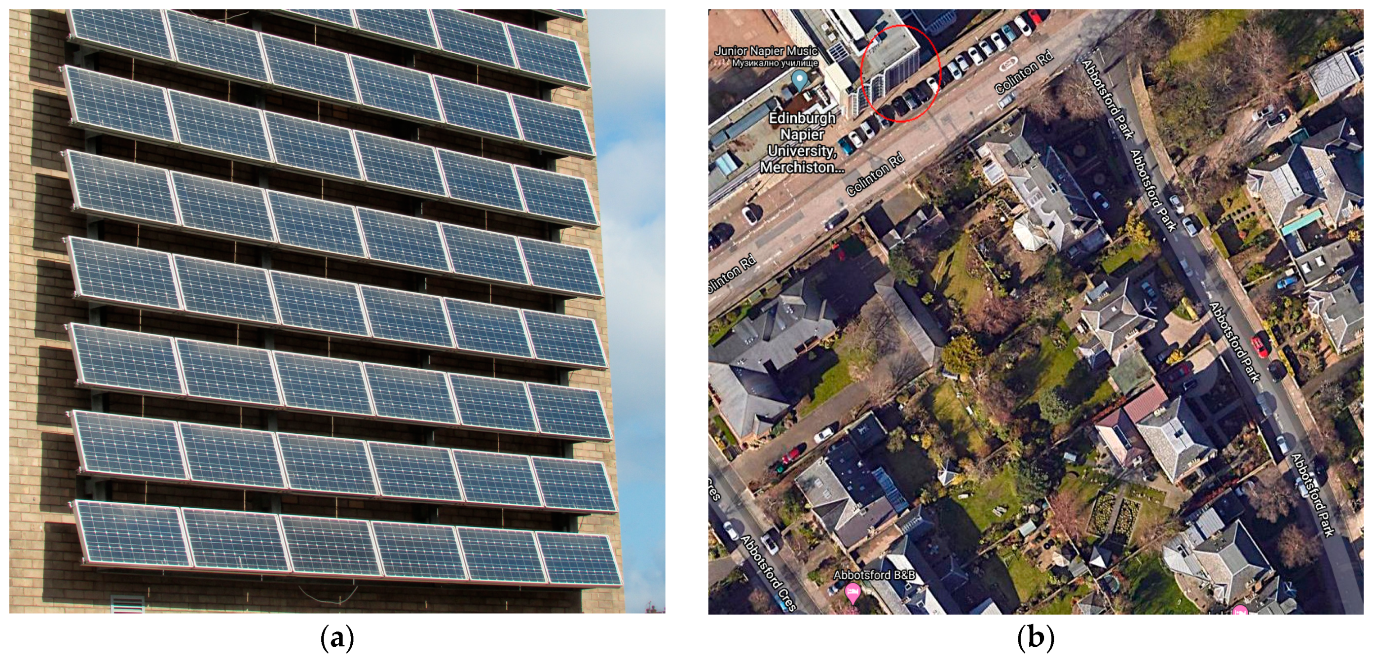
Figure 1 shows the influence that thermal radiation heat transfer has in determining the surface temperature due to overnight cooling. Two automobiles that were parked adjacent to each other may have widely different windshield temperatures purely as a result of the surfaces they have in their view. The convective heat loss is the same for the two windshields as are the view factors. However, the car shown in
Figure 1a achieved a much lower surface temperature owing to its radiation emission to a clear sky. The other windshield of
Figure 1b exchanges thermal radiation, mostly with building surfaces which are much warmer and hence does not show any trace of frost.
Figure 2 shows some aspects of Edinburgh Napier University Building-Integrated Photovoltaic (BIPV) installation. The PV modules face south-east and are inclined at an angle of 75° from the horizontal. The foreground view is shown in part (b) of
Figure 2. As would be expected of an urban setting the foreground is non-uniform and is composed of surfaces with widely different reflectivity. In winter, in particular, the rooftops of the foreground houses are covered with snow which offers a high reflectance. In summer, autumn, and spring the grass and tree tops offer different reflectance. Reference [
2] provides more details of the above facility.
The total incident radiation on a surface such as a PV panel or a solar thermal collector (vertical or inclined) is the sum of beam, sky-diffuse, and ground reflected radiation from various surfaces. It is the latter component that is the subject of this article.
The solar water heating technology has matured over the past several decades. However, the Building Integrated Photovoltaic [BIPV and PV farms have only recently seen a sharp rise in their installations. Furthermore, recent articles have emerged that show the potential of large irradiation gains that may be made by deploying highly reflective surfaces in the foreground of PV modules. Furthermore, the recent advent of bifacial PV modules has brought to attention the importance of ground-reflected radiation. In such a module the PV cells are mounted on both sides of the module, the back side receiving only radiation that is reflected off the ground. The back-side of the PV module has a much higher view factor and hence its estimation gains further importance.
Within the past two decades the cell phone has become an essential tool for communication. The microwave radiation effects of a cell phone may be classified as thermal and non-thermal. The work of Girish Kumar [
3] has shown that the above non-thermal effects are several times more harmful than thermal effects. One way to measure the effect of microwave radiation from cell phones is in terms of Specific Absorption Rate (SAR) which is expressed in W/kg. In the US, the SAR limit for cell phones is 1.6 W/kg. It has therefore been recommended that a cell phone should not be used for more than 18 to 24 min a day. One cell phone manufacturer has also recommended that the device should be kept at least 25 mm from the human body. Note that for any scenario study for the use of cell phone view factor between the emitter (cell phone) and human head (receiver) would be required and this would depend on the distance at which the device is held by its user.
In the present article, we present efficient routines for view factor analysis taking into account the non-homogeneous nature of the foreground that may offer a range of varying reflectance.
3. Procedure for Obtaining View Factor between Two Plane, Inclined Surfaces
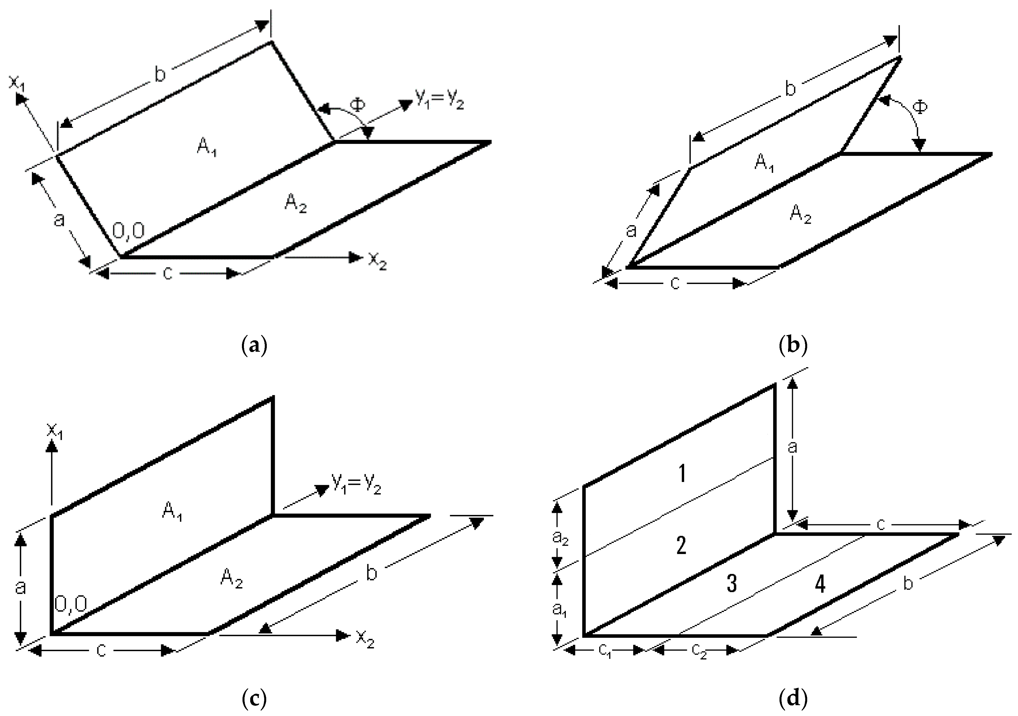
For any two elemental surfaces such as those shown in
Figure 3, F
1-2 is given as Equation (1):
where
R1-2 is the distance between both differential elements
dA1 and
dA2;
A1 and
A2 are the area of the two surfaces; and
Φ1 and
Φ2 are the angles between the normal vectors to both differential elements and the line between their centres.
See
Figure 4. If we apply Equation (1) to two rectangular surfaces
A1 with dimensions
a ×
b and
A2 with dimensions
c ×
b, with angle
Φ between them, then
β = π − ϕ,
and
and
The resulting integral is Equation (2):
The solution of this integral is Equation (3), where
,
,
, and
[
4].
Thus, Equation (3) still remains unresolved analytically as its very end part requires further integration. The view factor F1-2 can be estimated partially analytically, partially numerically.
In a previous work [
4], the present authors presented a numerical solution of Equation (2) that enables estimation of view factor for geometries such as those shown in
Figure 5.
Furthermore, a Microsoft Visual Basic for Application (VBA) code was developed that enables the user to obtain the view factor for any geometry and reflectivities for the foreground (surface A2).
If we consider the rectangular surfaces
Ai and
Aj with a common edge
b as composed of many very small rectangular areas (
Figure 5a), numeric integration could be used to solve it where
Na,
Nb; and
Nc,
Nd are cell numbers for the receiving and emitting surfaces. The finite increments Δ
a through to Δ
d are defined thus: Δ
u = u/Nu, where
u may take the value of
a,
b,
c, or
d. Further details are provided in Reference [
4].
In the case of a receiving surface such as a solar thermal or PV module being irradiated by a field containing patches of differing reflectance (see
Figure 5), Equation (4) transforms to Equation (5) thus:
4. Previous Work
This section shall present a brief survey of recent methods to obtain view factor. Towards the end of this section the novelty of present work is highlighted.
One of the most authoritative references on the subject of determining view factor is the text due to Siegel and Howell [
5]. Furthermore, Howell [
6] has provided a compendium of formulations for a range of geometries for obtaining view factor.
In the recent past, Gupta at al [
7] have provided a brief review of methods for evaluation of view factor.
Dirsken et al. [
8] have obtained Sky View Factor (SVF) for urban, meadows, and forests in their study of impact of SVF resolution on an Urban Heat Island.
Zhang et al. [
9] undertook a validation study on the positive correlation between SVF and temperature level in vegetation environments and the negative correlation in built-up areas. Their work was based on measurements obtained from 18 sites.
He et al. [
10] provide a detailed account of setting up the Monte Carlo method for obtaining view factor for complex geometries. It is of relevance to note that they have used a million number of rays to obtain the view factor between a finite-length cylinder and a rectangle with two edges that were parallel to cylinder axis and of length equal to that of the cylinder.
Sonmez et al. [
11] used a ray-casting technique to obtain view factor that may have applications within the solar energy sector such as PV cells. An interesting result presented in their work that has a parallel to the present work is the relationship between the estimation error for view factor and the number of rays.
Ivanova and Muneer [
12] extended their numerical view factor solution work [
4] to cover parallel surfaces. Note that in most building energy simulation work you need to obtain view factor for perpendicular, inclined, and parallel surfaces and, thus, references [
4,
12] provide the required solutions. In the remainder of this section a brief review of computer-based procedures for view factor analyses are presented.
The FACET computer code [
13] uses area and contour integration for a range of geometries. The VIEW program [
14] uses interactive graphics for obtaining view factor while the MONTE routine uses a Monte Carlo procedure [
15].
GLAM enables calculation of view factor for axis symmetric geometries [
16] while CNVUFAC [
17] uses a computer-graphics analogue of the unit sphere method.
Alciatore et al. [
18] attempted a closed-form solution of the general three dimensional radiation configuration factor problem using a microcomputer. Jensen [
19] has provided a routine for view factor analysis within the TRNSYS software system. ‘TRNSYS’ stands for Transient Simulation Software.
Emery et al. [
20] have provided a comparative study of methods for comparing the diffuse radiation view factors.
Another authoritative reference on the subject of determining view factor is the book “Engineering Heat Transfer” of Suryanarayana [
21].
Vujicic et al. [
22] have investigated the Monte Carlo method combined with the finite-element (FE) approach for the estimation of view factors in case of uniform emitting or reflectance. Their approach used random points inside the triangular finite elements of the emitting and receiving surfaces.
There are a number of generic procedures that may be used for obtaining view factor some of which are enumerated below. Note that only those methods which have direct bearing on the present work are explained in further detail. Details of other procedures that are enumerated here but not explained further may be obtained from Reference [
4].
- (a)
Direct integration method which attempts to use a numerical solution of Equation (1);
- (b)
Unit sphere method;
- (c)
Ray casting method;
- (d)
Cross string method;
- (e)
Algebraic rule and matrix formulation method; and
- (f)
Monte Carlo Method.
Method (a) is the subject of the present article and therefore explained via Equations (1)–(5). The novelty of the present work is that it provides numerical solution to view factor computation by hybridization of integration method by exploring brute force, Monte-Carlo, and an innovative approach in which non-uniform grid is used. The algorithm to generate the non-uniform grid has been discussed at length.
5. Presently Developed View Factor Routines
This method yields our first of four routines and shall henceforth be called Uniform Populous Grid (UPG) owing to the large number of cells that are generated in this procedure. It obviously is the slowest routine to yield results.
We have also developed a hybrid version of Monte Carlo method within the present work and shall therefore be explained furthermore.
The Monte Carlo (MC) method (Method (f) in the above list) uses repeated random sampling to make numerical estimations of unknown parameters. It enables modeling of complex systems where random variables interact. There are very many applications of Monte Carlo methods though they all rely on random number generation to solve deterministic problems. MCs take their name from the famous casinos located in the city of Monte Carlo.
In the traditional version, MCs are used purely as a statistical technique. In the present context, though, a hybrid integration-MC method has been used which is explained thus. We use MC to select cells at a random, i.e., if 10% of the cells are to be used for obtaining the view factor for infinitesimal cells then only those cells that result from obtaining numbers between zero and 0.1 are chosen, the range of random numbers generated being between zero and 1.0. This modified version of our MC method is henceforth called Uniform Grid Monte-Carlo (UGMC) routine.
Furthermore, two more time-efficient routines are also introduced in this work and they are described below.
The third approach, named Non Uniform Grid Populous (NUGP) is based on the decreasing the value of the radiation exchange with the increasing of distance between the emitting and receiving cells. Thus, this approach uses a non-uniform grid, where the size of receiving cells enlarges in an arithmetic progression with the increasing of their distance to the common edge between the emitting and receiving surfaces. The emitting surface is divided with a regular grid, as the use of an irregular mesh doesn’t lead to an improved accuracy [
4].
The fourth approach unifies NUGP and MC and is called Non Uniform Grid Monte Carlo (NUGMC). The goal of such conjunction is to combine the advantages of NUGP and MC and to reach higher accuracy and less computing time.
It was shown via
Figure 5 that to estimate the reflected solar radiation from foreground surface a numerical approach may be the only way forward due to their varying reflectance. A uniform grid approach is the easiest to handle in which the reflectance of individual cells may be specified. One such scenario is presented in
Figure 3.
5.1. Uniform Populous Grid
The classical approach is to have a uniform grid for emitter and receiver surfaces. We may call this technique as Uniform Populous Grid (UPG). Another way to describe this procedure is that it is based on brute force as books on optimisation describe.
Figure 5 shows the grid generation for such scheme. The general finite-element numerical solution for such an arrangement is presented in Equation (4). The latter equation was developed by the present authors in a set of two articles that comprehensively cover different geometries [
5,
12].
5.2. Uniform Grid, Monte Carlo
This case is the same as case 5.1 but now Monte Carlo approach is used wherein the emitting and receiving cells are selected at random. In our routine, the user may select a Computation Reduction Factor (CRF) to save computational time. For example, if a reduction factor of 5 is chosen then the elemental view factor will be evaluated only if the randomly generated number falls between 0 and 0.2, the range of all numbers generated by our routine being between 0 and 1. The final view factor will be the average of all the individual cell-based view factors. We call this procedure UGMC approach for Uniform Grid, Monte Carlo.
5.3. Non Uniform Grid Populous
We use the non-uniform grid approach for this algorithm. We call this procedure NUGP for Non Uniform Grid Populous approach.
As described in
Section 4, this approach uses different sizes of the cells of the receiving surface. They increase in an arithmetic progression as one moves away from the common edge (
Figure 6). The most favourable shape of the cells is a square or as close as possible to it. When the receiving surface is adjoining to the emitting surface, the size of cells in the first lowest row is equal to the step in the arithmetic progression (
Figure 6a,b). When both surfaces are not adjoining, the cells in the first row of the receiving surface need to have a bigger size, proportional to its distance from the common line (
Figure 6c.d).
The input value
Na is the number of irregular intervals on the side of receiving surface along the axis
x1 (see
Figure 4a) The number of all square cells on the receiving surface as on
Figure 6b is given in Equation (6):
The number of all square cells on the receiving surface as on
Figure 6d is given in Equation (7):
where
Na0 is the number of virtual rows in the interval between the common line of both planes and the lower edge of the receiving surface.
The emitting surface is divided into a uniform grid in Nemitting_cells. The total number of iterations is Nreceiving_cells.Nemitting_cells. The experiments with applying such a non-uniform grid on the emitting surface do not show an improvement in the accuracy or reduction of computing time.
The tests with this combined approach with an irregular grid for the receiving surface and uniform grid for emitting surface show better results than the UPG approach presented in
Section 5.1. The conclusion is that the larger numbers of cells do not guarantee improved accuracy. It is essential where the grid is more close-meshed and in what degree in comparison with other parts of the surface.
5.4. Non Uniform Grid Monte Carlo
We use procedure 5.3 but now select cells, once again using Monte Carlo as described above. We call this NUGMC (for Non Uniform Grid Monte Carlo) approach.
As the emitting surface is divided in a uniform mesh, it is very easy to add Monte Carlo method to this approach. As in 5.2, for each combination of emitting and receiving cell a random number between 0 and 1 is generated, and if it is more than 1/CRF, than the VF between both cells is not included in the calculations. This reduces the computing time about CRF times.
One specific feature of this approach is that for every computer run the computed View Factor (VF) varies, because of the impact of the random values. Thus in such study it is important to know the highest positive and negative deviation in per cent from the expected result and the MAPE (Mean Absolute Percent Error), estimated with Equation (8), where
HC is the calculated result,
HA is the analytic result and
n is number of tests.
6. Results and Discussion
6.1. Results for UPG and UGMC
Table 1,
Table 2 and
Table 3 present results obtained by the application of the first two routines that have been presently developed. In each case, the angle between the two planes is 90 degree.
Table 1 and
Table 2 compare the performance of UPG and UGMC routines. In
Table 1, we see that as we decreased the cell size from 0.01 × 0.01 to 0.002 × 0.002 we decreased the error in estimating view factor from 1.588 to 0.318%. An alternate way of exploring this is to take the ratio of the longest side (0.6 m) to the cell length for the first case (0.01), that ratio is 60. As we increased that ratio to 300 (=0.6/0.002), we began to see a significant reduction in the estimation error. However, we achieved that at a considerable increase in computational time, i.e., from 4 to 2771 s for one desktop PC. Note that the computational time will change for different computing machines but the ratio of computational times will be of similar order. The Computational Reduction Factor (CRF) for
Table 1 is 1, as UPG was employed.
The CRF varies in
Table 2 as we deploy the hybrid UGMC routine as described in
Section 5.2.
Table 2 shows those results. Now we see the merits of the above hybrid routine, i.e., as we increase the CRF from 1 to 10, the number of computations reduces by the same factor. Note that for a cell size of 0.002 m and an increase of CRF from 1 to 10, the computations drop from 1.69 billion to 0.17 billion. Note that there is no change in accuracy even for a CRF of 10 proving the robustness of MC techniques. Similar results were reported by Vujicic et al. [
22], even if they used MC method in different way, working with random points inside the finite elements of receiving and emitting surfaces.
Table 3 shows the results for split surfaces, i.e., only a part of surface
A1 is in view of surface
A2. This is where the full potential of numerical routines such as those presented here come into play. Methods based on using classical graphical procedures such as those presented in heat transfer texts will rely on view factor algebra for such analysis. For example, with reference to
Figure 4d, view factor
F1-4 for the split areas using graphical method will be obtained from Equation (9) in a long and tedious way, thus:
In comparison, with numerical integration only the lower and upper limits are changed with Equation (4) thus making the entire operation easily manageable. The efficiency of UGMC is also demonstrated, once again, in
Table 3.
Table 4 shows results for inclined surfaces. The exact solution obtained from Feingold’s method [
21] is used here for validation. The error is estimated using the analytic result. We see that if high accuracy is required then even with UGMC routine a significantly large computer time is required as shown in
Table 4. Thus, with a cell size of 0.001 m it is possible to achieve a 99.9% accuracy but in return a very large computer time is required even with a CRF of 100. Note that for the smallest mesh size shown in
Table 4, i.e.,
delX = 0.001 m the required computations for a CRF = 1 exceed 160 billion which would need exorbitant amount of computation time. However, with the CRF of 100 shown in
Table 4 the computations drop to a much more manageable figure of 1.6 billion, yet the accuracy remains very similar.
Monte Carlo approach uses random numbers and, thus, the results of the computation of VF vary (see row 3 and row 4 in
Table 4, where the error of the computed VF for the same case is different).
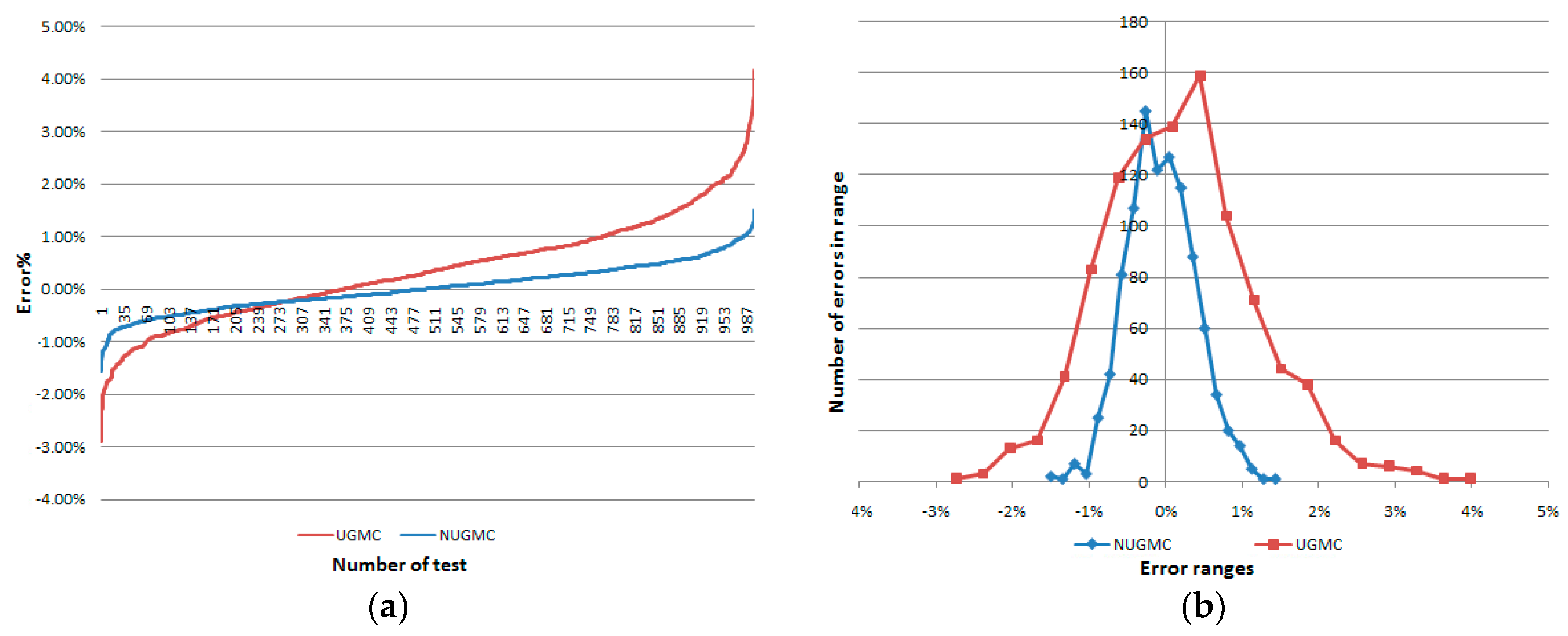
To study the dispersion of the estimated VF values, they are computed 1000 times for the same example (
Figure 4c,
a = 0.5,
c = 0.6,
b = 0.3, CRF = 9,
Φ = 90°,
delX = 0.01, No. of computations = 3.0 ×10
5), the exact analytic result is 0.17028.
The estimated 1000 VF values with UGMC approach are sorted from smallest to biggest. The calculated negative and positive errors in percent (also sorted) are illustrated in
Figure 7a. They vary from −3.4% to +9.34%. Then the interval between the minimum and maximum error is divided in 20 parts and for each part the associated errors are counted. That statistic is used to create the chart presented in
Figure 7b, which is a histogram of the errors.
6.2. Results for NUGP and NUGMC
Table 5 shows results for inclined surfaces with NUGP approach. Again the exact solution obtained from Feingold’s method [
21] and analytical integration results are used here for validation. For this approach
delX cannot be defined for the receiving surface, because the size of the cells vary increasing from the common edge to the opposite edge. Thus, the table has a column
delX for the emitting surface and a column
Na for the receiving surface. The CRF factor is 1, because all cells of the emitting surface participate in the calculations.
The NUGMC approach is used for the same case and the results are placed in
Table 6. It is like
Table 5 (for the same VF), only the value of CRF varies and this has influence on the error, time taken and number of computations. The Monte Carlo approach uses random numbers and thus the results of the computation of VF vary (see row 1 and row 2 in
Table 6, where the error of the computed VF for the same case is different). The error is unpredictable, sometime the increase of CRF leads to reduction of time (which is expected) and to a smaller error (which is unanticipated, e.g., see rows 5–8 of
Table 6).
As in
Section 6.1, two charts are prepared with NUGMC and displayed in
Figure 8. First of them is generated using calculated and sorted 1000 errors for the case in
Figure 4c (
a = 0.5,
c = 0.6,
b = 0.3, Φ = 90°, CRF = 9,
delX = 0.01,
Na = 50), the second image is a histogram of the same errors, which vary from −1.56% to +1.51%. It is clear that the errors display an almost normal distribution (Gaussian curve).
There exists another way to generate approximately the same number of computations of NUGMC with CRF = 9 (6.93 × 10⁵). This is when NUGP is used with cells 3 times bigger than in NUGMC approach, which means that the number of cells is 9 times less. The difference between the two approaches is that with NUGMC the centre of 1 random cell of a cluster of 9 cells is used, and in the case of NUGP the centre of a grid containing 9 cells (3 × 3 cells) is used. The error for the NUGP approach for this example is constantly 0.005% for the same number of computations, while for NUGMC it varies from −1.56% to +1.51%.
6.3. Comparison of All Results for Uniform and Non-Uniform Reflectance
To compare both approaches with implemented Monte Carlo method, two sets of 1000 tests with the same number of computations (7 × 10
5) are illustrated in
Figure 9. They clearly explain why the NUGMC approach is better than UGMC—the curve of NUGMC errors (in blue) in
Figure 9a is closer to 0, and the error histogram of NUGMC (in blue again) is more symmetrical, more narrow and closer to 0%.
Additionally,
Table 7 is prepared to compare the performance of the four approaches presented here. It includes results for all approaches for the same case (in
Figure 4c) with almost the same number of computations. The smallest error (0.005%) belongs to NUGP approach, which is 454 times lower than for UPG (2.274%). The errors for the approaches that use MC method vary, thus they are estimated as MAPE% according Equation (8) for 1000 tests. The MAPE% for NUGMC is 2.3 times lower than for UGMC approach.
Next,
Table 8 is prepared to compare the performance of the four approaches for the case of non-uniform reflecting surface. It includes results for all approaches for the same case (in
Figure 4c) with almost the same number of computations, using Equation (5) instead of Equation (4). The albedo of the horizontal reflecting surface varies from 0.2 to 0.8 (see
Figure 10a). The smallest error (0.006%) belongs again to NUGP approach, which is 422 times lower than for UPG (2.531%). The errors for the approaches with MC method are estimated as MAPE% according Equation (8) for 1000 tests. The MAPE% for NUGMC is 2.1 times lower than for UGMC approach. In general for both approaches with MC, the error is unpredictable and varies in large ranges. The grids for NUGP and NUGMC approaches with corresponding colourised VF are displayed in
Figure 10b,c. Both coloured grids look similar, but they are not the same because of the randomised calculations in NUGMC.
From a practical point of view, if we consider any case of two surfaces exchanging radiant energy, we find that both emitting and receiving surfaces are in majority of cases non-uniform with respect to their radiative properties. In this case, it is difficult to use the classical, calculus-based approach to obtain the view factor. The only procedure left is to use a finite-element based approach in which the surfaces are divided into elements for which the radiative properties may be prescribed individually. That is the chief advantage of all presented techniques. Furthermore, it is important to keep the computational time to a minimum. In this article time-saving, efficient routines are presented that address the above issues.
All four considered approaches could be used for non-uniform emitting and reflecting. These with MC method (UGMC and NUGMC) can be used for a fast evaluation of the energy exchange, when the time saving is desirable. This could allow a fast energy “preview” and comparison of different building designs. It has to be underlined that all these four approaches are not suitable for specular reflecting.
Table 9 include information about the advantages and disadvantages of the four considered approaches, which are compared using the following criteria: ease of programming, computational execution time, accuracy of results obtained, and predictability of the errors.
7. Conclusions
This article presents four approaches for the estimation of view factors as a measure of radiation exchange between surfaces. All of them are based on a micromesh, finite-element approach. Broadly speaking two types of geometries were considered—surfaces that were perpendicular to each other, and those that were at an obtuse angle. Two approaches—UPG (Uniform Populous Grid) and UGMC (Uniform Grid Monte-Carlo) use regular mesh for both emitting and receiving surface; the other two—NUGP (Non Uniform Grid Populous) and NUGMC (Non Uniform Grid Monte Carlo) use non-regular mesh for receiving surface only, the emitting surface is divided into a uniform grid. Two approaches (UGMC and NUGMC) use a hybrid Monte Carlo method to decrease the number of computations, the hybrid method resulting from the present work. Between these two approaches the following conclusions may be drawn: using the Monte-Carlo approach offers a powerful tool to reduce the number of computations without compromising the error. In one case, for example, with the error around the 0.01% mark with the Monte-Carlo approach it is possible to reduce the computations from 436 million to 43.6 million without any significant change in accuracy. The respective computer time taken for the execution of those routines was 674 and 109 s. Another remarkable finding of the present research was that owing to its purely random nature the Monte-Carlo method may reduce a significant amount of computational effort while reducing the error at the same time. To give an example for the case when the two surfaces were at an angle of 135 degree the Monte-Carlo approach reduced the error from 0.407% for uniform grid to 0.124% while using a Computational Reduction Factor of 100. So, it is possible to get a double bonus—reduced computations and higher accuracy.
Finally a comparison of advantages and disadvantages of all four considered routines was added, using the following criteria: ease of programming, computational execution time, accuracy of results obtained, and predictability of the errors.
The order in which the present routines may be arranged with respect to increasing accuracy are UPG followed by UGMC, NUGMC, and NUGP.
Table 7 and
Table 8 numerically sums up these findings for uniform and non-uniform reflectance, i.e., for the same number of computations the NUGP approach is most accurate, it is about 450 times (430 for non-uniform reflectivity) more accurate than UPG, 160 (125) times more than UGMC, and 70 (60) times more than NUGMC. This demonstrates the potential of the NUGP approach. There is scope for further development of this work.


