Novel Time Method of Identification of Fractional Model Parameters of Supercapacitor

Abstract

Accurate dynamic models of supercapacitors (SCs) are a basis for the design, control and exploitation of the hybrid energy storage systems for electric vehicles. This paper concerns a fractional model of SC impedance, based on the Cole–Cole equation describing relaxation in electric double layer. This article provides a new method of identifying the parameters of fractional order model of SC impedance, performed without disconnecting the SC module from the energy storage system. The test drive for this purpose needs only the respect a few simple recommendations. The article presents the conditions of the mentioned test drive that will ensure the frequency spectra of the recorded signals lying in the bandwidth necessary for the correct identification of the model parameters. These parameters are determined by means of the Nelder–Mead simplex optimization method. The results of the identification described by the time method coincide with those obtained in the frequency domain. It has been shown in the last part of the article that the real energy losses in these systems significantly exceed the losses determined only on the basis of the nominal capacity and series equivalent resistance (ESR), to which the SC catalogue data are usually limited. This paper also provides an auxiliary frequency criterion for the selection of SCs intended for energy storage systems of electric vehicles.

1. Introduction

Accurate dynamic models of supercapacitors (SCs) are a basis for the design, control and exploitation of the hybrid energy storage systems (HESS) for electric vehicles [1,2]. The use of these models enables us to efficiently save energy and to control the degree of wear out of SCs used as HESS elements. In such systems, SCs complement the main energy sources (batteries), because compared to them, SCs have higher power density. SC modules are used as a source of additional power in the vehicle acceleration phases. In addition, they absorb braking energy, thus preventing unnecessary energy loss. Due to the high power of the SC modules used in vehicles, the identification of their dynamic model parameters is significantly hindered. This article describes a new method of identifying parameters of fractional SCs models without taking SCs out from the vehicles while respecting the conditions of their normal operation.

The literature presents numerous descriptions of SC impedance models [3,4,5], among others the fractional order models [6]. The fractional models of SC [7,8,9,10,11] can be associated with physical phenomena in the electric double layer [12] and at the same accuracy of dynamics description are less complex than the models of integer order [5,13]. Due to the smaller number of parameters and their relationships with physical phenomena, they are easier to identify.

The identification of parameters of the dynamic models is carried out in laboratory conditions with deterministic signals or in operating conditions with stochastic signals [14]. In the first case, the identification can be based on examining the cells of SC modules by exciting them with pulses or waves of current, and then processing their voltage responses. When testing the parameters of complete SC modules in electric vehicles, identification carried out in similar manner would require the use of high power current generators. Therefore, in this case, it is advisable to use the results of SC voltages and currents recorded during the vehicle ride. However, due to the random nature of these signals, such an identification in the classical approach can be inefficient and often inaccurate. To solve this problem, the authors suggest a new identification method based on the results of a short test ride that meets the specific requirements.

It was assumed that during the test drive, the SC modules have an unchanged configuration within energy storage system. The identification process due to the accelerations cannot be excessively burdensome for the driver and possible passengers. The requirements for the test drive should be simple, but the resultant frequency spectrum of current signals must be sufficient for the full identification of the parameters of the fractional SC model. It was assumed that the values of parameters of a given model will be based on optimization calculations, leading to the similarity of the respective input/output signals of the model with those experimentally recorded.

At the beginning of the paper, there is a brief description of the applied fractional model of SC impedance, based on our own and cited works. Significant frequency sub-bands of the SC impedance characteristics are specified. Then the requirements set by the authors for the process of identifying the parameters of this model in the vehicle operating conditions are presented. These requirements affect the limits of permissible current excitations. In the result of the analysis, the trapezoidal pulse was adopted for the SC model test current. The spectral analysis of this pulse is performed.

The principles, methods and the results of optimization calculations carried out for the SC incited with trapezoidal current pulses for the signals registered during the laboratory tests are presented.

2. Impedance of a Supercapacitor

The SC dynamic model can be presented in the form of the impedance, whose equivalent diagram is shown in Figure 1. The value of capacitance C is related to the properties of the electric double layer. A phenomenon of dielectric relaxation occurs in this layer [12], and therefore the capacity is a function of frequency C(jω). The resistance R_C corresponds to the series equivalent resistance (ESR).

The resistance R_U represents the leakage in the SC model. This leakage is low and has a negligible influence on the storage dynamics, so its typical value can be assumed in the equations. As a result, R_U is not covered by this identification. The presented dependencies can also be simplified because

$$\frac{R_C}{R_U}\cong 0.$$

(1)

Due to the discussed use of SC in the energy storage systems, the description may omit the inductance L, whose significant effect is visible only at very high frequencies. As a result, the frequencies considered in the article do not exceed the band of f_min = 0.1 mHz and f_max = 100 kHz.

The phenomenon of dielectric relaxation in SC is often described by the Cole–Davidson [8,12] or Cole–Cole [11] equations. This article will use the Cole–Cole equation, because it leads directly to the canonical form of fractional impedance [6]. The electrical permeability Cole–Cole equation for electrical double layer has the form [12]

$${\epsilon }_{CC}\left(j\omega \right)={\epsilon }_{\infty }+\frac{{\epsilon }_s-{\epsilon }_{\infty }}{1+{\left(j\omega T\right)}^{\delta }},$$

(2)

where

ω—angular frequency,

ε_∞—permittivity at the high frequency bound,

ε_s—static, low frequency permittivity,

T—the characteristic relaxation time,

δ—coefficient chosen empirically.

If in Figure 1 inductance is omitted, the impedance of the presented system is

$$Z_{cc}\left(j\omega \right)=R_c+\frac{R_u}{1+s{R}_{u}C\left(j\omega \right)}=\frac{\left(1+\frac{R_c}{R_u}\right)+j\omega R_{c}C\left(j\omega \right)}{\frac{1}{R_u}+j\omega C\left(j\omega \right)}.$$

(3)

The capacity is proportional to the permittivity. As a result of transformations based on the Cole–Cole equation, assuming ε_∞ = 0 and (1), the parametric model of SC impedance takes on the form

$$Z_{CC}\left(j\omega \right)=\frac{\left(1+\frac{R_c}{R_u}\right)+{\left(j\omega \right)}^{\delta }\left(1+\frac{R_c}{R_u}\right)T^{\delta }+j\omega R_{c}C}{\frac{1}{R_u}+{\left(j\omega \right)}^{\delta }\frac{T^{\delta }}{R_u}+j\omega C}\cong \frac{1+{\left(j\omega \right)}^{\delta }{T}^{\delta }+j\omega R_{c}C}{\frac{1}{R_u}+{\left(j\omega \right)}^{\delta }\frac{T^{\delta }}{R_u}+j\omega C}.$$

(4)

Due to the adoption of a typical R_U value, the discussed identification of model (4) parameters involves the determination of four parameters: C, R_C, T and δ.

The exemplary results of measurements of the SC frequency response and its compliance with impedances, described by models using the Cole–Cole equation (C-C) and a similar Cole–Davidson equation (C-D), are shown in Figure 2. Three sub-bands can there be distinguished. Arbitrary ±15° phase margins from −90° and 0°, that is −75° and −15°, were chosen as the boundaries between these sub-bands. These sub-bans can be defined as:

(I)

Low frequency band from f = f_min, in which the characteristics are similar to those of an ideal capacitor. The phase is close to −90°, and the module slope is about −20 dB/frequency decade.

(II)

Medium frequency band, in which the impedance phase angle changes from values close to −90° to values close to 0°, and the module has a slope less than −20 dB/decade [15]. This is the sub-band of significant relaxation influence on the frequency response, extending in Figure 2 for about two decades, from f_g1 = 0.003 Hz to f_g2 = 0.4 Hz.

(III)

High frequency band up to f = f_max, in which the characteristics is mainly shaped by the ESR. The phase angle is close to 0°, and the module value does not change much.

The detailed analysis of the relationships (4), as the sum of the three components, related to these sub-bands, can be found in [15].

It should be added that the boundary values of the frequency sub-bands shown in Figure 2 are typical for SC, as they are associated with physical phenomena in the electric double layer.

3. Assumptions for Identification of the Model Parameters

As mentioned earlier, to identify the parameters of the model, one should use the signal, whose spectrum has a significant amplitude in the frequency band, sufficiently describing the dynamics of the model. It follows that the spectral limits of the excitation signal should at least be close to the limits of sub-band II (Figure 2). On the other hand, the presented method also sets the requirements resulting from practical premises.

One of the requirements is that the identification process due to acceleration is not excessively annoying for the driver and possible passengers. The driving torque of the motor is approximately proportional to the motor current supplied, among others, from SC. The elimination of excessive jerks of the vehicle as a result of sudden changes in the driving torque may require limitations of the high frequency components of the current spectrum. This issue is discussed in the article later.

The method of identification of the SC model parameters also depends on the SC module connection with other energy storage blocks realized via bidirectional DC/DC converters based on the switchmode principle, which generates the current and voltage ripples. At high currents and voltages, the 20 kHz switching frequency is most often used, e.g., [16,17]. For this reason, this frequency will be used in the article for comparative purposes

SC current and voltage pulsations and ripples to some extent complicate the identification process. On the other hand, using harmonic analysis, the SC impedance for the converter switching frequency can be determined on their basis. This concerns the R_C parameter of the presented model and ESR impedance, given in the SC catalogs. Manufacturers use several methods to determine ESR values: IEC method [18], “DC 10 ms” [19], individual own methods [20] and the AC method for 1 kHz [21,22]. The graph of a typical ESR changes in the band from 1 kHz to the switching frequency of the DC/DC converter, assumed as 20 kHz, is shown in Figure 3. The graph shows that the changes in ESR are in a practice negligible in this band. This is also confirmed by the results of the authors’ own research, presented in Figure 2.

If the R_C value is determined separately, the number of model parameters necessary to identify decreases from 4 to 3, which significantly simplifies the optimization calculations. In addition, the signals that do not have spectral components in band III, i.e., for high frequencies, can be accepted for identification purposes. It is also a fulfillment of the postulate to eliminate rapid changes in the driving moment of the vehicle.

As mentioned, for the identification purposes, it is necessary to record the current and voltage waveforms of the SC modules during the test drive while meeting the specified requirements. Preparation for identifications needs to stop the vehicle for a period of at least 15 min, necessary for full decay of transients in the energy storage system. Then follows the two-step recording of the SC module current and voltage. The first step consists of accelerating the vehicle from standstill, while the second step is a free run for a few minutes without strict requirements. During the acceleration step, the following conditions were assumed:

• Gradual increase in SC load current, close to a linear increase from zero to the maximum value in about 1 s time, obtained by the appropriate programming of the torque (locomotive) or by a gentle pressing of the accelerator pedal of the bus or car,
• maintaining high constant SC load current for a period of about 10 s, by programming a constant torque or holding the accelerator pedal in constant (maximal) position,
• gradual switching off the SC load current, close to a linear decrease to zero in about 1 s, analogically to acceleration.

The task of step I is to stimulate SC with a high-amplitude current pulse, containing the higher frequencies of the spectrum, desired to identify model parameters. Some deviations from the reference current shape considered below are not very significant due to the registration of the actual excitation. Step II is already a classic identification with random signals. The total duration of both steps must ensure the recording of signal spectrum components in the lower part of the necessary frequency band.

For further analysis of a typical current shape in step I, the trapezoidal pulse was taken on as the reference. The influence of step II was treated as the collection of additional random information. The current during step II can result from the braking or/and acceleration of the vehicle. The analysis presented here concerns the simplest variant, i.e., the zero SC current in the step II.

4. Fourier Transform of a Trapezoidal Pulse

The Fourier transform of a unitary step often used to identify the dynamic parameters has a form

$$ℱ\left[1\left(t\right)\right]=\pi \delta \left(\omega \right)+\frac{1}{j\omega },$$

(5)

The input signal of the capacitor is current, which is integrated. For such systems input current pulses of limited duration are used. For the case when the value of i_P1(t) signal for −T/2 < t < T/2 is 1 and 0 outside this band, the signal’s Fourier transform is

$$ℱ\left[i_{P1}\left(t,T\right)\right]=I_{P1}\left(\omega ,T\right)=T\frac{sin\left(\frac{\omega T}{2}\right)}{\frac{\omega T}{2}}=Tsinc\left(fT\right),$$

(6)

where ω = 2πf. The graph of I_P1(ω,T) modulus for T = 10 is in Figure 4.

The form of denominators of the step (5) and of the pulse (6) transforms decide that their spectra are suppressed in proportion to the increase in frequency. For the square pulse, there is an additional limit sinc(x) ≤ 1. For a general description of the analyzed spectral attenuation, a standardized equation of the envelope can be used, limiting the modulus of the function sinc(fT) from the top and tangent to its local extremes, in the form

$$I_{p0}\left(\omega ,T\right)=\{\begin{array}{cc}1& for f\le f_g\left(T\right)\\ \frac{1}{\pi fT}& for f>f_g\left(T\right)\end{array},$$

(7)

where the break point frequency is

$$f_g\left(T\right)=\frac{1}{\pi T},$$

(8)

This function, with an amplitude adapted to I_P1(ω,10), is shown in the dashed line in Figure 4.

The trapezoidal pulse i_p2(t) can be treated as a convolution of two rectangular pulses in the time domain. With a pulse of width T₁ and amplitude A₁ = 1, and a second pulse of smaller width T₂ and amplitude A₂ = 1/T₂, the result of the convolution is a trapezoidal pulse with an amplitude of 1 (Figure 5). The transform of the convolution is a product of the transforms of both functions. For a trapezoidal pulse i_p2(t) of a unitary amplitude, the Fourier transform is

$$ℱ\left[i_{P1}\left(t,T_1\right)*\frac{1}{T_2}{i}_{P1}\left(t,T_2\right)\right]=I_{P2}\left(\omega ,T_1,T_2\right)=T_{1}sinc\left(f{T}_1\right)sinc\left(f{T}_2\right).$$

(9)

In the case of T₁ = 10 s, T₂ = 1 s, the convolution graph as a function of time is shown in Figure 5. The graph of the transform Ii_p2 modulus is shown on the comparative Figure 4.

The comparison of the trapezoidal pulse I_p2(ω,T₁,T₂) spectrum with the rectangular pulse I_p1(ω,T) spectrum in Figure 4 shows that when T = T₁ >> T₂, the initial part of the graph of the trapezoidal pulse I_p2(f) spectrum modulus differs negligibly from the spectrum modulus of I_p1(f). At higher frequencies, stronger attenuation occurs and additional zero values may emerge for the trapezoidal spectrum.

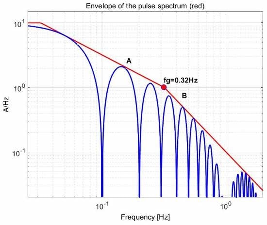
Equation (9) implies by analogy that the envelope of the trapezoidal pulse module is also a product of this type of function for rectangular pulses. For a trapezoid with times T₁ and T₂ and the amplitude of normalized, the equation has the form

$$I_{p02}\left(\omega ,T_1,T_2\right)=I_{p0}\left(\omega ,T_1\right)I_{p0}\left(\omega ,T_1\right),$$

(10)

It is obvious that this function has a second brake point for the frequency

$$f_g\left(T_2\right)=\frac{1}{\pi T_2}=\frac{1}{\pi 1s}=0.32 Hz,$$

(11)

This is illustrated by the double logarithmic graph in Figure 6. In the initial part of this graph, the tangent to the maxima (A) has a slope of −20 dB/decade of frequency, just like for function f_g(T₁). Above the break point f_g(T₂) the tangent (B) has a slope of −40 dB/decade.

The graph also shows that the first minimum of the module, associated with the first element of the transform (9) is for f = 1/T₁ = 0.1 Hz. The influence of the second element of this transform is also clear by lowering the modulus value around the frequency f = 1/T₂ = 1 Hz.

In conclusion, it can be stated that the duration T₂ of the slopes of the trapezoid sets the frequency limit, from which the increased attenuation of the trapezoidal spectrum relative to the rectangle occurs. The value of this limit is determined by the relationship (11).

Discussing the use of the trapezoidal signal spectrum for the identification purposes, one cannot ignore the issue of digital recording of sampled signals in finite time Tc. The discrete frequency spectrum can be obtained as a result of the Fast Fourier Transformation (FFT). The length of time of the signal recording determines the first fundamental frequency of this spectrum. It is

$$f_{\min }=f_1=\frac{1}{T_c},$$

(12)

The envelope of harmonic amplitudes for the trapezoidal pulse is determined by the function

$$E{n}_{P2}\left(\omega ,T_1,T_2\right)=2f_{\min }{I}_{P2}\left(\omega ,T_1,T_2\right),$$

(13)

For a single pulse in Figure 5 with a recording time T_c = 100 s, the graph of the harmonic amplitudes of the in the spectrum and their envelope (13) for lower frequencies is shown in Figure 7. The frequency of the first harmonic in this spectrum is f_h1 = 1/100 s = 0.01 Hz. The sampling frequency used in this case was 100 Hz. As a result, the maximum useful spectrum component, according to Shannon’s law, is limited by a frequency of 50 Hz. It should be added that the frequencies presented in Figure 7 were selected mainly to obtain the readability of the graph. The frequency band necessary for the proposed SC dynamics identification method begins slightly lower.

The single step signal commonly used for identification purposes has a spectral amplitude (5) that decreases with frequency. This kind of spectrum is not an obstacle, e.g., in the analysis of dynamics of the systems, due to the use of logarithmic frequency scales for this purpose, e.g., in Bode plots. For example, Figure 2 presents a graph of the frequency points of the SC impedance characteristics measured for the purpose of identifying the model parameters. The measuring point values represent their surroundings with an increasingly-wider frequency band. In the case of a discrete spectrum in these surroundings, the number of spectral components rises proportionally, compensating for the decrease in their amplitudes. As a result, the limitation of the effectiveness of trapezoidal pulses is their rise and fall time, i.e., the upper frequency limit f_g(T₂), described by the relationship (11) and marked in Figure 6. Above this frequency, the spectrum amplitude decrease occurs with the square of frequency.

It was assumed for the identification process that after excitation with a strong current pulse of possible shortest slopes, a step of free ride follows without strict requirements. For the presentation of the spectral effects of such a ride, let us assume a modification of the previously used single trapezoidal pulse by adding any pulse in the second step of the registration. Figure 8 shows the basic pulse i_trap(t) and the modified i_mod(t). Figure 9 shows the spectrum envelopes for both cases. The modification causes some changes in the envelope at low frequency without significantly affecting the rest. This does not impair the identification process by the method described, because the change in the spectrum is only local, while the modulus and phase of the SC model change monotonically as a function of frequency. The measurement of the real SC current signal allows for some deviations also from the trapezoidal current pulse used in step I. For such modifications of the current signal, the identified model parameters remain practically unchanged.

In the identification process, due to measurement noise and distortions, it is advisable to use a sampling frequency much higher than the mentioned trapezoidal pulse spectrum limit. The use of oversampling and then decimation through a low-pass filter gives a data stream with a modified sampling frequency which is sufficient to satisfy the Shannon’s law. The advantage is that this reduces the level of measurement noise and distortions. To reduce the effect of interference due to the pulse width modulation in the DC/DC converter, the use of an analog anti-aliasing filter before the analog-to-digital converter should be considered. The last remark does not apply, of course, to determining the RC value.

5. Identification Results According to the Proposed Method

To illustrate the application of the described method, one can compare the results of SC identification for a capacitor of 0.47 F by the frequency method, described more widely by the authors in [11] with the results of the method proposed here in this article. The measured points of the frequency response of this SC are shown in Figure 10 with asterisks. On their basis, the impedance model parameters were determined by approximation (4).

The SC model parameters identification, carried out by the authors, was based on the simplex method, which is used in the Matlab fminsearch function. The frequency method uses the following performance index [11].

$$J_f=\frac{1}{N-1}{{\displaystyle \sum }}_{i=1}^N{\left(\frac{\left|Z_{CC}\left(j{\omega }_i\right)-Z_p\left(j{\omega }_i\right)\right|}{\left|Z_p\left(j{\omega }_i\right)\right|}\right)}^2,$$

(14)

where

Z_CC(jω)—impedance approximating the genuine impedance of SC,

Z_P(jω)—measured impedance of SC,

ω_i—angular frequency of ith measurement point.

As the mean value of the relative approximation error it was assumed

$${\sigma }_f=\sqrt{J_f},$$

(15)

The parameter values determination consists of a multimodal minimization of the performance index. That is why it is important to assume appropriate starting values. The relationship between model (4) parameters and physical ones, including the SC catalog parameters, makes this task much easier. Nominal values of capacity C and resistance R_C = ESR can be used as the starting parameters of the model. In the case of identifying the degree of SC wear, these may also be the results of previous identification. A typical value of δ = 0.7 can be taken as the starting value of the exponent δ. The starting value for the relaxation time constant T is of the order of 10 s [24].

Physical limitations of parameter values can pose problems during identification. To solve them, the authors used a very large nonlinear increase in the performance index for negative values of optimized parameters and for the exponent δ exceeding the value of 1. In the case under consideration, deterministic optimization is sufficient to obtain unequivocal results, although some authors solve similar tasks by probabilistic methods, e.g., GWO [25].

As a result of the calculations, the following impedance model of 0.47 F SC was obtained

$$Z_{ccf}\left(\omega \right)=\frac{1+12.7s^{0.594}+15.5s}{5.07E-07+6.37E-06s^{0.602}+0.572s},$$

(16)

In Figure 10, the impedance characteristic (16) is marked with a red dotted line.

Later in the study, the SC was excited by a trapezoidal current pulse. This pulse, along with the initial phase of the SC voltage response, is shown in Figure 11. The response recorded within 250 s became the basis for determining the parameters of the model (4) using the time method. The full analyzed SC voltage response is shown in Figure 12 in the form of solid line.

The method described in this article is based on minimization of the mean square error of the model response related to the actual response with the same excitations. The assumed performance index was

$$J_t=\frac{1}{N-1}{{\displaystyle \sum }}_{i=1}^N{\left(u_{CCi}-u_{pi}\right)}^2,$$

(17)

where

u_Pi—ith sample of SC voltage,

u_CCi—ith sample of the SC model response to the same excitation,

$N$—the number of time response samples.

The standard deviation of the relative approximation error of the model response is

$${\sigma }_t=\sqrt{\frac{{{\displaystyle \sum }}_{i=1}^N{\left(u_{CCi}-u_{pi}\right)}^2}{{{\displaystyle \sum }}_{i=1}^N{\left(u_{Pi}-\overline{u_P}\right)}^2}}=\sqrt{\frac{J_t\left(N-1\right)}{{{\displaystyle \sum }}_{i=1}^N{\left(u_{Pi}-\overline{u_P}\right)}^2}},$$

(18)

where $\overline{u_P}$ is the mean value of SC voltage.

The fractional impedance determined in this way, based on the Cole–Cole equation, has the form

$$Z_{cct}\left(\omega \right)=\frac{1+20.5s^{0.707}+15.1s}{5.0E-07+1.03E-05s^{0.707}+0.560s},$$

(19)

The frequency response diagram of this impedance is marked with the letter “b” in Figure 1.

Comparing the frequency characteristics measured and those of both considered models, presented in Figure 10, it can be concluded that the differences between them are small. We can also compare the coefficients of models (16) and (19). The values partly related to physical parameters are presented in

Table 1. The comparison of SC models.

Nominal Capacitance	Identification Method	Model Parameters				Error		WII
		Capacitance	ESR	δ	Tδ	ϭf	ϭt
0.47 F	frequency	0.57 F	27 Ω	0.59	13	5.0%	23%	750
	time	0.56 F	27 Ω *	0.71	21	20%	6.3%
10 F	frequency	14.5 F	101 mΩ	0.18	0.69	4.9%	4.1%	24
	time	14.6 F	101 mΩ *	0.17	0.59	5.8%	2.9%

* adopted on the basis of frequency measurement.

. Due to the experimental selection of the coefficients δ and T^δ, there is no explicit physical interpretation.

Similar tests were also made for other types of SC. The results are presented in Table 1 and in Figure 13 and Figure 14. Both cases presented in Table 1 are characterized by a very different relative width of the II frequency sub-band, equal to

$$W_{II}=\frac{f_{g2}}{f_{g1}},$$

(20)

In the case of film capacitors for the model of Figure 1, it can be assumed that C(jω) and ESR are constant. Then the considered coefficient is smaller and amounts to W_II = 14.

The differences in the W_II value can also be noticed in the shape of the time response to pulse excitation and in the energy efficiency of the SC. These issues are presented in this article later.

The results presented in Table 1 and in Figure 10, Figure 12 and Figure 13 show that the frequency and time methods presented here lead to similar results. Slightly larger differences occur for very large W_II values. However, the next part of the article shows that these cases are irrelevant for the SCs working in HESS.

6. Energy Losses in SC Module of HESS

Energy losses in SC depend on ESR and dielectric relaxation, described by the Cole–Cole Equation (2). The analyzed SC impedance model (4) allows us, among other things, to calculate the efficiency of the SC module for various operating conditions. The test for the SC charge and discharge cycle corresponding to the vehicle cycle, consisting of braking, short stoppage and acceleration of the vehicle will be presented below. The following assumptions were made for the research:

• Due to the requirement of the minimum value of supplied power at a given current, the instantaneous voltage SC u_SC(t) does not fall below half of the permissible SC operating voltage U_max/2. This voltage also does not exceed the maximum value of U_max. The current pulse amplitude has a possible maximum value for these conditions.
• Supply and consumption of the energy is carried out by single i_SC(t) pulses of the shape as in Figure 5. Both pulses have identical amplitudes, therefore the SC electric charge at the end of the cycle is equal to the initial charge. The interval between pulses is 10 s, which corresponds to a short stop of the vehicle.
• The initial voltage SC u_SC(0) is 75% of the permissible voltage U_max and this is in a steady state. The choice of such a value ensures that the voltage is maintained within the assumed limits regardless of the polarization of the initial current pulse.

For the tested SC units with a capacity of 0.47 and 10 F, the voltage and current waveforms are presented in Figure 15 and Figure 16, respectively. The energy supplied by the first pulse is

$$E_{+}=\begin{array}{cc}{\displaystyle \int }{i}_{SC}\left(t\right)u_{SC}\left(t\right)dt& for i_{SC}\left(t\right)>0\end{array},$$

(21)

and the energy received by the second pulse has a value

$$E_{-}=\begin{array}{cc}{\displaystyle \int }{i}_{SC}\left(t\right)u_{SC}\left(t\right)dt& for i_{SC}\left(t\right)<0\end{array},$$

(22)

and the energy received by the second pulse has a value

$${\eta }_{SC}=\left|\frac{E_{-}}{E_{+}}\right|,$$

(23)

The results of efficiency measurement in the above test are presented in

Table 2. Energy efficiency of SC for test conditions.

Capacitance SC	0.47 F	0.1 F	10 F
Frequency response	Figure 10	Figure 2	Figure 13
Coefficient WII	890	120	27
Real efficiency	65%	73%	91%
Efficiency for C(jω) = const (ESR losses only)	87%	88%	94%
ESR losses/total losses	37%	44%	67%

for three SCs. They differ in the width of sub-band II. SCs of capacitance 0.47 and 10 F have W_II coefficients near-extreme cases. In the table, the actual efficiency values are compared with the results obtained for the same excitation for the simplified model with C(jω) = const and the ESR determined for the III frequency sub-band in accordance with the catalog data. In Table 2, the energy losses include only Joule–Lenz losses in ESR, which are only a part of the total losses.

The comparison of the SC voltage response simulation of the fractional order model and the simplified model mentioned above is shown in Figure 16. The difference of the two increases with the coefficient W_II.

The comparison of values in Table 2 confirms the legitimacy of using the described fractional SC impedance model for a reliable loss calculations, because the data normally provided in the SC catalogs are usually insufficient for such purposes. The possibility to determine the actual SC voltage waveforms also allows for the optimization of the electric vehicle energy storage control. These issues are discussed more extensively e.g., in [1,2,6].

7. Conclusions

Extensive use of HESS in electric vehicles requires testing their SC modules in operating conditions. This article provides a new method of identifying the parameters of fractional order model of SC impedance, carried out without disconnecting the SC module from the energy storage system. It is based on the results of SC voltage and current recording during a short, easy to implement test ride. The conditions of this test are given. They are based on the spectral analysis of the SC current pulses occurring during this test.

By means of the simplex method optimization calculations based on the recorded voltages and currents are applied. As a result, the values of the parameters of the fractional SC impedance model are determined. This article gives the method of performing these calculations and their sample results. An example of the use of this model is the analysis of the energy efficiency of an SC that is a part of the HESS.

The presented fractional SC model with correctly identified parameters reproduces dynamic properties of its physical counterpart with high accuracy. Therefore, it can also be used to design hybrid energy storage systems for electric vehicles and their control systems. Checking the parameters changes of these models can make it possible to estimate the wear out of components.

An additional conclusion is that when selecting SC types for operation in HESS, it is reasonable to follow the low value of the W_II coefficient of the bandwidth II of the SC frequency characteristics. This can be a supporting frequency criterion for the selection of SCs intended for energy storage systems of electric vehicles