A Sparse Spike Deconvolution Algorithm Based on a Recurrent Neural Network and the Iterative Shrinkage-Thresholding Algorithm

Abstract

Conventional sparse spike deconvolution algorithms that are based on the iterative shrinkage-thresholding algorithm (ISTA) are widely used. The aim of this type of algorithm is to obtain accurate seismic wavelets. When this is not fulfilled, the processing stops being optimum. Using a recurrent neural network (RNN) as deep learning method and applying backpropagation to ISTA, we have developed an RNN-like ISTA as an alternative sparse spike deconvolution algorithm. The algorithm is tested with both synthetic and real seismic data. The algorithm first builds a training dataset from existing well-logs seismic data and then extracts wavelets from those seismic data for further processing. Based on the extracted wavelets, the new method uses ISTA to calculate the reflection coefficients. Next, inspired by the backpropagation through time (BPTT) algorithm, backward error correction is performed on the wavelets while using the errors between the calculated reflection coefficients and the reflection coefficients corresponding to the training dataset. Finally, after performing backward correction over multiple iterations, a set of acceptable seismic wavelets is obtained, which is then used to deduce the sequence of reflection coefficients of the real data. The new algorithm improves the accuracy of the deconvolution results by reducing the effect of wrong seismic wavelets that are given by conventional ISTA. In this study, we account for the mechanism and the derivation of the proposed algorithm, and verify its effectiveness through experimentation using theoretical and real data.

1. Introduction

Sparse spike deconvolution is a common high-resolution processing method that aimed to seismic data. In this method, reflection coefficients are first estimated from a band-limited seismogram, and then a high-resolution seismogram is obtained based on the previously determined reflection coefficients. There are a variety of sparse spike inversion algorithms, such as the greedy iterative algorithm based on matching pursuit for sparse signal recovery [1,2] and the convex optimization algorithm based on basis pursuit [3]. Algorithms that are based on basis pursuit have simple structures, which are easy to perform with high computational efficiency, are the mainstream solution methods at present. These algorithms require knowledge of the seismic wavelet in advance. However, this type of algorithm cannot accurately extract seismic wavelets from real seismic data, which restricts its application as sparse spike deconvolution method.

In response to this problem, many studies have been carried out to date and two solutions have been proposed. The first solution applies an overcomplete dictionary method [4] that extends the wavelet dictionary to another one that contains components of multiple frequencies. The computational efficiency of this method is proportional to the size of the wavelet dictionary, because the more complete dictionaries tend to be larger. However, the accuracy of the results depends on the completeness of the dictionary. Accordingly, if the wavelet dictionary is not complete, the results are not ideal. This means that the overcomplete dictionary method relies on a compromise between computational efficiency and accuracy or effectiveness, so that it essentially does not solve the problem. The second solution uses the online dictionary learning method for sparse coding [5]. This method learns how to modify seismic wavelets. Instead of directly using error backpropagation, this method uses error to alternate between modification of the reflection coefficient and modification of the seismic wavelet. However, the calculation error is large with this method.

In this study, we propose a sparse spike deconvolution algorithm based on a recurrent neural network (RNN), like the iterative shrinkage-thresholding algorithm (ISTA). This algorithm uses error backpropagation through time (BPTT) along with RNN to improve seismic wavelets and to solve the issue of inaccurate wavelets. Next, we briefly explain the details of the method and then verify the reliability of the algorithm through experimentation.

2. ISTA Algorithm

It can be seen from the above that the target function of sparse spike deconvolution can be expressed as:

$$\underset{x}{\arg \min }({\Vert y-Wx\Vert }_2^2+\lambda {\Vert x\Vert }_1)$$

(1)

where y is the seismogram, W is the seismic wavelet, x is the reflection coefficient, and $\lambda$ is the regularization parameter, ${\Vert .\Vert }_2^2$ represents the square of Euclid Norm, ${\Vert x\Vert }_1$ stands for the sum of the absolute values of the components of $x$. The iterative shrinkage-thresholding algorithm (ISTA), which is used to solve composite functions of Equation (1), was proposed by Beck and Teboulle [6]. According to the theory of ISTA, when ${\Vert y-Wx\Vert }_2^2$ satisfies the lipschitz continuous, we use the proximal gradient method to approximate Equation (1), so that Equation (1) can be expressed as:

$$\left\{\begin{array}{c}\underset{x}{\arg \min }({\Vert x-p_k\Vert }_2^2+\lambda {\Vert x\Vert }_1)\\ p_k=x_k-\frac{2}{L}{W}^T(W{x}_k-y)\end{array}\right\}$$

(2)

Solving Equation (2) while using the iterative threshold method of linear programming, we have:

$$x_{k+1}=h_{\theta }(x_k-\frac{1}{L}{W}^T(W{x}_k-y))$$

(3)

where $h_{\theta }$ is the soft threshold function, θ is the threshold, L is the Lipchitz constant, and $x_{k+1}$ and $x_k$ are the best reflection coefficients for the $k+1$th and $k$th iterations, respectively. We set $W_e=\frac{1}{L}{W}^T$ and $S=I-\frac{1}{L}{W}^{T}W$ in order to compare with the RNN neural network. Subsequently, Equation (3) can be rewritten, as follows:

$$x_k=h_{\theta }(W_{e}y+S{x}_{k-1})$$

(4)

According to the Equation (4) and Figure 1, the ISTA algorithm has the following three points to be noted: (1) we need to determine the Lipschitz constant. In this paper, we use the maximum value of the eigenvalues of the matrix $W^{T}W$ as the value of L; (2) it is necessary to determine the threshold $\theta$ in the soft threshold function, in this paper the threshold is $\theta =\frac{\lambda }{L}$; and, (3) in the ISTA algorithm, each iteration involves parameter $W_e$; therefore, the results of ISTA are affected by $W_e$, by the above, $W_e$ is related to the seismic wavelet, thus the results of ISTA algorithm are directly limited by the accuracy of the seismic wavelets. However, in practice, it is difficult to accurately determine the seismic wavelets, which restricts the use of traditional ISTA algorithm in deconvolution.

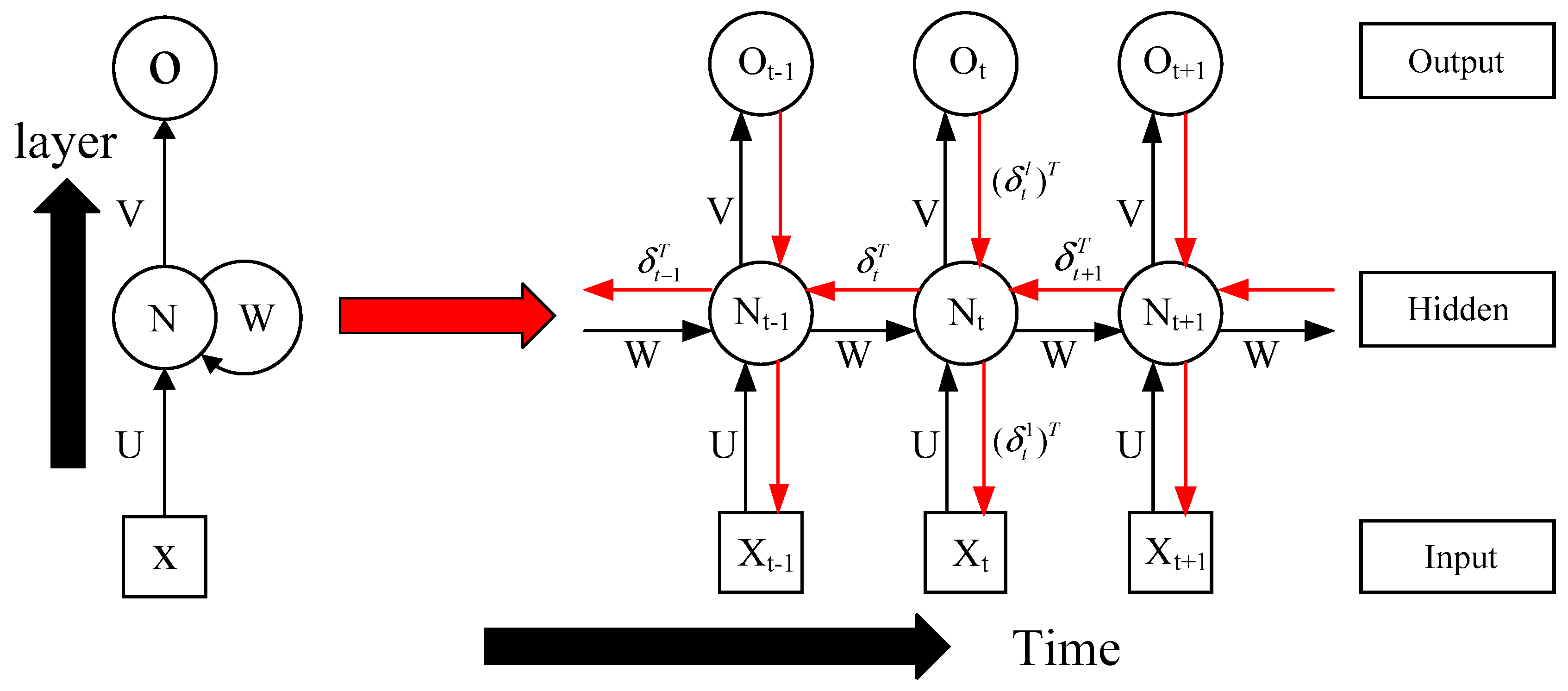
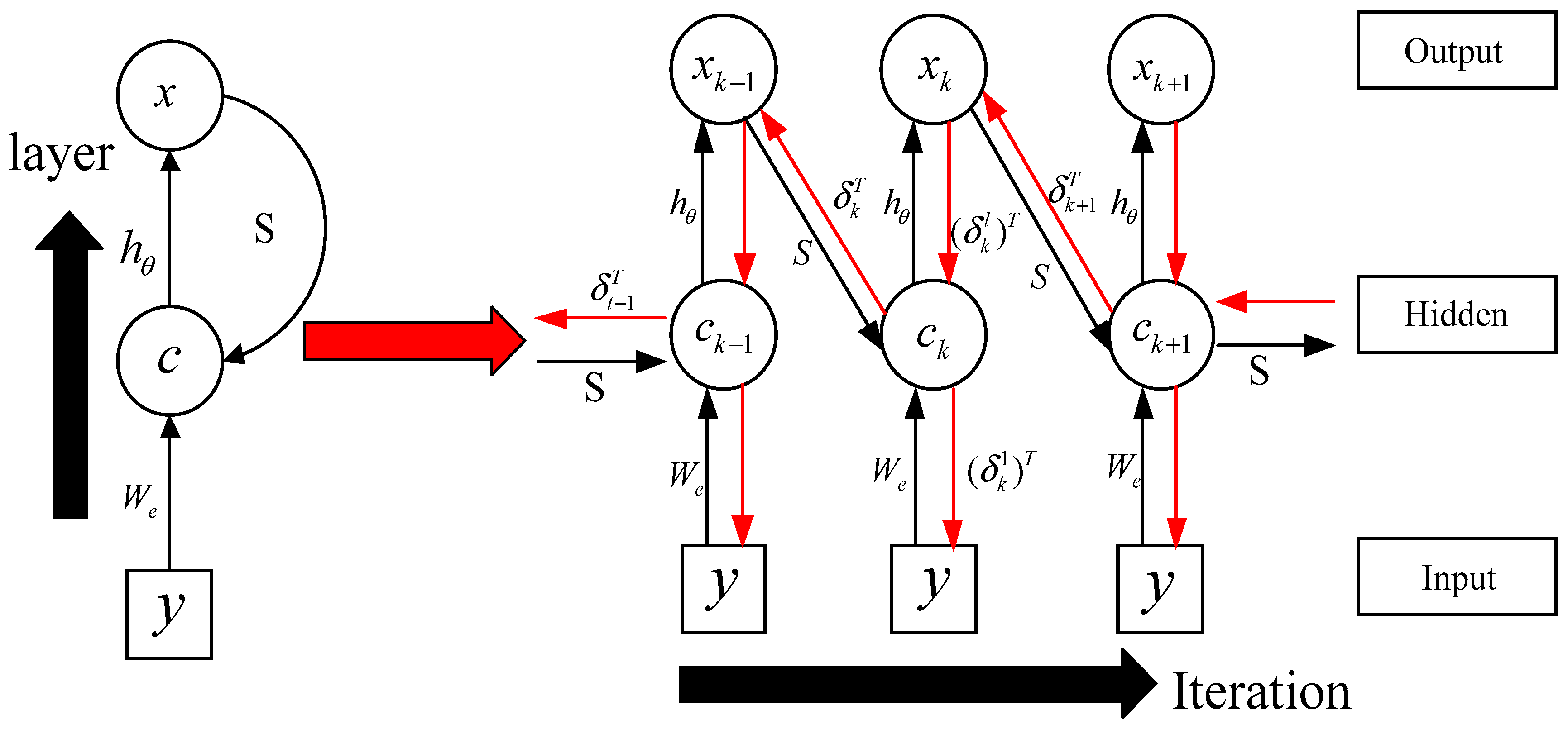
3. RNN-Like ISTA Algorithm

Inaccurate seismic wavelet will affect the solution of ISTA algorithm, according to the discussion above. In order to solve this question, in this section, we propose an RNN-like ISTA algorithm that combine the back propagation in RNN and ISTA algorithm.

RNN is a kind of neural network used to process time series data. In the BP neural network, neural network includes input layer, hidden layer, and output layer. Each layer is connected by the weight function, and the activation function controls the output of the neural network. Traditional neural networks only establish weight function between layers, while the biggest difference between RNN and traditional neural networks is that weight connections are also established in each neurons. [7,8,9].

Figure 2 is the schematic diagram of RNN. In Figure 2, the parameter U represents the weight of the error correction function along the layer, W represents the weight of the error correction function along the time, and parameter V represents the activation function. On the one hand, from the looping style arrow next to the left N in Figure 2, it can be seen that the looping of RNN is reflected in the hidden layer, on the other hand, from the structure expanded on the right, in the RNN, not only are layers connected by weights, but hidden layers of each neuron are also connected by weights; thus, hidden layers of different neurons are interrelated. The RNN includes two main steps: forward calculation and error backpropagation. The RNN-like ISTA algorithm proposed in this paper also includes two steps: forward calculation and error backpropagation.

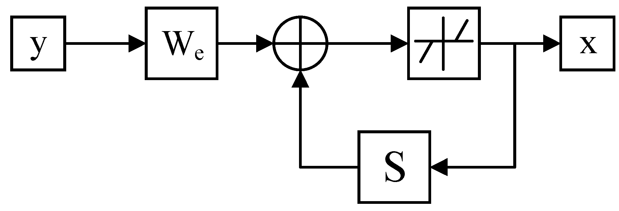
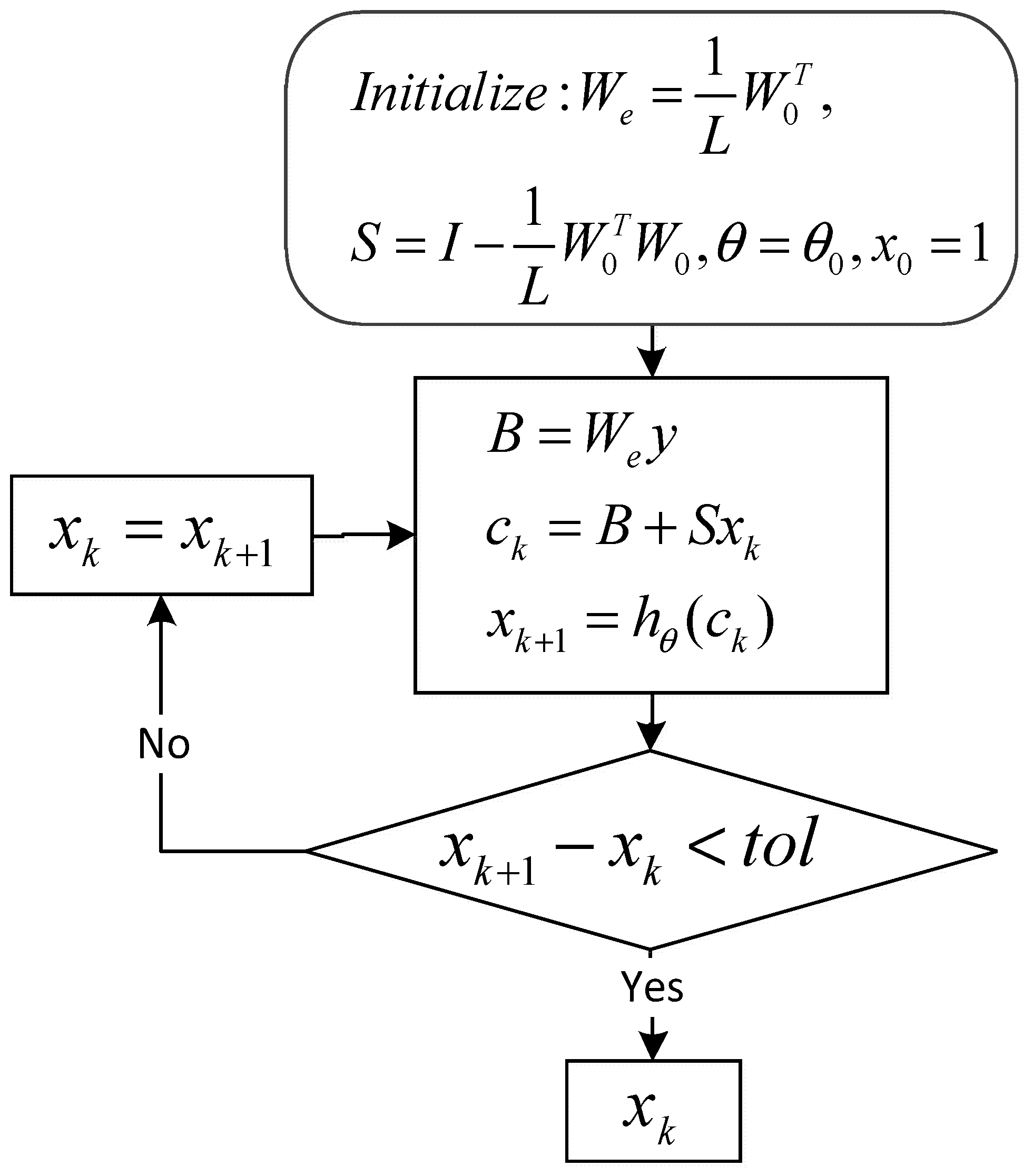
3.1. Forward Calculation

The forward calculation of RNN can be expressed, as above (Figure 2):

$$O_{t-1}=V(U{x}_{t-1}+W{N}_{t-1})$$

(5)

By comparing Equation (4) with Equation (5), we know that the parameter y in Equation (4) is equivalent to the input $x_{t-1}$ in Equation (5), parameter $S$ is equivalent to weights $W$ in the hidden layer, $x_{k-1}$ is equivalent to the hidden layer parameter $N_{t-1}$, and $h_{\theta }$ is equivalent to the activation function V. Accordingly, we can make each iteration in an ISTA algorithm as a time layer in RNN, and make each input variable in ISTA algorithm as a neuron, and make the soft threshold function as the activation function. Therefore, the iterative process of ISTA algorithm can be regarded as the RNN. According to Figure 2, we can obtain the iterative calculation process of ISTA algorithm, as shown in Figure 3, in the iterative calculation process of the ISTA algorithm, since the matrix S participates in each iteration, so its role is similar to the recurrent parameter in the RNN. According to Figure 3, we can get the forward calculation flow chart of RNN-like ISTA algorithm, as shown in Figure 4.

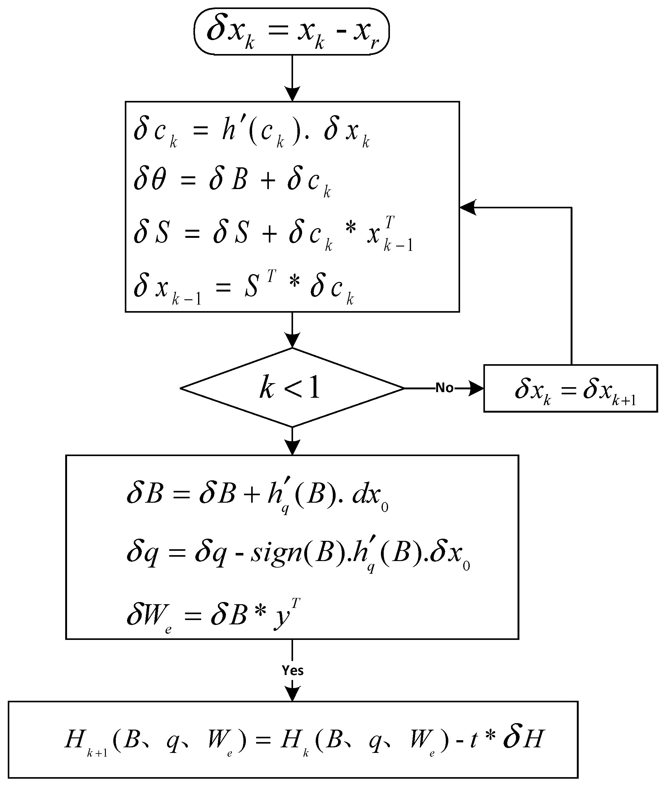
3.2. Error Backpropagation

In this paper, we use the idea of RNN error backpropagation and modify the seismic wavelet through the method of error backpropagation; finally, we can get the seismic wavelet with the characteristics of seismic data. The error backpropagation of RNN usually use BPTT algorithm and the process of BPTT includes three steps: (1) forward calculation of the output value of each neuron; (2) combined with the expected output, calculate the error value of each neuron, and feed the error along the direction of each neuron layer and the time direction of each neuron to each parameter in the calculation process; and, (3) combined with errors, the method of gradient descent is used to modify parameters [10,11].

The red arrow in Figure 2 is the error feedback process, as can be seen from Figure 2, in the process of error feedback, we need to solve to get the error parameters ${\delta }_t^l$. We can obtain the equation of RNN error feedback along the direction of the layer, according to the BPTT algorithm. By using this equation, we can get the error parameter ${\delta }_k^T$ of any layer of the neuron at the certain time:

$${\delta }_k^T={\delta }_t^T{\displaystyle \prod _{i=k}^{t-1}W\cdot diag[\nabla f(ne{t}_i)]}$$

(6)

where diag represents the diagonal matrix, $ne{t}_i$ represents the neuron weighted input at time t, and $\nabla f(ne{t}_i)$ is partial derivative of $ne{t}_i$. In the same way, we can get the equation of error feedback along the formula for the backwards propagation of the error along the time [12]:

$${({\delta }_t^{l-1})}^T={({\delta }_t^l)}^T\cdot U\cdot diag[\nabla f(ne{t}_t^{l-1})]$$

(7)

where ${net}_t^{l-1}$ represents the neuron weighted input in layer l-1 at time t.

We can obtain the error vale at any time of any layer in RNN neural network, and then we need to solve the gradient of weight parameters U and W, in order to update the two parameters by gradient method, according to Equations (6) and (7). For the time direction, we just need to know the error ${\delta }_t$ at any time, and the output value $N^{t-1}$ at time t-1, and we can then find the gradient of the weight matrix at time t. Let the gradient of the parameter W be ${\nabla }_{w_t}E$:

$${\nabla }_{W_t}E=\left[\begin{array}{cccc}{\delta }_1^t{N}_1^{t-1}& {\delta }_1^t{N}_2^{t-1}& \dots \dots & {\delta }_1^t{N}_n^{t-1}\\ {\delta }_2^t{N}_1^{t-1}& {\delta }_2^t{N}_2^{t-1}& \dots \dots & {\delta }_1^t{N}_n^{t-1}\\ \dots & \dots & \dots \dots & \dots \\ {\delta }_n^t{N}_1^{t-1}& {\delta }_n^t{N}_2^{t-1}& \dots \dots & {\delta }_n^t{N}_n^{t-1}\end{array}\right]$$

(8)

where $N_i^{t-1}$ is the output value of the ith neuron in the loop layer at time $t-1$. The gradient of the parameter W is the sum of the gradients at each time [12]:

$${\nabla }_{W}E={\displaystyle \sum _{i=1}^t{\nabla }_{W_i}E}$$

(9)

Similarly, we have the updated gradient of the parameter $U$:

$${\nabla }_{U_i}E=\left[\begin{array}{cccc}{\delta }_1^t{x}_1^t& {\delta }_1^t{x}_2^t& \dots \dots & {\delta }_1^t{x}_m^t\\ {\delta }_2^t{x}_1^t& {\delta }_2^t{x}_2^t& \dots \dots & {\delta }_2^t{x}_m^t\\ \dots & \dots & \dots \dots & \dots \\ {\delta }_n^t{x}_1^t& {\delta }_n^t{x}_2^t& \dots \dots & {\delta }_n^t{x}_m^t\end{array}\right]$$

(10)

$${\nabla }_{U}E={\displaystyle \sum _{i=1}^t{\nabla }_{U_i}E}$$

(11)

Finally, parameter W and U can be updated using Equations (8)–(11) combined with the gradient descent method.

Regarding the BPTT algorithm and considering equation (6) and the operating scheme of RNN-like ISTA (Figure 3), the flowchart of the backward error correction of the improved ISTA is shown in Figure 5.

Where $x_r$ is the expected output, $\delta$ is the error, $B=W_{e}y,c_k=B+S{x}_k$, and sign is the symbolic function. It must be taken into account that the errors in various layers must be first solved step-by-step through a certain number of iterations. Subsequently, the sum of them is calculated to obtain initial input errors $\delta B、\delta \theta$, and $\delta W_e$. Lastly, these three parameters, which are associated with seismic wavelets, are updated using the descent gradient. By combining the forward and backward algorithms, the parameters associated with seismic wavelets can be corrected in successive iterations based on the training dataset. In this way, the most suitable parameters for seismic data can be obtained, which is beneficial for the calculation of deconvolution later on.

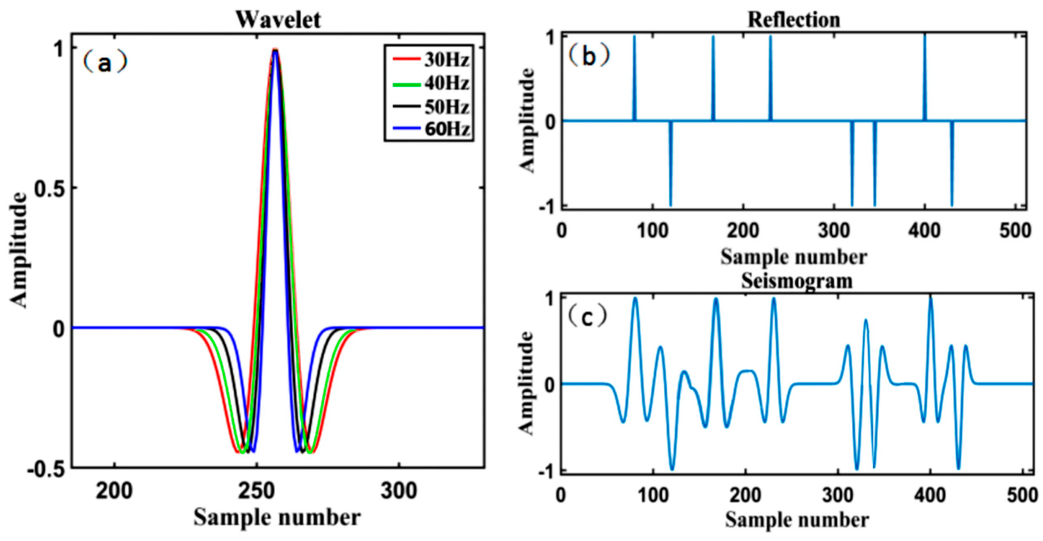
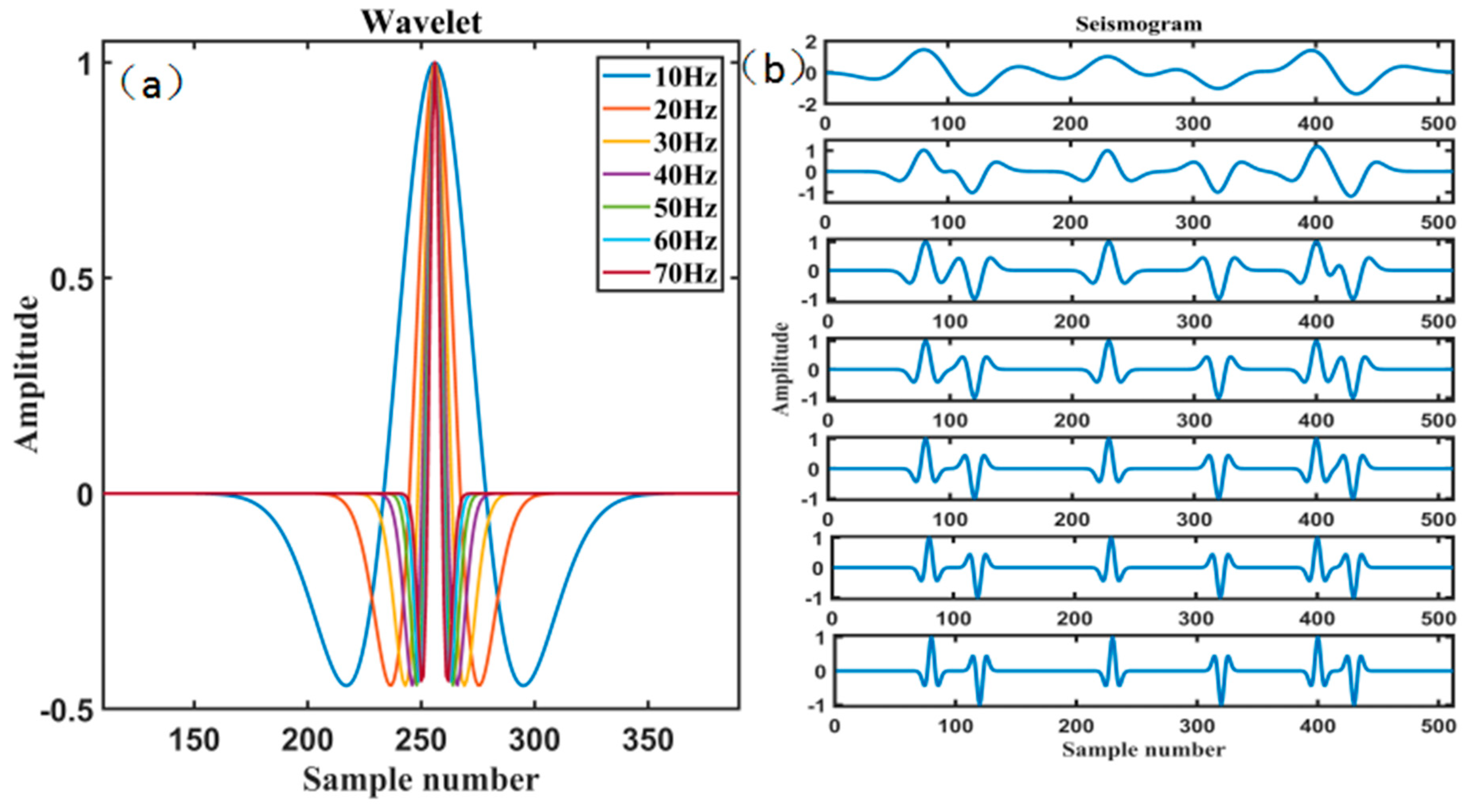
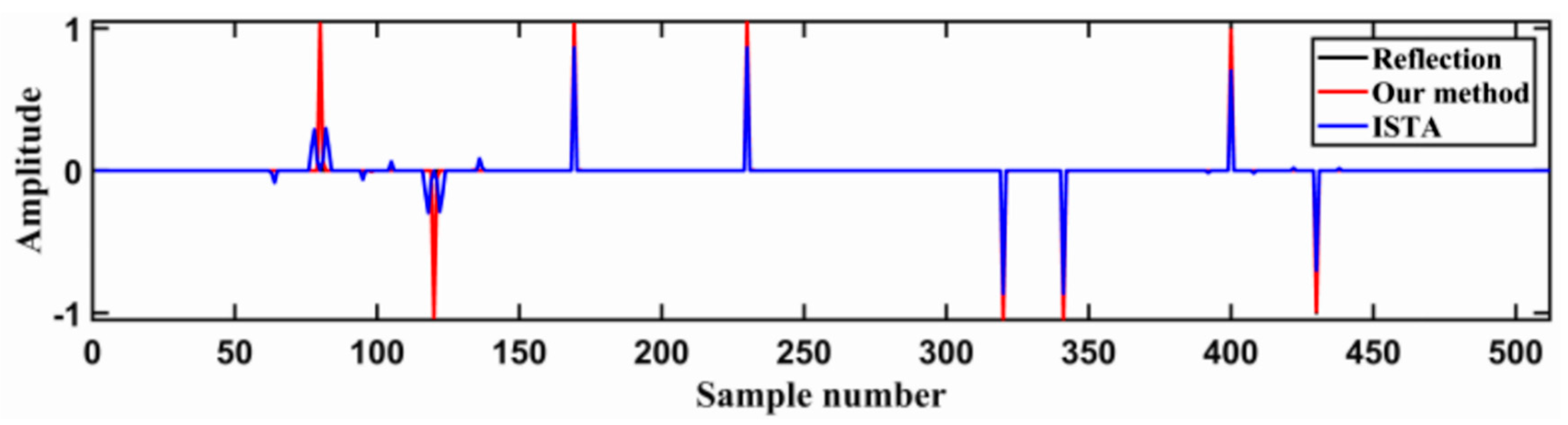
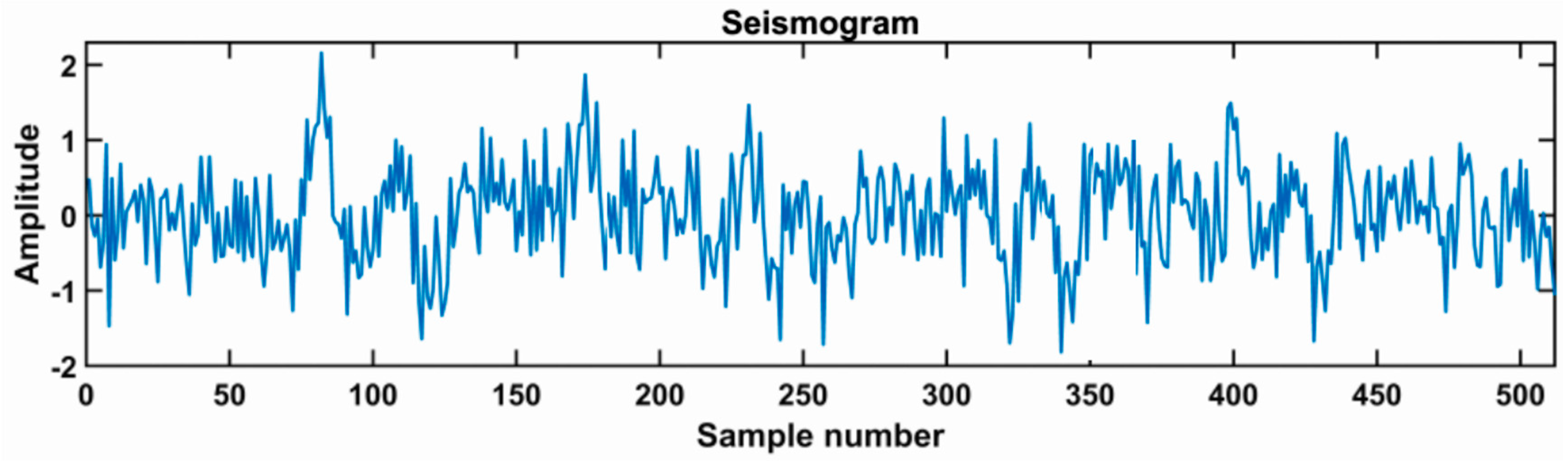
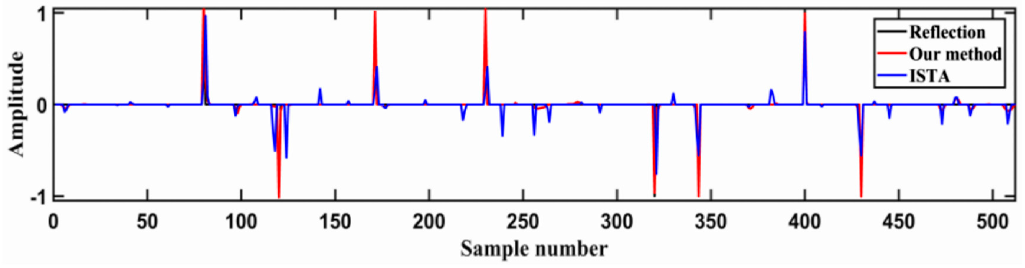
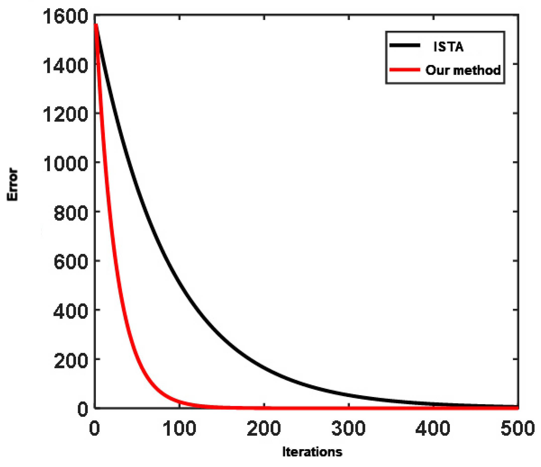
4. Theoretical Model Experiment

In order to verify the effectiveness of the proposed algorithm, theoretical model experiments are carried out in this Section. Firstly, we synthesized a noise-free single seismic record (Figure 6c), which was constructed by convolution of zero-phase Ricker wavelet with frequency of 30 Hz, 40 Hz, 50 Hz, and 60 Hz (Figure 6a) and reflection coefficient (Figure 6b). The trial channel contains 512 sampling points and eight reflection spikes.

The RNN-like ISTA was used to deconvolution the data in Figure 6c below. Firstly, we need to generate training data, we randomly generate a series of reflection coefficients, and then convolute the reflection coefficients with different frequencies of seismic wavelets (Figure 7a), and finally obtain a series of synthetic seismograms (Figure 7b).

The initial input wavelet matrix was set as zero-phase Ricker wavelets at 40 Hz using these data. Combining the forward and backward algorithms mentioned above, the data deconvolution was then performed while using the training seismic wavelets. Figure 8 shows the comparison of this result with that obtained by deconvolution via conventional ISTA using 40 Hz Ricker wavelets. As can be seen, the result of the deconvolution performed with the method proposed in this study is much better than the result provided by conventional ISTA. The position and amplitude of reflection coefficient obtained by RNN algorithm are more in line with the expectation. For example, near the 100th sample point, the number of ISTA algorithm inversion results is far more than the actual number of reflection coefficients. This will cause many errors in the actual inversion work. This demonstrates that the improved method reduces the inaccuracy of the deconvolution results that are usually obtained due to inaccurate initial inputs.

In order to test the noise tolerance of the proposed algorithm, we added random noise to the seismogram shown in Figure 6c in order to have a theoretical model with low signal-to-noise ratio (SNR), such as the synthetic seismogram (SNR = −4.55 dB) shown in Figure 9. The comparison between the results obtained from the trial noisy seismogram by the algorithm proposed in this study and conventional ISTA is shown in Figure 10. The latter cannot achieve accurate deconvolution results when seismic data have low SNR. However, the new method seems to have a better noise tolerance.

Through the two numerical experiments that were carried out, it can be seen that the method proposed in this study, unlike conventional ISTA, besides significantly reducing the inaccuracy of deconvolution results due to inaccurate wavelet inputs, also offers better noise tolerance. The RNN algorithm has stronger anti-noise ability than the ISTA algorithm. The ISTA algorithm obtains a lot of information that does not exist, which will cause wrong interpretation. At the same time, there is little difference between the RNN inversion result and the expected output, which shows a good inversion effect. Additionally, the convergence rate curves in Figure 11. The result provided by the new algorithm is better than that given by the standard ISTA.

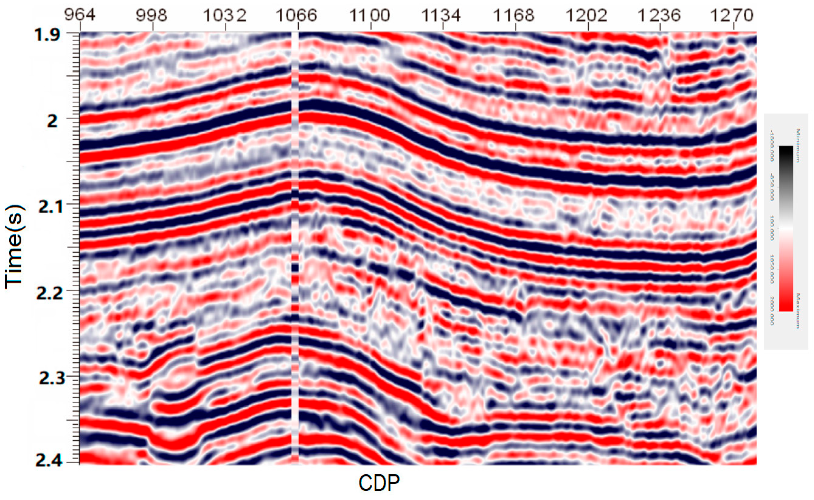
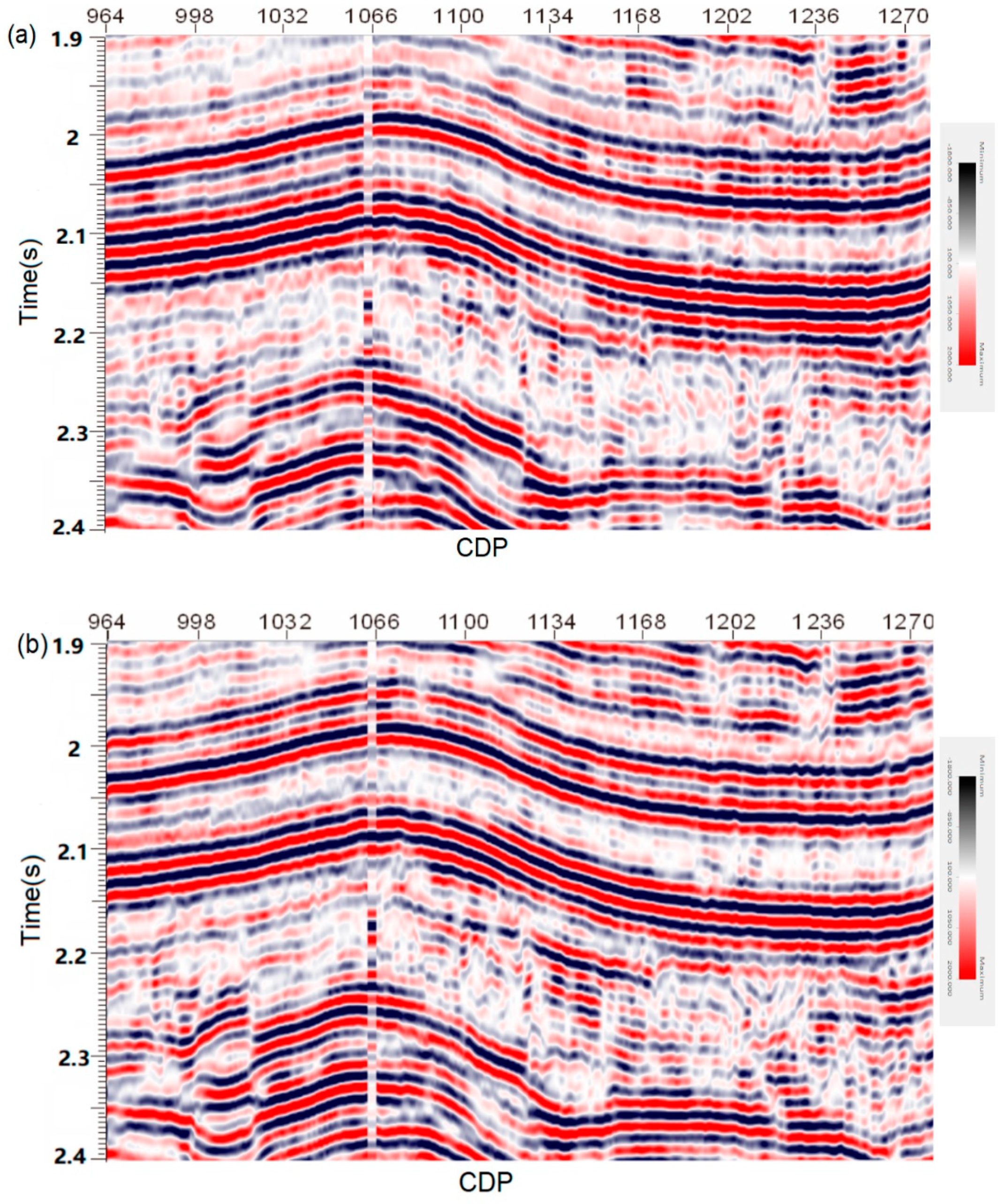
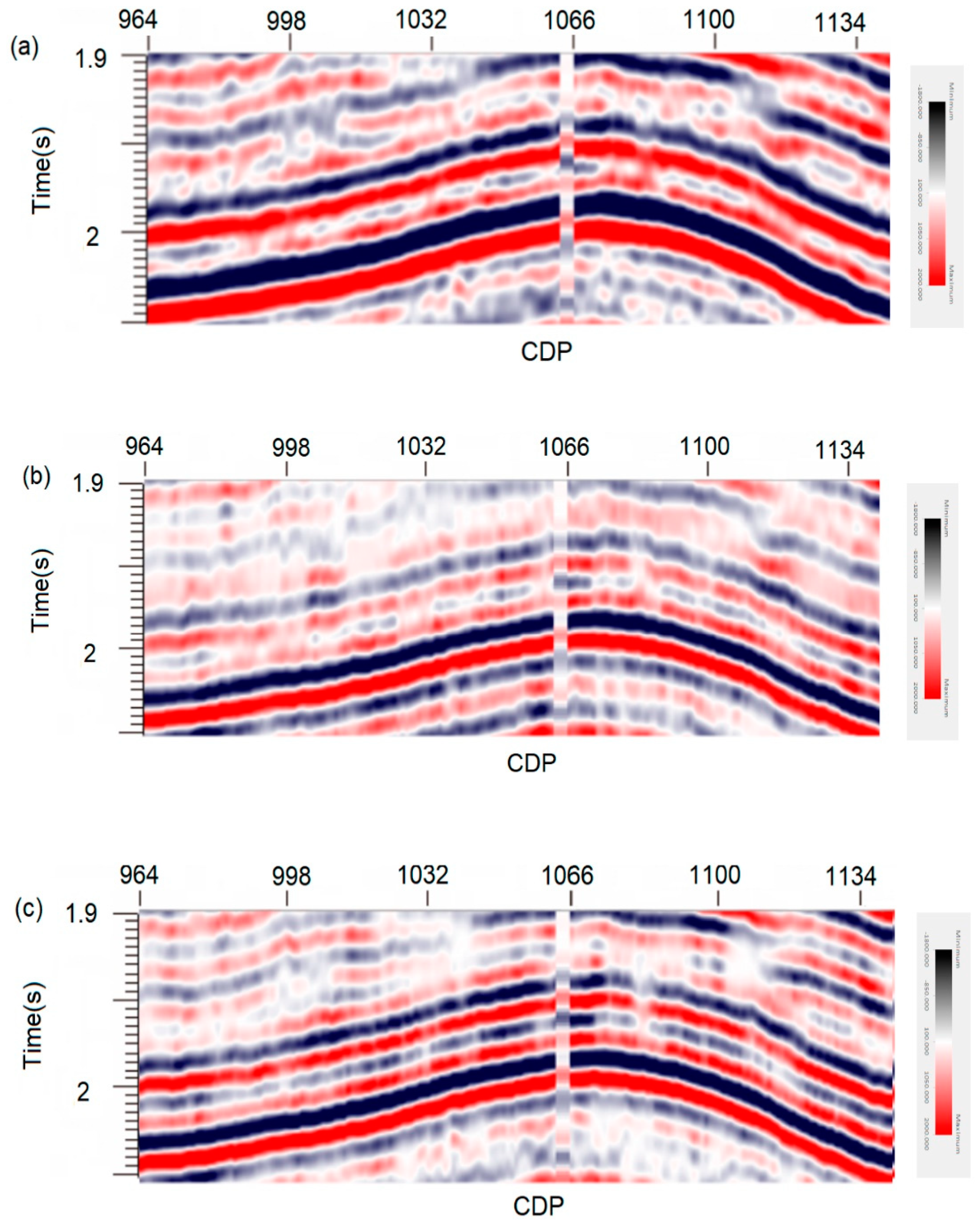
5. Real Data Processing

In this paper, seismic data of Yanmuxi in Thuha Basin are selected to test the applicability of the algorithm. Figure 12 shows the selected data corresponding to line 299, within the time interval of 1900 to 2400 ms. The resolution of these data is relatively low, which greatly hinders accurate seismic interpretation.

We use traditional ISTA algorithm and RNN-like ISTA deconvolution algorithm to process the seismic data with high resolution in order to improve the resolution of seismic data. We first need to generate the training data set, as mentioned above. We randomly generate 500 reflection coefficients, according to the rule of Gauss distribution. Subsequently, we generate a series of seismic wavelets with different frequencies and different phases. Finally, the training data set can be obtained by convoluting these seismic wavelets with reflection coefficients separately. Through training, we can get the RNN-like ISTA network related to seismic wavelet. Subsequently, we use this network to deconvolute Figure 12. Figure 13 shows the processing results. This figure shows that, after processing the seismic data by conventional ISTA and RNN-like ISTA, the number of data alignments in both seismic sections clearly increased when compared to the original data, which proves that the two algorithms provide higher resolution seismic data.

However, zoomed views of the same portion of the previous sections (Figure 14) allow for better appreciating the location of the seismic reflectors delineated by the two algorithms tested here. It can be seen that, when error backpropagation is applied (Figure 14c), the improved algorithm provides clearer seismic wavelets and, therefore, better structural details than the conventional algorithm (Figure 14b). The zones outlined by rectangles allow appreciating the gain in the definition of some markers. Analogously, the comparison of time slices at 2000 ms also demonstrates that the algorithm proposed in this study increases the resolution in the entire working area (Figure 15). Therefore, ISTA type RNN provides more suitable seismic information for a successful interpretation of the available real data.

6. Conclusions

We propose a sparse spike deconvolution algorithm that is based on an RNN-like ISTA. It is possible to obtain an alternative procedure that is similar to the RNN deep learning method by transforming the objective function of conventional ISTA. By applying the BPTT algorithm of an RNN, the backward correction of the involved method parameters during the iteration process can be performed. After multiple backward corrections, reasonable seismic wavelets were obtained, which were difficult to accurately determine. The use of the improved wavelet matrix to perform deconvolution allows for obtaining high resolution results. The analyses carried out with synthetic and real data demonstrate that the algorithm proposed in this study is able to increase the resolution of seismic data and that the processing efficiency of this algorithm is better than that of the conventional algorithm.

References

1. Mallat, S.G.; Zhang, Z. Matching pursuits with time-frequency dictionaries. IEEE Trans. Signal Process. 1993, 41, 3397–3415. [Google Scholar] [CrossRef] [Green Version]
2. Cai, T.T.; Wang, L. Orthogonal matching pursuit for sparse signal recovery with noise. IEEE Trans. Inf. Theory 2011, 57, 4680–4688. [Google Scholar] [CrossRef]
3. Chen, S.; Donoho, D.L.; Saunders, M.A. Atomic decomposition by basis pursuit. Siam J. Sci. Comput. 1998, 20, 33–61. [Google Scholar] [CrossRef]
4. Donoho, D.L. Compressedsensing. IEEE Trans. Inf. Theory 2006, 52, 1289–1306. [Google Scholar] [CrossRef]
5. Mairal, J.; Bach, F.; Ponce, J.; Sapiro, G. Online dictionary learning for sparse coding. In Proceedings of the 26th Annual International Conference on Machine Learning, Montreal, QC, Canada, 14–18 June 2009; pp. 689–696. [Google Scholar]
6. Beck, A.; Teboulle, M. A fast iterative shrinkage-thresholding algorithm for linear inverse problems. Siam J. Imaging Sci. 2009, 2, 183–202. [Google Scholar] [CrossRef] [Green Version]
7. Graves, A.; Mohamed, A.R.; Hinton, G. Speech recognition with deep recurrent neural networks. In Proceedings of the IEEE International Conference on Acoustics. Speech and Signal Processing, Vancouver, BC, Canada, 26–30 May 2013; Volume 38, pp. 6645–6649. [Google Scholar]
8. Lecun, Y.; Bengio, Y.; Hinton, G. Deep learning. Nature 2015, 521, 436–444. [Google Scholar] [CrossRef] [PubMed]
9. Schmidhuber, J. Deep learning in neural networks: An overview. Neural Netw. 2015, 61, 85–117. [Google Scholar] [CrossRef] [PubMed] [Green Version]
10. Pineda, F.J. Generalization of back-propagation to recurrent neural networks. Phys. Rev. Lett. 1987, 59, 2229–2232. [Google Scholar] [CrossRef] [PubMed]
11. Werbos, P.J. Backpropagation through time: What it does and how to do it. Proc. IEEE 1990, 78, 1550–1560. [Google Scholar] [CrossRef] [Green Version]
12. Kasać, J.; Deur, J.; Novaković, B.; Kolmanovsky, I. A conjugate gradient-based BPTT-like optimal control algorithm. In Proceedings of the IEEE International Conference on Control Applications, Petersburg, Russia, 8–10 July 2009; pp. 861–866. [Google Scholar]
Figure 1. Scheme of the iteration with iterative shrinkage-thresholding algorithm (ISTA).
Energies 13 03074 g001
Figure 2. Basic structure and operating scheme of a recurrent neural network (RNN).
Energies 13 03074 g002
Figure 3. RNN-like ISTA flow charts.
Energies 13 03074 g003
Figure 4. Flowchart of forward calculation using the improved ISTA.
Energies 13 03074 g004
Figure 5. Flowchart of the backward error correction algorithm.
Energies 13 03074 g005
Figure 6. (a) Zero-phase Ricker wavelets of frequencies 30, 40, and 50 Hz. (b) Noise-free seismic channel containing 512 sampling points and six reflection spikes. (c) Synthetic seismogram.
Energies 13 03074 g006
Figure 7. Training seismic data: (a) Ricker wavelets of different frequencies (10 Hz, 20 Hz, …, 70 Hz); (b) synthetic seismograms.
Energies 13 03074 g007
Figure 8. Comparison of the deconvolution results obtained by the algorithm proposed in this study (red spikes) and conventional ISTA (blue spikes).
Energies 13 03074 g008
Figure 9. Synthetic seismogram contaminated by noise (SNR = −4.55 dB).
Energies 13 03074 g009
Figure 10. Comparison of the deconvolution results obtained from the trial noisy seismogram by the algorithm proposed in this study (red spikes) and conventional ISTA (blue spikes).
Energies 13 03074 g010
Figure 11. Comparison of the convergence rate curves by the algorithm proposed in this study and conventional ISTA.
Energies 13 03074 g011
Figure 12. Field data extracted from well T3 (corresponding to the exploration line 299) located in the northern area of Yanmuxi in the Turpan Basin, west of China (data provided by courtesy of SINOPEC).
Energies 13 03074 g012
Figure 13. (a) Seismic section showing the deconvolution results after applying: (a) conventional ISTA; (b) the algorithm proposed in this study.
Energies 13 03074 g013
Figure 14. Enlarged views of the same portions of the previous sections that allow appreciate the location of the seismic reflectors delineated by the tested algorithms: (a) real field data; (b) image recovered by conventional ISTA; and, (c) section processed by the algorithm proposed in this study.
Energies 13 03074 g014
Figure 15. Time slices at 2000 ms that show the deconvolution results obtained: (a) from the original data; (b) by the algorithm proposed in this study; and, (c) by conventional ISTA.
Energies 13 03074 g015