Numerical Simulation of the Flow in a Kaplan Turbine Model during Transient Operation from the Best Efficiency Point to Part Load ^†

Abstract

The aim of this study is to develop a reliable numerical model that provides additional information to experimental measurements and contributes to a better exploitation of hydraulic turbines during transient operation. The paper presents a numerical analysis of the flow inside a Kaplan turbine model operated at a fixed runner blade angle during load variation from the best efficiency point (BEP) to part load (PL) operation. A mesh displacement is defined in order to model the closure of the guide vanes. Two different types of inlet boundary conditions are tested for the transient numerical simulations: linear flow rate variation (InletFlow) and constant total pressure (InletTotalPressure). A time step analysis is performed and the influence of the time discretization over the fluctuating quantities is discussed. Velocity measurements at the corresponding operating points are available to validate the simulation. Spectrogram plots of the pressure signals show the times of appearance of the plunging and rotating modes of the rotating vortex rope (RVR) and the stagnation region developed around the centerline of the draft tube is captured.

1. Introduction

Nowadays, hydropower plants are experiencing frequent off-design operation regimes and load variations because of the fluctuating energy production requirements. The energy market is becoming more dynamic due to its deregulation in some countries, as well as the introduction of intermittent renewable energy sources, such as wind and solar power [1]. Transient operations induce pressure oscillations and asymmetric loads on the runner blades of hydraulic turbines, affecting their lifetime, increasing the pressure losses and reducing the efficiency of the power plants [2]. Furthermore, closing the guide vanes, i.e., reducing the flow entering the turbine, results in a high swirl at the runner outlet of single-regulated turbines, leading to the formation of the rotating vortex rope (RVR) [3]. In the draft tube of the turbine, the RVR generates large amplitude pressure fluctuations at low frequencies in the range of 0.2–0.4 × f_runner, where f_runner represents the runner rotational frequency. It is therefore necessary to accurately predict the RVR formation in order to avoid the unfavorable operation of hydraulic turbines. The analysis of the vortex formation and its mitigation may allow for the development of effective countermeasures. Both experimental and numerical techniques have been used for such investigations.

Experimental studies of the pressure fluctuations inside hydraulic machines were carried out for different operating points during steady and transient operations [4,5,6]. The measurements showed that the largest amplitudes of the pressure fluctuations were attained during transient operations, especially during total or partial load rejection. The formation and mitigation of the RVR in the draft tubes of hydraulic machines were investigated experimentally during part load (PL) operation [7,8]. The study of a Francis turbine model during load decrease focusing on the RVR formation [3] showed that at a low guide vane angle, i.e., low flow rate, the runner was unable to extract the high swirl provided by the guide vanes. As a consequence, a highly swirling flow entered the draft tube and the axial velocity increased near the draft tube walls. Due to the large pressure gradient in the radial direction, the radial component of the velocity was negative near the draft tube walls. A recirculation region was observed behaving as a blockage to the draft tube flow leading to the formation of the RVR. The rotating vortex was showed to wrap around the high pressure/low velocity areas.

Computational fluid dynamics (CFD) is becoming a powerful tool in modelling turbulent flows and acquiring information concerning the operation of hydraulic machines [9,10,11]. Numerical simulations are now a faster and more cost-efficient alternative to experimental investigations and model testing. However, there are still limitations in turbulence modelling regarding the space and time discretization, the definition of boundary conditions and the modelling of the Reynolds Averaged Navier–Stokes (RANS) equations [12]. Furthermore, in order to model transient flows in hydraulic turbines, a mesh displacement method should be employed [13], thus increasing the complexity of the numerical model, and the total simulation time. A good compromise between the accuracy of the simulation and the limited computational resources is challenging to achieve.

Transient numerical models of load variation in hydraulic turbines require the modelling of the guide vanes displacement using a time dependent space discretization. In the case of double-regulated turbines, a moving mesh is required for the runner blades as well. Various moving mesh methods have been employed for different industrial applications, such as the movement of the junction between the airplane tail and the fuselage [14] or free surface flows [15]. A transient numerical model of a pump-turbine was developed using a dynamic mesh method and re-meshing techniques in order to model the flow during load rejection [16]. Concerning hydraulic turbines, there are only a few studies available in the literature. An axial turbine was investigated during sudden load rejection [17] using transient simulations and a moving mesh. Reference [18] presented the results of 3D unsteady RANS (URANS) simulations of the flow through a Francis turbine during load rejection and runaway transient operations. A study of load changes and complete shutdown of a Francis turbine model was presented in [19]. The guide vanes displacement was modelled using a mesh motion procedure and an automated re-meshing technique.

The inlet boundary conditions were proven to have a strong influence on the accuracy of numerical simulations regarding hydraulic turbines [20,21]. Different solutions to model the start-up of Francis turbines were investigated [22], showing the necessity of including the draft tube and the full runner domains in the numerical model. The authors considered a constant total pressure value as inlet boundary condition to simulate the flow through a Francis turbine model during start-up. The flow was underestimated in the numerical simulation due to an overestimation of the losses. URANS simulations of the flow inside a bulb draft tube were performed [23], discussing the accuracy of the inlet boundary conditions required in order to correctly capture the flow features. The simulations underestimated the velocity values in the draft tube domain due to the overestimation of the head losses, especially near the draft tube walls.

The numerical investigations performed to model the pressure fluctuations exerted on the runner blades are predominantly URANS simulations of different operating regimes [24,25,26]. Several researchers carried out numerical simulations attempting to describe and explain the RVR formation. It was found that the use of the k-epsilon turbulence model for such studies is not recommended, as the swirl is underestimated and the vortex is strongly damped [27]. The Scale-Adaptive Simulation- Shear Stress Transport (SAS-SST) turbulence model was employed in unsteady simulations of the flow inside the draft tube of a Kaplan turbine during PL operation [28]. The authors were able to capture the RVR movement and showed that the turbulence model provides results in good agreement with the experimental values.

In recent years, a lot of focus has been dedicated to the investigation of the transient operation of Francis-type turbines. However, the number of studies aiming to investigate Kaplan turbines is limited.

The objective of our research is to create and validate a transient numerical model of a Kaplan turbine operated on a propeller curve, i.e., at a fixed runner blade angle. The paper is an extension of a previous study [29], after the improvement of the geometrical accuracy of the model. Transient URANS simulations of the flow through a Kaplan turbine model are carried out to investigate the flow behavior during the partial closure of the guide vanes, i.e., load variation from best efficiency point to part load operation. The guide vanes displacement is modelled using a moving mesh defined as specified displacement relative to the initial position. Two types of inlet boundary conditions are considered: a linear flow variation and a constant total pressure. The numerical results are compared to velocity and pressure measurements in the runner and draft tube. The selection of the boundary conditions and the influence of the time step definition over the accuracy of the numerical model are discussed. A time step sensitivity analysis is performed aiming to obtain a good accuracy of the results while maintaining low computational resources and a relatively short simulation time. The RVR formation during the guide vane closure is investigated. Spectrograms of the pressure on the runner blades and on the draft tube cone wall are presented showing the time of appearance of the RVR plunging and rotating modes.

2. Materials and Methods

2.1. Test Case

The Porjus U9 Kaplan turbine model [30] is numerically investigated. The turbine includes a spiral casing, a distributor (18 stay vanes and 20 guide vanes), a 6-blade runner, and an elbow draft tube. The runner diameter is 0.5 m and the rotational speed is 696.3 rpm. The turbine model was investigated experimentally during steady operation at the best efficiency point (BEP) and off-design operation points [30,31,32]. The experimental results are used for the validation of the numerical model.

Velocity and pressure measurements were presented in [3,6,30,31,32]. Six pressure sensors were used on the pressure side of one runner blade and six on the suction side of the neighboring runner blade, as illustrated in Figure 1.

In the upper part of the draft tube cone, 20 pressure sensors were used (Figure 2a) located at four angular positions a, b, c and d (Figure 2b) according to [30].

Laser Doppler Anemometry (LDA) measurements were performed in the runner chamber [32] and in the draft tube cone [30]. The velocity profiles are presented along one radius (direction d, Figure 2b) as the results are similar in the other directions. The numerically simulated velocity components are recorded by 20 monitor points defined along the blue lines presented in Figure 3. The line corresponding to Section I (Figure 3) is extended and the velocity and pressure values are recorded along the diameter of the draft tube cone in an attempt to capture the asymmetric flow developed during load rejection and PL operation.

The transient simulations are validated with the corresponding stationary operating condition measurements at the BEP and PL.

Transient pressure measurements during load variations on the Porjus U9 model were also carried out [6]. The load variations were performed on a propeller curve, i.e., at a fixed runner blade angle, but the total head value was not constant as the experiment was performed in a close loop circuit. The total head (H) of the turbine is defined as:

$$H=\frac{p_1-p_2}{\rho g}+\frac{Q^2}{2g}\cdot \left(\frac{1}{A_1^2}-\frac{1}{A_2^2}\right)+z_1-z_2$$

(1)

where the indexes 1 and 2 represent the inlet of the guide vane domain and the outlet of the draft tube, respectively.

The transient operation of the Porjus U9 turbine from the BEP to PL is modelled. The average angular velocity of the guide vane closing is ω_GV = 0.859°/s and the total time of the load variation is Δt = 7.57 s. The main parameters for the BEP and PL operating points are presented in

Table 1. Operating condition parameters of the Porjus U9 model. Experimental values.

Operating Point	BEP	PL
αGV (°)	26.5	20
Q (m3/s)	0.69	0.62
H (m)	7.5	7.5

.

2.2. Numerical Model

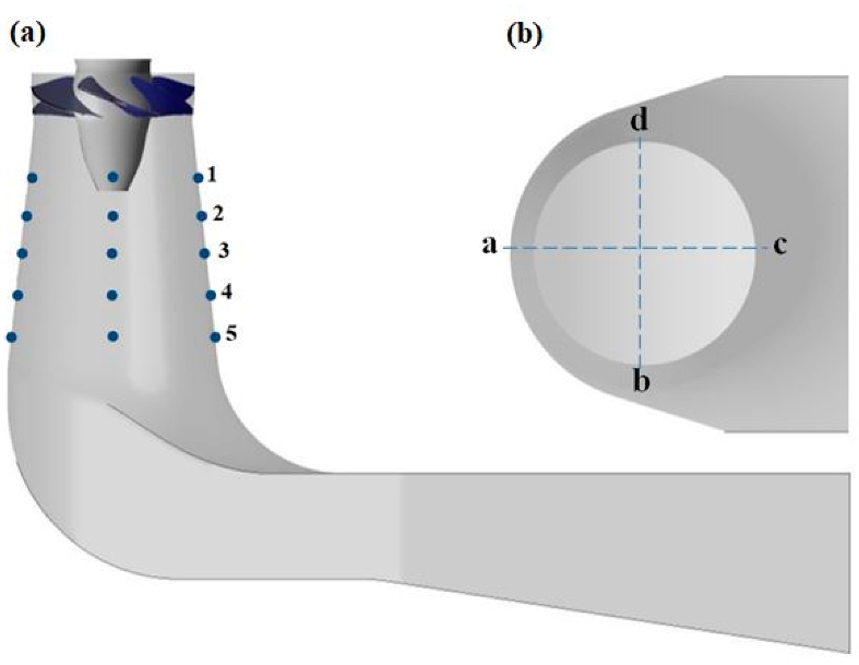
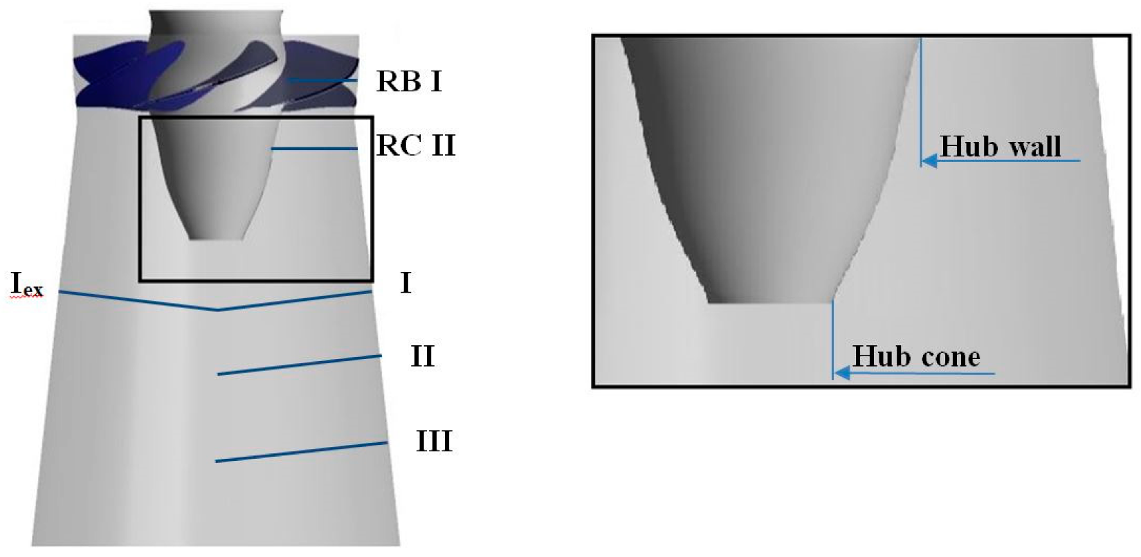
2.1.1. Analysis Domain

The numerical simulations were performed for the Porjus U9 turbine model using the CFX Ansys solver. The numerical model includes one moving guide vane, the complete runner with six runner blades, and the elbow draft tube (Figure 4). The model was developed considering the results published in [22,33], concerning the influence of the domain selection over the accuracy of the numerical simulations. The draft tube domain includes the draft tube cone, elbow, and diffuser. A single guide vane is modelled and a Stage interface is defined between the guide vane domain and the runner domain. The advantage of such interfaces is that the pitch change is modelled by taking the circumferential averages over circular bands along the interface. However, the downside of the Stage interface is that the velocity profile is averaged before entering the downstream component. Therefore, blade wakes and pressure fluctuations are damped. At the draft tube inlet, a Transient Rotor–Stator interface is used in order to capture the transient relative motion and the frame change between the runner and the draft tube. The simulations are performed using the k-ω SST turbulence model. The k-ω SST turbulence model is selected for providing a reasonable precision at low computational costs [34]. The computational resources are a particularly important aspect when modelling transient flows with mesh displacement.

2.1.2. Mesh

A hexahedral unstructured mesh is created for each computational domain using the software ICEM 16.2. A single runner blade passage is discretized. The mesh is multiplied and rotated in order to attain certain axial symmetry of the flow inside the runner domain. The total number of cells in the Kaplan turbine model is 13.96 × 10⁶. The mesh quality criteria are presented in

Table 2. Quality parameters of the mesh used in the transient simulations.

Domain	No. of Elements (×106)	Minimum Angle (°)	Expansion Factor (–)	Aspect Ratio (–)	y+ (min/avg/max) (–)
Guide vane	0.34	20.2	16	58	2.70/15.6/27.1
Runner	9.96	16.8	48	668	0.90/15.7/67.0
Draft tube	3.66	30.5	9	7635	0.02/1.12/4.40

.

A mesh sensitivity study for the guide vanes, runner and draft tube of the Porjus U9 turbine model was carried out [35]. In the current study, the guide vane and runner domains are discretized similarly, attempting to improve the mesh quality and decrease the y⁺ values. The size of the guide vane mesh is comparable to the previous version, but the runner domain mesh is refined.

Using a hexahedral mesh can be rather restrictive in terms of mesh quality. The aim was to create a good quality mesh instead of a fine mesh with low quality. The y⁺ values presented in Table 2 are, in some areas, larger than the recommended value of 1; therefore, the automatic wall function is locally employed in the CFX simulations [36]. This automatic wall treatment switches between the wall function approach and the low Re approach (k-ω) depending on the grid spacing near the wall [37]. A very fine mesh, that meets the y⁺ <1 criterion, considerably increases the mesh size, the computational demands and the total simulation time.

The mesh displacement is defined for the guide vane computational domain. The guide vane rotates around the center of rotation C (x_c, y_c) shown in Figure 5. The location of the guide vane blade (x_t, y_t) is calculated at each time step using coordinates relative to the previous mesh position (x_t−1, y_t−1):

$$xt=(xt-1-xc)\cos (d\alpha GV)+(yt-1-yc)\sin (d\alpha GV)+xc$$

(2)

$$yt=(yt-1-yc)\cos (d\alpha GV)-(xt-1-xc)\sin (d\alpha GV)+yc$$

(3)

where x_t and y_t are the coordinates of the guide vane blade at the current time step, x_t−1 and y_t−1 are the coordinates of the guide vane blade at the previous time step and x_c and y_c are the coordinates of the center of rotation.

The guide vane angle (dα_GV), related to the initial position, is calculated at each time step (dt) as:

$$d\alpha GV=\omega GV\cdot dt\cdot n$$

(4)

where n is the current time step.

2.1.3. Boundary Conditions

Concerning the modelling of transient load variations of hydraulic turbines, the inlet boundary conditions may be provided as velocity (volumetric flow rate, mass flow or velocity profiles) or pressure (static or dynamic). It was proven that using the linear flow variation as an inlet boundary condition leads to an inaccurate prediction of the pressure variation [19]. The study concluded that the total pressure should be defined at the inlet and the flow variation should be obtained from the simulations. The use of these two types of inlet boundary conditions is investigated in the present paper: the linear variation of the flow rate (referred to as: InletFlow simulation) and a constant total pressure value during the load variation (referred to as: InletTotalPressure simulation). In the following sections, the variables with the index Q or P will refer to the InletFlow and InletTotalPressure simulations, respectively.

It is recommended for the time step (dt) to be selected considering the smallest frequency of the system to be resolved. Usually, a time step corresponding to 1° ÷ 5° of the runner angular rotation is chosen. In the present case, this would correspond to a sampling frequency of 2092 to 836.8 Hz. With such a time step size, part of the turbulent fluctuations are resolved from the lowest turbulent frequency, which is about V/D ≈ 8 Hz (where V is the average velocity of the flow at the runner inlet and D is the characteristic length, in the present case, the runner diameter) up to half of the sampling frequency. From our experience and the literature [38], the use of small time step values may cause the simulation to overpredict the pressure/velocity fluctuations. In this case, the overestimations most likely occur due to the URANS equations resolving part of the turbulence, which they are not designed for. RANS models are statistical representations of the turbulent flow. They are not designed to resolve part of the turbulence as the large eddy simulation (LES) model is.

2.1.4. Time Step Sensitivity Analysis

A time step sensitivity analysis is performed for three different time step sizes, as presented in

Table 3. Time step sensitivity analysis.

Case	Time Step dt [s]	Corresponding Runner Rotation dθ (°)
1	0.001195	5
2	0.014579	61
3	0.028919	121

. The large time step values corresponding to large angles of the runner rotation (dθ = 61° and 121°) are employed because the flow delivered to the runner is axis-symmetric, all six runner blades are identical, and the inlet into the draft tube cone is axis-symmetric as well. Considering all the above, a time step corresponding to 61° of the runner rotation should be equivalent to a time step corresponding to 1°. The sampling frequencies are 68.6 and 35.6 Hz, and part of the turbulence is still resolved. The largest time step size allows for resolving the RVR with at least 15 points per RVR rotation (1 RVR rotation ≈ 5 runner rotations). All simulations are carried out using the high-resolution scheme for the advection term and the second order backward Euler scheme for the time-dependent terms in the URANS equations.

First, a steady-state simulation of the flow in the turbine model operated during BEP operation is performed in order to obtain the initial conditions for the transient simulations. The mass flow rate is defined at the inlet of the guide vane domain. The computed total head is further used for the InletTotalPressure simulation in order to start with a similar flow rate compared to the InletFlow simulation.

Secondly, URANS simulations are performed for 15 runner rotations (1.3 s) during BEP operation followed by the guide vane closure. At the end of the guide vane closure (Δt = 7.57 s), the simulations continue for another 83 runner rotations (7.2 s) to ensure the convergence and stabilization of the flow parameters at PL. The total simulated time is approximately 16 s for both types of inlet boundary conditions, i.e., mass flow rate and constant total pressure.

The inlet boundary condition InletTotalPressure is used to test the hypothesis of axis-symmetric flow developed in the runner domain and large time steps: 61° and 121°.

3. Results and Discussion

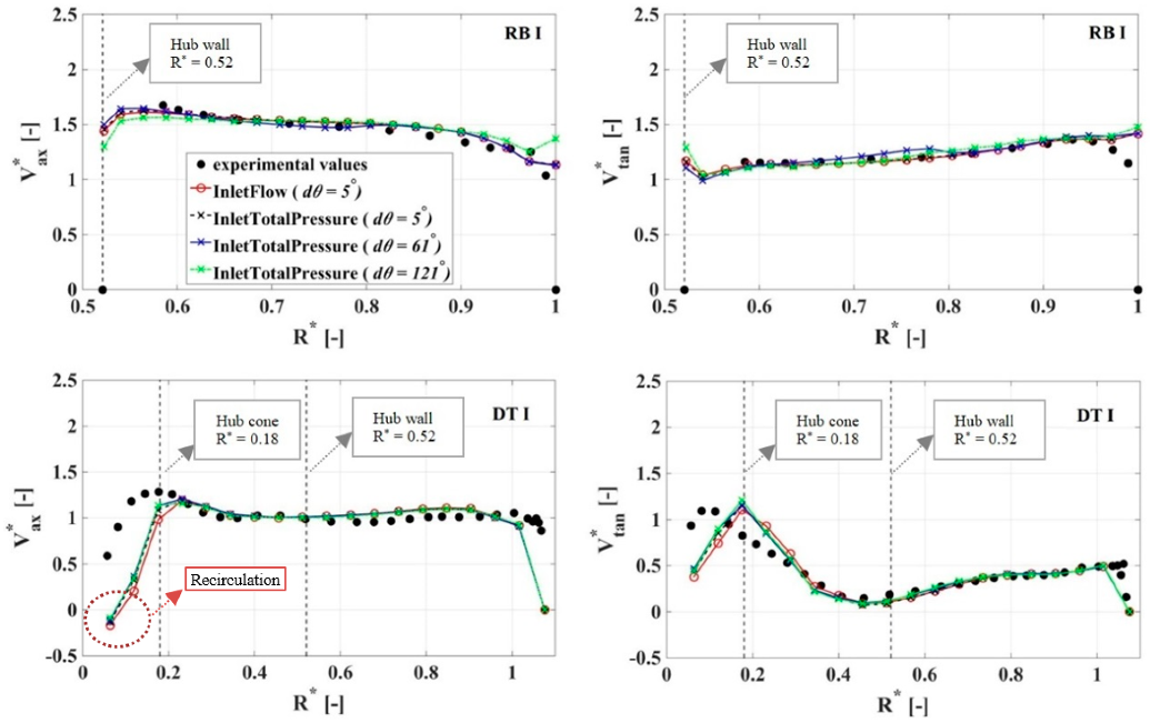
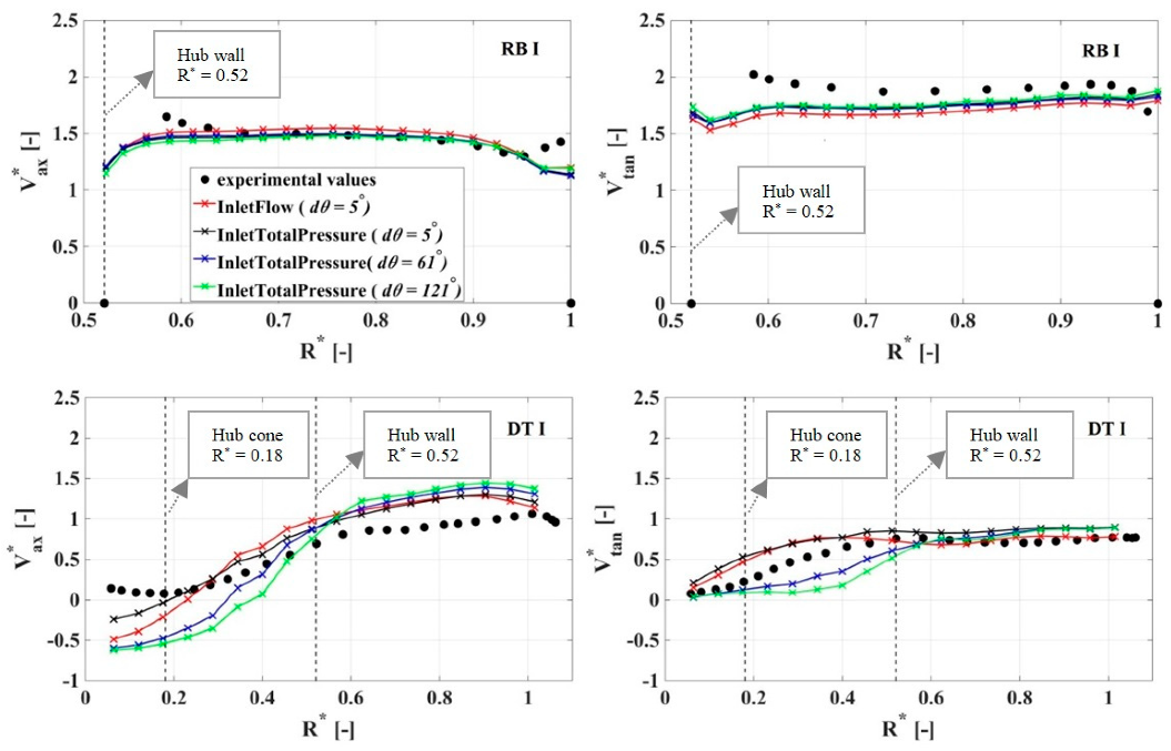
3.1. Validation with Experimental Velocity Profiles

The numerical results are validated using velocity measurements. The results of the steady-state simulations before (BEP) and after (PL) the transient simulation are compared to experimental profiles. The results are presented in Figure 6 for Section RB I, in the runner domain and Section I in the draft tube domain (see Figure 3). All the velocity values are normalized with the bulk velocity calculated from the flow rate and the area corresponding to the runner diameter. The radii are made dimensionless relative to the runner radius R = 0.25 m. The positive direction in the runner and draft tube cone for the axial velocity is vertically downward, along the Z axis as presented in Figure 4.

The BEP velocity profiles are obtained by averaging the numerical results over 15 runner rotations, whereas the PL velocity profiles are averaged over 80 ÷ 83 runner rotations (depending on the time step value). When using the small time step size dθ = 5° of the runner rotation, it is possible to average only over the last period, e.g., the last runner rotation given that enough samples are provided. Assuming the results are converged, this is the recommended procedure. However, if the large time step sizes are used, i.e., dθ = 61° and 121°, one runner rotation provides only six or three samples, respectively, and it is not enough to calculate a representative mean value. Therefore, the average over all the runner rotations simulated was chosen to obtain the mean velocity profiles.

In the runner blade channel (Section RB I) at the BEP, the numerical model provides reasonable results compared to the measurements regardless of the inlet boundary conditions (Figure 6). The velocity profiles show that the flow is following the geometry of the runner blade with boundary layers developing on the hub and shroud in the axial and tangential direction. However, below the runner hub (DT I section), in the center of the draft tube cone (R* < 0.25), the flow is difficult to model accurately. The axial jets formed in the blade-hub clearances are not captured in the simulations. This is due to the turbulence model overpredicting the swirl leaving the runner domain, i.e., the tangential velocity is overestimated near the axis of the draft tube and the axial velocity is underestimated showing negative values. The overestimation of the tangential velocity is certainly related to the underestimation of the axial velocity and an inadequate modelling of the clearances (insufficient number of cells, large y⁺ values). Therefore, the simulations show a recirculation area formed at the inlet of the draft tube, even during BEP operation. The different time steps have a marginal effect on the runner and no effect on the draft tube as the velocity profiles overlap on a single profile.

During PL operation, the flow angle provided by the guide vanes at the inlet of the runner domain is far from the design conditions. Secondary flows occur, and the turbulent fluctuations are increasing in amplitude because of the RVR formation in the draft tube of the turbine [23]. Therefore, numerical simulations have difficulties in matching the experimental results (Figure 7). In the runner domain, Section RB I, the simulations show a slight sensitivity to the inlet boundary conditions, but no influence from the time step size. On the other hand, considerable differences are obtained in the draft tube domain just below the runner hub, between the numerical simulations (influenced by both the time step size and the initial boundary conditions) and the experimental measurements. For a constant time step size, the inlet boundary condition has a small influence. However, the InletTotalPressure simulation predicts considerably different velocity profiles depending on the time step size.

3.2. Inlet Boundary Conditions

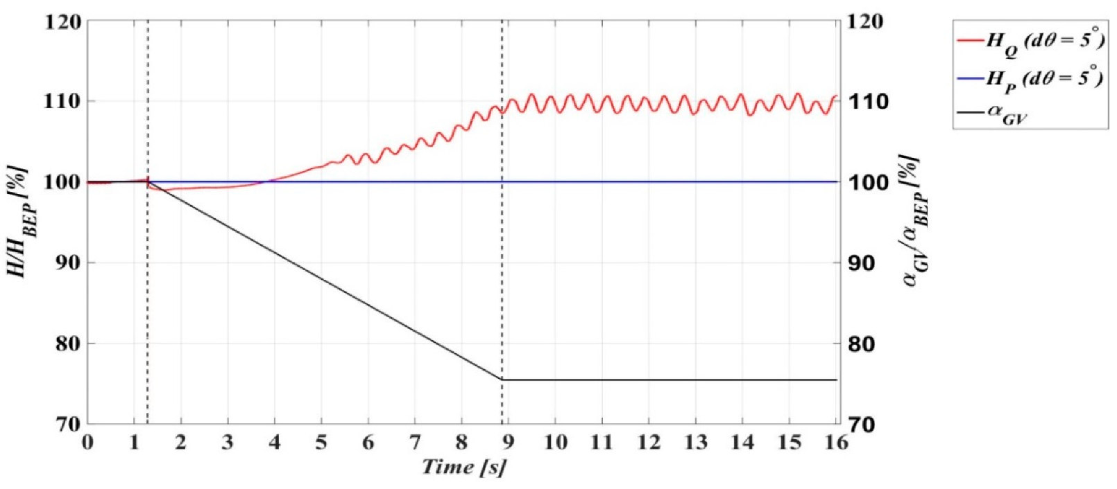
3.2.1. Main Parameters

The influence of the inlet boundary conditions, i.e., linear flow variation (InletFlow simulation) and constant total pressure (InletTotalPressure simulation), is presented and discussed. The numerical values of the main parameters (Q and H) obtained from the two transient simulations (InletFlow and InletTotalPressure) are compared.

First, the BEP operation of the turbine is modelled, i.e., the steady-state initial condition (approximately 1.3 s). During the load variation (Δt = 7.57 s), the guide vane rotates with Δα_GV = 6.5° and PL operation is reached.

Figure 8 presents the time variation of the flow rate (Q) simulated using the two different inlet boundary conditions. The results of the simulations employing the smallest time step (dt = 0.001195 s or dθ = 5°) are presented in order to compare similar set-ups. The flow rate values are normalized with the numerically obtained flow rate during BEP operation. In the case of the InletFlow simulation, the value coincides with the flow rate measured by Amiri et al. (2016a). The results of the InletFlow simulation are considered the reference in Figure 8 since the linear variation of the flow rate (Q_Q) is specified at the inlet of the guide vane domain according to the experiment. Using the total constant pressure as the inlet boundary condition leads to an underestimation of the flow rate (Q_P) by approximatively 3% during PL operation. The influence of the different boundary conditions over the variation of the parameters becomes visible around t = 4 s. The results confirm that the head losses are overestimated by the turbulence model. The justification for this overestimation is that the head losses are predominantly due to turbulent kinetic energy dissipation [23], hence being overestimated by URANS models. Another possible cause may be the wall function used in the numerical simulations for y⁺ > 1 [39]. The turbulent fluctuations are overpredicted, and the energy losses are large, especially near the solid boundaries. However, resolving the boundary layers up to y⁺ = 1 would result in a too large number of hexahedral cells to perform calculation in a reasonable amount of time.

The time variation of the simulated total head (H) is presented in Figure 9. Like the previous plot, the values are normalized with the head obtained at the BEP from the simulations. Despite defining a numerically obtained head value as the inlet boundary condition, the results of the InletTotalPressure show an underestimation of the flow rate from the middle of the transient at t = 4 s, as seen in Figure 8. On the other hand, the head is overestimated by the InletFlow simulations at PL, approximately 10% over the BEP constant value. As expected, the numerical model is over predicting the head required to maintain the fixed flow rate despite the high pressure losses. The overestimation of the pressure losses is due to the turbulence modelling, and the use of wall functions implied by the coarse mesh. The head solution begins to diverge approximately 4 s after the beginning of the simulations, similar to the flow rate variation.

The simulations were carried out for different time step sizes and it was shown that the time step size has a marginal influence over the numerical head and flow rate values [40]. It can be concluded that the main flow parameters of a turbine during transient operation can be modelled using larger time step values based on the assumption that the flow is axis-symmetric inside the turbine. Both computational resources and simulation time can thus be reduced using large time steps.

3.2.2. Pressure Oscillations

Figure 10 presents the pressure signal variation recorded numerically at a monitor point located near the leading edge on the pressure side of the blade (PS1, Figure 3) and the corresponding pressure measured at the BEP. The influence of the different inlet boundary conditions becomes noticeable. In the runner domain, the InletFlow simulation predicts a quasi-constant relative pressure during the load decrease, as opposed to the InletTotalPressure simulation. The measurements carried out during the transient operation captured a descending trend of the pressure signal [2] similar to the results of the InletTotalPressure simulation. Such results are expected from the fixed flow rate simulation where an overestimation of the pressure losses is observed in the analysis of the main parameters (Q and H) as well. The oscillations resulting from the RVR formation (to be discussed) in the draft tube are also different; the amplitude is larger for the InletFlow simulation.

Further downstream, at a monitor point located on the draft tube cone wall (3c, Figure 4), the influence of the boundary conditions is no longer visible in the average pressure prediction (Figure 11). However, the amplitude of the pressure fluctuations obtained with the InletTotalPressure simulation is larger than those obtained with the InletFlow simulation. The time interval between two consecutive pressure peaks is approximately 0.45 s corresponding to a dimensionless frequency of 0.19 × f_runner.

In order to investigate the RVR formation, the accurate prediction of the velocity profiles and the pressure fluctuations inside the draft tube cone is necessary [3]. Due to the overestimation to the pressure losses, the InletTotalPressure simulations underestimate the flow rate and the InletFlow simulations overestimate the head. Regardless, the velocity profiles seem insensitive to the inlet boundary conditions. The pressure variation is, however, captured more accurately by the InletTotalPressure simulation (Figure 10). Therefore, from this section on, only the results of the InletTotalPressure simulation are discussed.

The amplitude of the pressure fluctuations is strongly influenced by the time step size. As the time step size decreases, the amplitudes of the simulated pressure fluctuations increase. Small time steps may induce the prediction of larger amplitudes of the pressure/velocity fluctuations than the experimental values. On the other hand, when large time steps are used, a larger part of turbulence is modelled as opposed to it being resolved. In this case, the dissipative RANS turbulence models are expected to under-predict the fluctuations compared to the experiments.

Figure 12 presents the frequency domain analysis of the simulated pressure monitored at the locations on the runner blade (PS1) and the draft tube wall (3c) for all time step values. The Fast Fourier Transform (FFT) is employed. The frequency is normalized using the runner rotational frequency, f_runner = 11.61 Hz. All simulations show amplitude peaks at approximately the same dimensionless frequencies. Their amplitude is, however, strongly influenced by the time step size.

As presented in [3,6], the RVR can be decomposed into two modes: synchronous and asynchronous. The simulations capture both the synchronous (f/f_runner = 0.19) and the asynchronous mode of the RVR (f/f_runner = 0.81) on the runner, corresponding to the two largest amplitude peaks captured in Figure 12a. The lower peaks represent the harmonics of the two modes. Figure 12b shows that the monitor point located on the draft tube wall, in the stationary frame of reference, still captures the same frequency of 0.19 × f_runner and its harmonics. The results confirm the experimental values reported in [6,31].

The influence of the time step size is not visible in the average velocity profiles, nor the time evolution of the main parameters (Q and H), showing that large time step sizes may be used to capture the main flow features. However, when analysing the pressure fluctuations, this influence becomes substantial. From this section on, only the results of the InletTotalPressure simulation employing the smallest time step are discussed.

3.3. Rotating Vortex Rope

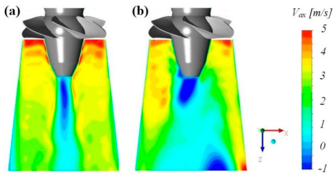
3.3.1. Flow Structure

In this section, the analysis of the load variation is carried out focusing on the RVR developed inside the Kaplan turbine model.

As the guide vanes close and the turbine operating point shifts from the BEP to PL, in the upper part of the draft tube the axial velocity distribution becomes asymmetrical (Figure 13). A gradual decrease of the flow rate leads to low axial velocity and larger tangential velocity at the runner outlet. The runner is not able to extract the swirl provided by the guide vanes at a low angle. As the flow rate decreases below a critical value, a low axial velocity region is formed near the centerline of the draft tube. The tangential component of the velocity becomes dominant and the flow is pulled towards the draft tube walls. Consequently, the flow is concentrated near the walls of the draft tube as shown in Figure 13b. The RVR rotates in the draft tube and in the core of the vortex a recirculation area develops. A circumferential circulation is generated at the draft tube inlet and an eccentric vortex rope is formed, wrapping around low velocity areas and rotating in the same direction as the runner.

Figure 14 presents the fully developed RVR during PL operation illustrated by means of an iso-pressure contour. The tangential velocity contours plotted at Sections I to III show how the RVR leads to the appearance of both a local minimum and a local maximum velocity. In the maximum velocity area, the tangential velocity is positive. This area represents the bulk swirling flow. In the low velocity areas near the axis of the draft tube, the tangential velocity becomes negative.

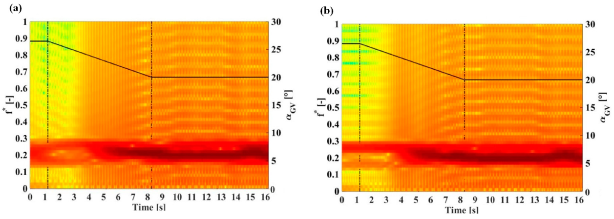
3.3.2. Spectral Analysis

In order to analyse the RVR formation and decomposition, spectrogram plots of the pressure fluctuations in the draft tube and on the runner blade recorded during the transient operation of the Kaplan turbine model are presented. The axial velocity distribution in the upper part of the draft tube is analysed as well.

To obtain the plunging (synchronous) and rotating (asynchronous) modes of the RVR [41], two pressure signals monitored at locations 3a,c (symmetrical to the draft tube centerline, Figure 2a) are analysed. The values of the two components presented in Figure 15 are determined according to Equations (5) and (6).

$$P_{pl}=\frac{P_{3a}+P_{3c}}{2}$$

(5)

$$P_{rot}=\frac{P_{3a}-P_{3c}}{2}$$

(6)

After subtracting the mean value, the signals are filtered using a second-order Savitzky–Golay filter to remove the background noise (Figure 15b). The filtered signal is used for the full spectrum spectrograms. In order to obtain the low frequency spectrograms, a pass band filter was applied to the signal within the limits of f_inf = 0.15 × f_runner and f_sup = 0.25 × f_runner (Figure 15c).

Figure 16 presents the spectrogram plot for the pressure signal monitored on the runner blade, near the leading edge on the pressure side of the blade (monitor point PS1) during the transient simulation. The other monitor points showed similar pressure variations and therefore are not presented. All the spectrograms presented in the paper are obtained using Matlab. The function provides the short-time Fourier transform of the signal. The signal is divided into a number of segments (windows) that overlap according to the user specifications.

Before the beginning of the guide vane closure, at t = 1.3 s, the only significant frequency is the one corresponding to the runner rotational frequency. Decreasing the flow rate leads to the RVR formation in the draft tube of the turbine. The pressure fluctuations induced by the vortex can be decomposed in a synchronous mode (or the plunging mode) and an asynchronous mode (or the rotating mode). It was shown that the plunging mode of the RVR produces pressure fluctuations at a frequency corresponding to approximately 0.2 × f_runner [6]. The pressure fluctuations caused by the RVR rotating mode have a frequency of 0.8 × f_runner in the rotating frame of reference, i.e., the runner.

Figure 16 shows that the two RVR components are captured by the pressure sensor located on the pressure side of the runner blade. The plunging mode component appears 4 s after the beginning of the guide vane closure (approximately t = 5.3 s). The frequency of the pressure fluctuations captured by the numerical simulation is f_pl = 0.2 × f_runner. The spectrogram shows that, in the runner rotating domain, the rotating component appears 1 s later than the plunging component at the dimensionless frequency of f_rot = 0.8 × f_runner.

Spectrograms of the plunging and rotating modes of the RVR for the pressure sensors located on the draft tube cone wall (3a,c, Figure 2a) are presented in Figure 17. In the draft tube stationary domain, the strongest amplitude is obtained at approximately 0.2 × f_runner in both cases. However, the time of appearance is not clear. The resolution of the spectrograms is, of course, influenced by the total number of samples and the sampling frequency corresponding to the simulation time step.

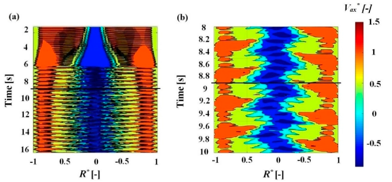
3.3.3. Decomposition of the Rotating Vortex Rope

The contour of the normalized axial velocity (V_ax*) monitored during the transient simulation is presented in Figure 18 starting from the beginning of the guide vane closure (t = 1.3 s). The velocity was recorded using 39 monitor points defined along the diameter of the draft tube cone (Section I and I_ex, Figure 5). The velocity values are normalized with respect to the bulk velocity at this section, calculated from the flow rate. The contour plot starts at t = 1.3 s, corresponding to the end of the BEP steady-state simulation (Figure 18a).

Although it is expected to obtain a uniformly distributed flow at the runner outlet at the BEP, the numerical simulation shows a small low velocity region under the runner hub (R* = ±0.07) (Figure 18a). As the flow rate decreases, the stagnation zone becomes wider. The axial velocity shows a strong negative gradient leading to an increase in the radial velocity component as the flow is pulled towards the draft tube walls. Approximately 5 s after the transient operation begins, the velocity field starts to oscillate. The fluctuations are initially formed only at the interface between the stagnation area and the bulk flow swirling toward the draft tube wall (Figure 18a). At PL, the velocity shows large period fluctuations along the entire diameter of the draft tube cone (Figure 18b).

Figure 19 presents the axial component of the velocity vectors during the transient simulation. The formation and the evolution of the RVR are illustrated at different time steps. At t = 4.2 s (corresponding guide vane angle: α_GV = 22.9°) the stagnation region is developing along the centerline of the draft tube. Just below the runner hub, the velocity values are negative. The RVR is already formed at t = 6.6 s and the bulk flow is visibly pushed towards the walls. By the end of the transient operation, at t = 8.87 s, the RVR is wrapped around the low velocity areas.

4. Conclusions

Transient URANS simulations of the flow through the Porjus U9 Kaplan turbine model were carried out aiming to investigate the limitations of the CFD modelling of transient phenomena and evaluate faster simulation strategies. The computational domain included one moving guide vane, six fixed runner blades and the draft tube. The selected test case was the load variation from BEP to PL operation.

The influence of two types of inlet boundary conditions (linear flow variation and constant total pressure) on the precision of transient simulations was discussed. When the linear flow rate variation was provided as the inlet condition, the simulations overpredicted the head values by approximatively 10% due to the numerical overestimation of the pressure losses. If, however, the total pressure was provided, the flow rate was underestimated by up to 3%. The velocity profiles were accurately predicted in the runner and draft tube compared to the experiments, regardless of the type of inlet boundary conditions used.

A time step sensitivity analysis was carried out, and the pressure fluctuations recorded on the runner blade were studied in order to select a time step value that provided the best precision of the results. A small time step value will lead to larger amplitude fluctuations of the simulated pressure values. Simulations using very large time steps will, on the other hand, only obtain mean values of the fluctuating quantities with significantly smaller amplitude. However, the main parameters of the flow (head and flow rate) are captured accurately regardless of the time step size. The influence of the time discretization over the prediction of the velocity profiles is also small and inconsistent.

In order to test the validated numerical model, the RVR formation inside the Kaplan turbine draft tube was investigated. The stagnation region that leads to the vortex breakdown was visible in the axial velocity contours plotted in the runner and draft tube domains. Spectrograms of the pressure signals recorded on the runner blades and the draft tube walls were presented. The frequency of the runner blade passing (6 × f_runner) and its harmonics were captured by all monitor points. The plunging and rotating modes of the pressure fluctuations induced by the RVR were also visible in the spectrograms. The plunging mode component was captured by the numerical simulation approximately 4 s after the start of the guide vane closure at f_pl = 0.2 × f_runner. The spectrogram of the pressure monitored on the runner blade showed that the rotating component appeared 1 s later at the dimensionless frequency of f_rot = 0.8 × f_runner. The numerical results were similar to the values determined experimentally [6].

The study explored the limitations of CFD simulation in modelling transient turbulent flows in hydraulic turbines. The pressure losses are overestimated given the coarse computation of the near-wall flows with large pressure gradients, complex geometry and strong curvature. Achieving a good compromise between the computational demands and the accuracy of the numerical simulations is also a challenge.

References

1. Banshwar, A.; Sharma, N.K.; Sood, Y.R.; Shrivastava, R. Market based procurement of energy and ancillary services from renewable energy sources in deregulated environment. Renew. Energy 2017, 101, 1390–1400. [Google Scholar] [CrossRef]
2. Amiri, K.; Cervantes, M.J.; Mulu, B. Experimental investigation of the hydraulic loads on the runner of a Kaplan turbine model and the corresponding prototype. J. Hydraul. Res. 2015, 53, 452–465. [Google Scholar] [CrossRef]
3. Goyal, R.; Cervantes, M.J.; Gandhi, B.K. Vortex rope formation in a high head model Francis turbine. J. Fluids Eng. 2017, 139, 041102. [Google Scholar] [CrossRef]
4. Houde, S.; Fraser, R.; Ciocan, G.; Deschênes, C. Experimental study of the pressure fluctuations on propeller turbine runner blades: Part 2, transient conditions. IOP Conf. Ser. Earth Environ. Sci. 2012, 15, 062061. [Google Scholar] [CrossRef] [Green Version]
5. Chirag, T.; Cervantes, M.J.; Bhupendrakumar, G.; Dahlhaug, O.G. Pressure measurements on a high-head Francis turbine during load acceptance and rejection. J. Hydraul. Res. 2014, 52, 283–297. [Google Scholar] [CrossRef]
6. Amiri, K.; Mulu, B.; Raisee, M.; Cervantes, M.J. Unsteady pressure measurements on the runner of a Kaplan turbine during load acceptance and load rejection. J. Hydraul. Res. 2016, 54, 1–18. [Google Scholar] [CrossRef]
7. Ciocan, G.D.; Iliescu, M.S.; Vu, T.C.; Nennemann, B.; Avellan, F. Experimental study and numerical simulation of the FLINDT draft tube rotating vortex. J. Fluids Eng. 2006, 129, 146–158. [Google Scholar] [CrossRef]
8. Favrel, A.; Müller, A.; Landry, C.; Yamamoto, K.; Avellan, F. Study of the vortex-induced pressure excitation source in a Francis turbine draft tube by particle image velocimetry. Exp. Fluids 2015, 56. [Google Scholar] [CrossRef]
9. Lipej, A.; Čelič, D.; Tartinville, B.; Mezine, M.; Hirsch, C. Reduction of CPU time for CFD analysis of hydraulic machinery development process. IOP Conf. Ser. Earth Environ. Sci. 2012, 15, 62011. [Google Scholar] [CrossRef] [Green Version]
10. Židonis, A.; Aggidis, G. State of the art in numerical modelling of Pelton turbines. Renew. Sustain. Energy Rev. 2015, 45, 135–144. [Google Scholar] [CrossRef]
11. Trivedi, C.; Cervantes, M.J. State of the art in numerical simulation of high head Francis turbines. Renew. Energy Environ. Sustain. 2016, 1, 20. [Google Scholar] [CrossRef] [Green Version]
12. Denton, J.D. Some limitations of turbomachinery CFD. In Proceedings of the ASME Turbo Expo 2010: Power for Land, Sea, and Air, Glasgow, UK, 14–18 June 2010; pp. 735–745. [Google Scholar] [CrossRef]
13. Tang, T. Moving mesh computations for computational fluid dynamics. Contemp. Math. 2005, 383, 141–173. [Google Scholar] [CrossRef] [Green Version]
14. Matsushima, K.; Murayama, M.; Nakahashi, K. Unstructured dynamic mesh for large movement and deformation. In Proceedings of the 40th AIAA Aerospace Sciences Meeting & Exhibit, Reno, NV, USA, 14–17 January 2002. [Google Scholar] [CrossRef]
15. Perot, J.B.; Nallapati, R. A moving unstructured staggered mesh method for the simulation of incompressible free-surface flows. J. Comput. Phys. 2003, 184, 192–214. [Google Scholar] [CrossRef]
16. Liu, J.; Liu, S.; Yuekun, S.; Yulin, W.; Leqin, W. Three dimensional flow simulation of load rejection of a prototype pump-turbine. Eng. Comput. 2013, 29, 417–426. [Google Scholar] [CrossRef]
17. Kolšek, T.; Duhovnik, J.; Bergant, A. Simulation of unsteady flow and runner rotation during shut-down of an axial water turbine. J. Hydraul. Res. 2006, 44, 129–137. [Google Scholar] [CrossRef]
18. Li, J.; Yu, J.; Wu, Y. 3D unsteady turbulent simulations of transients of the Francis turbine. IOP Conf. Ser. Earth Environ. Sci. 2010, 12, 012001. [Google Scholar] [CrossRef]
19. Mössinger, P.; Jester-Zürker, R.; Jung, A. Francis-99: Transient CFD simulation of load changes and turbine shutdown in a model sized high-head Francis turbine. J. Phys. Conf. Ser. 2017, 782, 12001. [Google Scholar] [CrossRef] [Green Version]
20. Gagnon, J.-M.; Flemming, F.; Qian, R.; Deschênes, C.; Coulson, S. Experimental and numerical investigations of inlet boundary conditions for a propeller turbine draft tube. In Proceedings of the ASME 2010 3rd Joint US-European Fluids Engineering Summer Meeting, Montreal, QC, Canada, 1–5 August 2010. [Google Scholar] [CrossRef]
21. Nilsson, H.; Cervantes, M.J. Effects of inlet boundary conditions, on the computed flow in the Turbine-99 draft tube, using OpenFOAM and CFX. IOP Conf. Ser. Earth Environ. Sci. 2012, 15, 32002. [Google Scholar] [CrossRef] [Green Version]
22. Nicolle, J.; Giroux, A.M.; Morissette, J.F. CFD configurations for hydraulic turbine startup. IOP Conf. Ser. Earth Environ. Sci. 2014, 22, 32021. [Google Scholar] [CrossRef]
23. Wilhelm, S.; Balarac, G.; Métais, O.; Ségoufin, C. Analysis of head losses in a turbine draft tube by means of 3D unsteady simulations. Flow Turbul. Combust. 2016, 97, 1255–1280. [Google Scholar] [CrossRef] [Green Version]
24. Nicolet, C.; Arpe, J.; Avellan, F. Identification and modelling of pressure fluctuations of a Francis turbine scale model at part load operation. In Proceedings of the IAHR 22nd Symposium on Hydraulic Machinery and Systems, Stockholm, Sweden, 29 June–2 July 2004. [Google Scholar]
25. Liu, S.; Li, S.; Wu, Y. Pressure fluctuation prediction of a model Kaplan turbine by unsteady turbulent flow simulation. J. Fluids Eng. 2009, 131, 101102. [Google Scholar] [CrossRef]
26. Wu, Y.; Liu, S.; Dou, H.-S.; Wu, S.; Chen, T. Numerical prediction and similarity study of pressure fluctuation in a prototype Kaplan turbine and the model turbine. Comput. Fluids 2011, 56, 128–142. [Google Scholar] [CrossRef]
27. Ruprecht, A.; Helmrich, T.; Aschenbrenner, T.; Scherer, T. Simulation of vortex rope in a turbine draft tube. In Proceedings of the Hydraulic Machinery and Systems 21st IAHR Symposium, Lausanne, Switzerland, 9–12 September 2002. [Google Scholar]
28. Maddahian, R.; Cervantes, M.J.; Sotoudeh, N. Numerical investigation of the flow structure in a Kaplan draft tube at part load. IOP Conf. Ser. Earth Environ. Sci. 2016, 49, 22008. [Google Scholar] [CrossRef] [Green Version]
29. Iovănel, R.G.; Bucur, D.M.; Dunca, G.; Cervantes, M.J. Numerical analysis of a Kaplan turbine model during transient operation. IOP Conf. Ser. Earth Environ. Sci. 2019, 240, 022046. [Google Scholar] [CrossRef]
30. Mulu, B.; Jonsson, P.; Cervantes, M.J. Experimental investigation of a Kaplan draft tube—Part I: Best efficiency point. Appl. Energy 2012, 93, 695–706. [Google Scholar] [CrossRef]
31. Jonsson, P.; Mulu, B.; Cervantes, M.J. Experimental investigation of a Kaplan draft tube—Part II: Off-design conditions. Appl. Energy 2012, 94, 71–83. [Google Scholar] [CrossRef]
32. Amiri, K.; Mulu, B.; Cervantes, M.J. Experimental investigation of the interblade flow in a Kaplan runner at several operating points using Laser Doppler Anemometry. J. Fluids Eng. 2015, 138, 021106. [Google Scholar] [CrossRef]
33. Melot, M.; Nennemann, B.; Désy, N. Draft tube pressure pulsation predictions in Francis turbines with transient Computational Fluid Dynamics methodology. IOP Conf. Ser. Earth Environ. Sci. 2014, 22, 32002. [Google Scholar] [CrossRef] [Green Version]
34. Alfonsi, G. Reynolds-averaged Navier–Stokes equations for turbulence modeling. Appl. Mech. Rev. 2009, 62, 040802. [Google Scholar] [CrossRef]
35. Mulu, B.G.; Cervantes, M.J.; Devals, C.; Vu, T.C.; Guibault, F. Simulation-based investigation of unsteady flow in near-hub region of a Kaplan Turbine with experimental comparison. Eng. Appl. Comput. Fluid Mech. 2015, 9, 1–18. [Google Scholar] [CrossRef] [Green Version]
36. Menter, F.; Carregal-Ferreira, J.; Esch, T.; Konno, B. The SST turbulence model with improved wall treatment for heat transfer predictions in gas turbines. In Proceedings of the International Gas Turbine Congress, Tokyo, Japan, 2–7 November 2003. [Google Scholar]
37. Ansys 16.2 Documentation CFX Modelling guide 4.2. Modelling Flow Near the Wall. 2014. Available online: http://http://read.pudn.com/downloads500/ebook/2077964/cfx_mod.pdf (accessed on 12 June 2020).
38. Trivedi, C.; Cervantes, M.J.; Dahlhaug, O.G. Experimental and numerical studies of a high-head Francis turbine: A review of the Francis-99 test case. Energies 2016, 9, 74. [Google Scholar] [CrossRef] [Green Version]
39. Nicolle, J.; Cupillard, S. Prediction of dynamic blade loading of the Francis-99 turbine. J. Phys. Conf. Ser. 2015, 579, 012001. [Google Scholar] [CrossRef] [Green Version]
40. Iovanel, R.G. Numerical Investigation of the Flow in a Kaplan Turbine. Ph.D. Thesis, Politehnica University of Bucharest, Bucharest, Romania, 2018. [Google Scholar]
41. Nishi, M.; Kubota, T.; Matsunaga, S. Surging characteristics of conical and elbow type draft tubes. In Proceedings of the 12th IAHR Symposium on Hydraulic Machinery, Equipment, and Cavitation, Stirling, Scotland, 27–30 August 1984. [Google Scholar]
Figure 1. Pressure sensors location on two consecutive runner blades. (a) PS1 to PS6 on the pressure side. (b) SS1 to SS6 on the suction side.
Energies 13 03129 g001
Figure 2. Pressure sensors location on the wall of the draft tube cone. (a) The positions are marked by blue dots. (b) Circumferential positions.
Energies 13 03129 g002
Figure 3. Locations of the velocity monitor points along the blue lines: Section RB (between the runner blades), Section RC (runner cone below the runner blades), Sections numbered I to III (in the draft tube cone), and Section Iex (the extension of Section I).
Energies 13 03129 g003
Figure 4. Computational domains and interfaces: 1. Guide vane and stay vane domain. 2. Guide vane–Runner interface. 3. Runner domain. 4. Runner–Draft tube interface. 5. Draft tube domain.
Energies 13 03129 g004
Figure 5. Spatial discretization of the guide vane domain at the beginning of the transient operation (BEP) and the end of the transient operation PL).
Energies 13 03129 g005
Figure 6. Experimental and simulated axial (Vax*) and tangential (Vtan*) velocity at the BEP, in the runner blade channel (Section RB I) and below the runner hub (Section DT I). The dotted vertical lines represent the hub wall and cone.
Energies 13 03129 g006
Figure 7. Experimental and simulated axial (Vax*) and tangential (Vtan*) velocity at PL, in the runner blade channel (Section RB I) and below the runner hub (Section DT I). The dotted vertical lines represent the hub wall and cone.
Energies 13 03129 g007
Figure 8. Time-dependent variation of the guide vane angle and discharge (Q) during the load variation. The dotted vertical lines represent the start and the end of the guide vane closure.
Energies 13 03129 g008
Figure 9. Time-dependent variation of the guide vane angle and head (H) during the load variation. The dotted vertical lines represent the start and the end of the guide vane closure.
Energies 13 03129 g009
Figure 10. Pressure–time variation (monitor point PS1 in the runner domain). The dotted horizontal line represents the mean pressure measured at the BEP. The dotted vertical lines represent the start and the end of the guide vane closure, respectively.
Energies 13 03129 g010
Figure 11. Pressure–time variation (monitor point 3c in the draft tube domain). The dotted horizontal line represents the mean pressure measured at the BEP. The dotted vertical lines represent the start and the end of the guide vane closure.
Energies 13 03129 g011
Figure 12. Amplitude spectra of the numerical pressure signal recorded throughout the load variation and PL operation. (a) Monitor point PS1 near the leading edge, on the pressure side of the blade. (b) Monitor point 3c on the draft tube cone wall.
Energies 13 03129 g012
Figure 13. Axial velocity (Vax) in the draft tube at (a) the BEP and (b) PL. Results of the InletTotalPressure simulation.
Energies 13 03129 g013
Figure 14. Iso-pressure contour of the rotating vortex rope (RVR) in the draft tube of a Kaplan turbine model during PL operation. Tangential velocity contours are presented for Sections I, II and III (see Figure 3).
Energies 13 03129 g014
Figure 15. (a) RVR components—raw signal. (b) Savitzky–Golay filtered pressure signal. (c) Truncated pressure signal. The y-scales are different for the three plots.
Energies 13 03129 g015
Figure 16. Spectrograms of the pressure monitor PS1 (runner blade, pressure side). (a) Full spectrum. (b) Low-frequency spectrum. The black solid line represents the guide vanes angle with the y-scale to the right. The dotted vertical lines represent the start and the end of the guide vane closure.
Energies 13 03129 g016
Figure 17. Spectrograms of the RVR plunging mode (a) and rotating mode (b). The black solid line represents the guide vanes angle with the y-scale to the right. The dotted vertical lines represent the start and the end of the guide vane closure.
Energies 13 03129 g017
Figure 18. Normalized axial velocity at Section I. (a) and detail around the end of the guide vane closure (b). The black horizontal line represents the ending of the transient operation.
Energies 13 03129 g018
Figure 19. Axial projection of the velocity vector field during load rejection, t = 1.3 s at the BEP (the beginning of the transient operation), t = 4.2 s and t = 6.6 s (during the guide vane closure), t = 8.87 s (the end of the transient operation), t = 16 s at PL.
Energies 13 03129 g019