Optimal Configuration of a Gas Expansion Process in a Piston-Type Cylinder with Generalized Convective Heat Transfer Law

Abstract

Optimal configurations for the working fluid expansion process in a piston-type cylinder with maximum work production are studied by applying finite time thermodynamics. The problem is solved by utilizing the modified Lagrangian. The initial and final volumes, initial internal energy and total time are fixed, and the heat transfer between the working fluid and the external heat bath obeys the generalized convective heat transfer law, which can be transformed into Newton’s heat transfer law, the Dulong–Petit heat transfer law and the square convective heat transfer law. The optimal configurations of the expansion process under three different conditions of heat transfer law are provided and compared, respectively. The results show that the heat transfer law has both quantitative and qualitative influences on the optimal configurations of the expansion process.

1. Introduction

Finite time thermodynamics (FTT) [1,2,3,4,5,6,7,8,9,10,11,12,13] has been applied to perform performance analyses and optimizations for various thermodynamic cycles and processes, including multi-stream heat exchange system [14], chemical reactors [15,16,17,18], electrochemical device [19], biological process [20], Novikov engines [21,22,23], Agrawal engine [24], Carnot engines [25,26], solar engine [27], internal combustion engine cycles [28,29,30,31,32], thermoelectric devices [33,34,35,36], cogeneration plants [37,38,39], ocean thermal energy conversion plants [40,41,42], Kalina cycle [43], Rankine cycles [44,45,46], Brayton cycles [47,48,49], Maisotsenko cycles [50,51], ratchet engine [52], electron engine [53] and the quantum engine [54]. It is one of the standard problems to determine the optimal configurations (OCs) for thermodynamic processes with the specific optimization objectives in FTT. To solve the OCs problems, Euler–Lagrange formalism and optimal control theory are two important methods. For some optimal control problems, analytic solutions can be derived. While for the other problems without analytic solutions, numerical methods are required to be referred. All thermodynamic parameters can be solved once the OCs are obtained. Therefore, it is more complex and significant to study the problems of OCs.

Many investigations about the OCs of different theoretical and practical engine models have been carried out by applying the Euler–Lagrange formalism or optimal control theory. Rubin [55,56] took account of Newton’s heat transfer law (NHTL) $q\propto \Delta (T)$ and took the maximum power production as the optimization objective to investigate the OCs of an endoreversible heat engines (HEs) under different constraint conditions. Ondrechen et al. [57] considered the change of heat-reservoir temperature and investigated the OC of the HE with NHTL. Adopting the similar heat transfer and heat reservoir models, Chen et al. [58] researched the heat leakage influence on the OC. Refs. [59,60,61,62] conducted studies on the optimal piston motions (OPMs) for the four-stroke Otto [59,60] and Diesel [61,62] cycle HEs with NHTL. Watowich et al. [63,64] carried out optimizations for light-driven dissipative engines with NHTL based on the maximum work output (MWP) and minimum entropy generation criteria, and obtained the optimal piston trajectories. Teh et al. [65,66] researched the optimal cycle of adiabatic internal combustion engine (ICE) under the condition of maximum efficiency by considering the heat leakage and chemical reaction loss as major losses of ICEs. Bi et al. [67] optimized the charging and discharging processes of the gas-hydrate with NHTL based on the minimum entropy generation criterion, and determined the OCs of the temperature and gas-hydrate phase change rate.

Band et al. [68,69] studied the optimal motion of a piston-type cylinder with NHTL based on the MWP criterion by using Euler–Lagrange ($E-L$) formalism, and obtained the OC of an ideal gas expansion process (EP), which consists of three phases as follows: (1) an adiabatic phase at the initial time; (2) an intermediate $E-L$ arc; (3) a final instantaneous adiabatic phase. Besides, the OCs of the EP with eight kinds of constraints were analyzed and compared. On the basis of Refs. [68,69], Band et al. [70] extended the obtained results to the external combustion engine in which the heat transfer obeys NHTL. Aizenbud and Band [71] and Salamon et al. [72] took the MWP [71] and the maximum power output [72] as optimization objectives to research the OCs of EP under the condition of NHTL, respectively. Based on the obtained results from Refs. [68,69], Aizenbud et al. [73] further studied the ICE model with NHTL.

Studying the effects of heat transfer laws (HTLs) on the OCs of thermodynamic processes and cycles is one of the most important works of FTT. In fact, heat transfer between the working fluid (WF) and external heat bath (EHB) does not always obey NHTL. There are many different HTLs, such as the linear phenomenological heat transfer law (LPHTL) $q\propto \Delta (T^{-1})$, radiative HTL $q\propto \Delta (T^4)$, Dulong–Petit heat transfer law (DPHTL) $q\propto {\left(\Delta T\right)}^{5/4}$, and the convective-radiative HTL $q\propto \Delta (T)+\Delta (T^4)$. Establishing the universal model and obtaining the universal laws and results are the aim of pursuing FTT, and that is the same for the OC studies. Beside the above simple HTLs, there are three universal HTLs: generalized radiative HTL (GRHTL) $q\propto \left(T^n-T_{ex}^n\right)$, generalized convective HTL (GCHTL) $q\propto {\left(T-T_{ex}^{}\right)}^n$ and the complex generalized HTL $q\propto {\left(T^n-T_{ex}^n\right)}^m$ which includes GRHTL and GCHTL. The HTL not only significantly affects the OCs of the thermodynamic processes with the specific optimization objectives, but also affects the performances of given thermodynamic processes. Refs. [74,75,76,77,78,79] took the MWP and the maximum efficiency as optimization objectives to determine the OCs of the endoreversible HEs with different constraints and different HTLs, including the LPHTL [74], radiative HTL [75,79] and GRHTL [76,77,78]. Yan et al. [80] researched the OC of a HE with variable-temperature heat reservoir and LPHTL based on the MWP criterion. Besides, some studies on the OCs of the HEs with GRHTL [81], GCHTL [82] and complex generalized HTL [83] under condition of variable-temperature heat reservoirs were conducted based on MWP criterion. Burzler and Hoffmann [84] and Burzler [85] adopted a four-stroke Diesel HE model and researched the OPM of the HE with the convective-radiative HTL under the condition of maximum power output. Xia et al. [86] obtained the OPM of an Otto cycle HE with the MWP under the condition of LPHTL. Ge et al. [87] considered both the NHTL and LPHTL, and optimized the minimum entropy generation to obtain the OPM of an Otto cycle. Ma et al. [88] introduced the LPHTL into a light-driven dissipative engine, and obtained the OPM of the engine with the MWP and minimum entropy generation.

On basis of Refs. [68,69], Refs. [89,90,91] concluded the OC for the EP of WF in a piston-type cylinder with the LPHTL [89], GRHTL [90] and convective-radiative HTL [91]. Moreover, Ref. [90] obtained the first-order approximate analytic solutions of the $E-L$ arcs by adopting Taylor series expansion when $n$ is equal to 2, 3 and 4. Chen et al. [92] further adopted the elimination method to study the intermediate $E-L$ arcs of the EP with the GRHTL, and obtained the analytic solutions when $n$ is equal to 2 and 3. Based on the obtained results in Ref. [89], Refs. [93,94] further investigated the external combustion engine [93] and the ICE [94] models with the LPHTL.

From the above introduction, one can see that, for a piston-type cylinder, lots of authors have studied the OCs under NHTL, LPHTL, radiative HTL, convective-radiative HTL and GRHTL. In Refs. [90,92], the utilized generalized radiative law $q\propto \left(T^n-T_{ex}^n\right)$ includes Newtonian $\left(T-T_{ex}\right)$, radiative $\left(T^4-T_{ex}^4\right)$, linear phenomenological $\left(T_{ex}^{-1}-T^{-1}\right)$, $\left(T^2-T_{ex}^2\right)$, $\left(T^3-T_{ex}^3\right)$ and other laws. It does not include some special laws, such as ${\left(T-T_{ex}^{}\right)}^2$, ${\left(T-T_{ex}^{}\right)}^3$, ${\left(T-T_{ex}^{}\right)}^{5/4}$. Therefore, in order to fully reveal the effects of HTLs on OCs and enrich FTT theory, the OCs under another generalized law, GCHTL $q\propto {\left(T-T_{ex}^{}\right)}^n$ should be studied. Based on Refs. [68,69,89,90,91,92], the OCs for the EP of WF in a piston-type cylinder will be studied using the modified Lagrangian in this paper. The initial and final volumes, initial internal energy and total time will be fixed, and the MWP with GCHTL $q\propto {\left(T-T_{ex}^{}\right)}^n$ will be obtained. The OCs of the EP under conditions of NHTL ($n=$ 1), DPHTL ($n=5/4$) and square convective heat transfer law (SCHTL) ($n=$ 2) will be provided and compared, respectively.

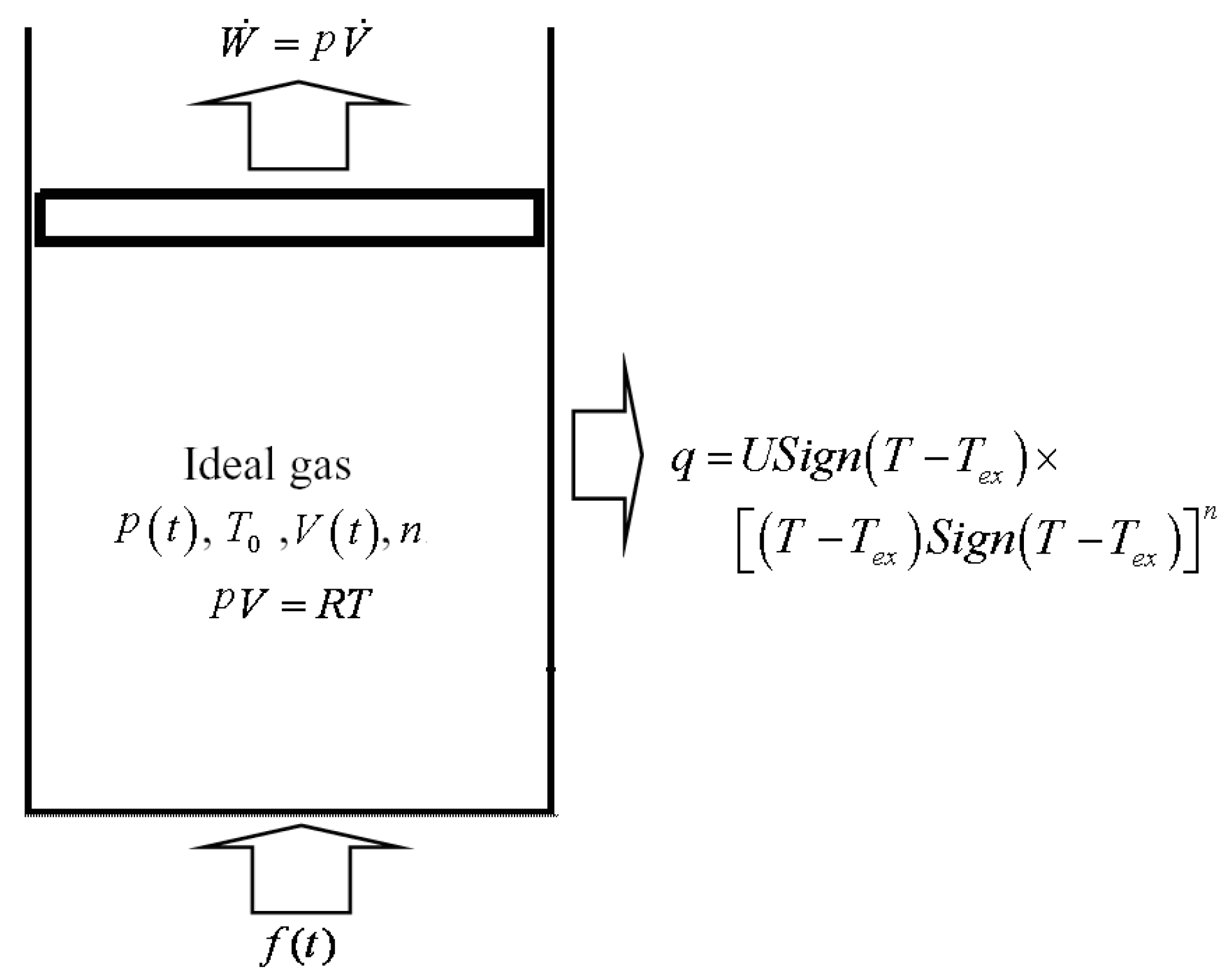
2. Modeling

Figure 1 shows a piston-type cylinder, in which an ideal gas expands to generate work. There are six assumptions: (1) the WF is an ideal gas and the mole number of WF is $1\mathrm{mol}$; (2) the ideal gas unevenly absorbs heat from the heat source, and the heat absorption rate is $f(t)$ that is an arbitrarily provided function about the time; (3) the EHB temperature $T_{ex}$ is constant, which the ideal gas can be coupled to; (4) the work generated from this system within a specified time interval can be furthest used by controlling the piston motion; (5) the inertias of the piston and the WF are negligible, and the friction loss due to the movement of the piston is also negligible; (6) the heat transfer obeys the GCHTL [82,95,96,97,98,99]. The heat conductance ($U$) of the cylinder wall is an important parameter for heat transfer, which is the product of the heat transfer coefficient and the contact area between the WF and cylinder. Nevertheless, this paper simplifies $U$ as a constant [68,69].

According to the first law of thermodynamics, for the thermal system shown in Figure 1, one has:

$$\dot{E}\left(t\right)=f\left(t\right)-\dot{W}\left(t\right)-U{\left[\left(T-T_{ex}\right)Sign\left(T-T_{ex}\right)\right]}^{n}Sign\left(T-T_{ex}\right)$$

(1)

where $\dot{E}\left(t\right)$ and $\dot{W}(t)$ are the change rate of the WF internal energy and WF expansion power, respectively. Besides, the sign function $\mathit{Sign}\left(T-T_{ex}\right)$ is equal to 1 as $T-T_{ex}\ge 0$ and -1 as $T-T_{ex}<0$.

Within the time internal $(0,t_m)$, the work ($W$) produced by the system due to the expansion of the heated WF is:

$$W={\displaystyle {\int }_0^{t_m}p(t)\dot{V}(t)dt}$$

(2)

where $t_m$ is the expansion time, $p$ is the WF pressure, and $V$ is the WF volume. According to Ref. [68], the process of irreversible efficiency ($\eta$) can be written as

$$\eta =W/\{E_p+R{T}_{ex}\ln [V_m/V(0)]\}$$

(3)

where $E_p$ is the WF absorbed energy, and it is equal to ${\displaystyle {\int }_0^{t_m}f(t)dt}$. Besides, $R{T}_{ex}\ln [V_m/V(0)]$ is the maximum energy obtained from the WF that expands from $V(0)$ to $V_m$ under the condition of an isothermal expansion temperature ($T_{ex}$).

3. Optimal Solutions

Taking the WF as an ideal gas, the relationships of $p\left(t\right)=RT\left(t\right)/V$ and $E\left(t\right)=C_{V}T\left(t\right)$ hold, where $R$ and $C_V$ are the gas constant and specific heat, respectively. The $p\left(t\right)=RE\left(t\right)/C_{V}V\left(t\right)$ can be obtained by combining above the relationships. Substituting it into Equations (1) and (2) yields:

$$\dot{E}\left(t\right)=f\left(t\right)-\frac{R}{C_V}E\left(t\right)\frac{\dot{V}\left(t\right)}{V\left(t\right)}-U{\left\{\left[E\left(t\right)/C_V-T_{ex}\right]Sign\left(T-T_{ex}\right)\right\}}^{n}Sign\left(T-T_{ex}\right)$$

(4)

$$W={\displaystyle {\int }_0^{t_m}\frac{R}{C_V}E\frac{\dot{V}\left(t\right)}{V\left(t\right)}dt}$$

(5)

The optimal control problem is:

$$\mathit{maximize}W={\displaystyle {\int }_0^{t_m}\frac{R}{C_V}E\frac{\dot{V}\left(t\right)}{V\left(t\right)}dt}$$

(6)

which is constrained by Equation (4).

For solving the above problem, the modified Lagrangian is established as following:

$$\begin{array}{ll}L=& \frac{R}{C_V}E\left(t\right)\frac{\dot{V}\left(t\right)}{V\left(t\right)}+\\ & \lambda \left(t\right)\left\{\dot{E}\left(t\right)-f\left(t\right)+\frac{R}{C_V}E\left(t\right)\frac{\dot{V}\left(t\right)}{V\left(t\right)}+U{\left\{\left[E\left(t\right)/C_V-T_{ex}\right]Sign\left(T-T_{ex}\right)\right\}}^{n}Sign\left(T-T_{ex}\right)\right\}\end{array}$$

(7)

where $\lambda (t)$ is the Lagrange multiplier for time. From Equation (7), one has:

$$\frac{\partial L}{\partial E}-\frac{d}{dt}\frac{\partial L}{\partial \dot{E}}=0,\frac{\partial L}{\partial V}-\frac{d}{dt}\frac{\partial L}{\partial \dot{V}}=0$$

(8)

The results of Equation (8) are first-order since the relationships between Lagrangian and $\dot{E}\left(t\right)$, and between Lagrangian and $\dot{V}\left(t\right)$ are linear. Hence, the arbitrary initial state and final state cannot be connected because the solutions have not sufficient free parameters. While the OPM can be composed by the motions contenting the Equation (8) and the motions on the accessible regional boundaries of the control variables, the motions contenting both the Equation (8) and adiabatic jumps must be combined together to derive the OPM because the boundary motions consist of infinitely adiabatic jumps [68].

Combining the modified Lagrangian with Euler–Lagrange equations, i.e., Equation (7) and Equation (8), the following equations can be obtained:

$$\dot{\lambda }\left(t\right)=\left[1+\lambda \left(t\right)\right]\frac{R}{C_V}\frac{\dot{V}\left(t\right)}{V\left(t\right)}+nU\lambda \left(t\right)\frac{{\left\{\left[E\left(t\right)/C_V-T_{\mathit{ex}}\right]\mathit{Sign}\left(T-T_{ex}\right)\right\}}^{n-1}}{C_V}$$

(9)

$$[1+\lambda (t)]\dot{E}(t)+\dot{\lambda }(t)E(t)=0$$

(10)

From Equations (4) and (9), one has:

$$\dot{E}=f\left(t\right)-\frac{E\left(t\right)\dot{\lambda }}{1+\lambda }+U{\left\{\left[E\left(t\right)/C_V-T_{\mathit{ex}}\right]Sign\left(T-T_{ex}\right)\right\}}^{n-1}\left\{\frac{E\left(t\right)\left[\left(n-1\right)\lambda \left(t\right)-1\right]}{\left[1+\lambda \left(t\right)\right]C_V}+T_{\mathit{ex}}\right\}$$

(11)

In the derivation of Equation (11), the following equation is used:

$${\left[Sign\left(T-T_{ex}\right)\right]}^{n+1}={\left[Sign\left(T-T_{ex}\right)\right]}^{n-1}\cdot {\left[Sign\left(T-T_{ex}\right)\right]}^2={\left[Sign\left(T-T_{ex}\right)\right]}^{n-1}$$

(12)

Combining Equation (10) with Equation (11) and eliminating $\dot{\lambda }(t)$ yields:

$$\lambda \left(t\right)=-\frac{\left[C_V{T}_{ex}-E\left(t\right)\right]\left\{U{\left\{\left[E\left(t\right)/C_V-T_{\mathit{ex}}\right]Sign\left(T-T_{ex}\right)\right\}}^n-f\left(t\right)Sign\left(T-T_{ex}\right)\right\}}{\begin{array}{l}U\left[\left(n-1\right)E\left(t\right)+C_V{T}_{ex}\right]{\left\{\left[E\left(t\right)/C_V-T_{\mathit{ex}}\right]Sign\left(T-T_{ex}\right)\right\}}^n+\\ f\left(t\right)\left[E\left(t\right)-C_V{T}_{ex}\right]Sign\left(T-T_{ex}\right)\end{array}}$$

(13)

Introducing the derivative of Equation (13) to the time, there is:

$$\dot{\lambda }\left(t\right)=\frac{\begin{array}{l}nU{\left\{\left[E\left(t\right)/C_V-T_{\mathit{ex}}\right]Sign\left(T-T_{ex}\right)\right\}}^n\{E\left(t\right)\dot{f}\left(t\right){\left[C_V{T}_{\mathit{ex}}-E\left(t\right)\right]}^{}Sign\left(T-T_{ex}\right)+\\ \dot{E}\left(t\right)\left\{U{C}_V{T}_{\mathit{ex}}{\left\{\left[E\left(t\right)/C_V-T_{\mathit{ex}}\right]Sign\left(T-T_{ex}\right)\right\}}^n+f\left(t\right)\left[nE\left(t\right)-C_V{T}_{\mathit{ex}}\right]Sign\left(T-T_{ex}\right)\right\}\}\end{array}}{\begin{array}{l}\{U\left[\left(n-1\right)E\left(t\right)+C_V{T}_{ex}\right]{\left\{\left[E\left(t\right)/C_V-T_{\mathit{ex}}\right]Sign\left(T-T_{ex}\right)\right\}}^n+\\ {f\left(t\right){\left[E\left(t\right)-C_V{T}_{ex}\right]}^{}Sign\left(T-T_{ex}\right)\}}^2\end{array}}$$

(14)

Substituting $\lambda \left(t\right)$ and $\dot{\lambda }\left(t\right)$, i.e., Equations (13) and (14), into Equation (11) yields:

$$\dot{E}\left(t\right)=\frac{\dot{f}\left(t\right)E\left(t\right)\left[C_V{T}_{\mathit{ex}}-E\left(t\right)\right]Sign\left(T-T_{ex}\right)}{\begin{array}{l}f\left(t\right)\left[{2C}_V{T}_{\mathit{ex}}-\left(n+1\right)E\left(t\right)\right]Sign\left(T-T_{ex}\right)-\\ \left[{2C}_V{T}_{\mathit{ex}}+\left(n-1\right)E\left(t\right)\right]U{\left\{\left[E\left(t\right)/C_V-T_{\mathit{ex}}\right]Sign\left(T-T_{ex}\right)\right\}}^n\end{array}}$$

(15)

According to Equation (15), the $E\left(t\right)$ with respect to $f\left(t\right)$ is solved. Moreover, the $V\left(t\right)$ of the WF is obtained by substituting $E\left(t\right)$ solved from Equation (15) into Equation (4) and then integrating over time.

$$\begin{array}{ll}V\left(t\right)=& V\left(0\right){\left[\frac{E\left(t\right)}{E\left(0\right)}\right]}^{-C_V/R}\times \\ & exp\left\{\frac{C_V}{R}{\displaystyle {\int }_0^t\frac{f\left(t\right)-U{\left\{\left[E\left(t\right)/C_V-T_{ex}\right]Sign\left(T-T_{ex}\right)\right\}}^{n}Sign\left(T-T_{ex}\right)}{E\left(t\right)}dt}\right\}\end{array}$$

(16)

The optimal process that is determined by Equations (15) and (16) is called the $E-L$ arc.

One can obtain the OPM for the EP in a heated piston-type cylinder, which consists of three phases according to Ref. [68].

The terms $f(t)$ and $U{\left\{\left[E\left(t\right)/C_V-T_{ex}\right]Sign\left(T-T_{ex}\right)\right\}}^{n}Sign\left(T-T_{ex}\right)$ can be ignored for the adiabatic jump. From Equation (1), one has:

$$E(V)=E(V_i){(V/V_i)}^{-R/C_V}$$

(17)

If the $V\left(0\right)$, $E\left(0\right)$, $V_m$ and $t_m$ of the EP are specified, the motion equations of the corresponding phases can be derived.

The initial internal energy $E^{\prime }(0)$ in the $E-L$ arc is:

$$E^{\prime }(0)=E(0){[V^{\prime }(0)/V(0)]}^{-R/C_V}$$

(18)

where $V^{\prime }\left(0\right)$ is the volume after the initial jump for Phase (1).

Phase (2) is the $E-L$ arc with $V^{\prime }\left(0\right)$ and $E^{\prime }\left(0\right)$, and runs from the $t=0$ to $t=t_m$. When the heat transfer obeys different HTLs (namely different values of $n$), different calculation methods will be adopted, and as a result, different $E-L$ arcs will be formed. When $n$ is equal to 1, the analytic solutions of the $E-L$ arc can be determined by combining Equations (15) with (16); while $n$ is not equal to 1, the solution of the $E-L$ arc can only be solved by numerical method because the analytic solutions of $E\left(t\right)$ cannot be solved according to Equation (15).

Phase (3) is the final adiabatic phase from $V(t_m)$ to $V_m$ as $t=t_m$

$$E_m=E(t_m){[V_m/V(t_m)]}^{-R/C_V}$$

(19)

where $V(t_m)$ and $E(t_m)$ are obtained according to $E-L$ arcs at $t=t_m$.

Therefore, any optimal EP from $V\left(0\right)$ and $E\left(0\right)$ to $V_m$ within the $t_m$ can be derived by singly choosing the $V^{\prime }\left(0\right)$ or $E^{\prime }\left(0\right)$. The OPM for the EP with MWP was transformed into an optimization problem in one dimension.

The objective function within the $t_m$ can be established by integrating the energy conservation equation in Equation (4), i.e.,:

$$W={\displaystyle {\int }_0^{t_m}f\left(t\right)dt}+E\left(0\right)-E_m-U{\displaystyle {\int }_0^{t_m}{\left\{\left[E\left(t\right)/C_V-T_{\mathit{ex}}\right]Sign\left(T-T_{ex}\right)\right\}}^{n}Sign\left(T-T_{ex}\right)}dt$$

(20)

There are at least two methods to obtain the optimal $E^{\prime }\left(0\right)$: (1) substituting Equation (20) into the equation $dW/d{E}^{\prime }\left(0\right)=0$; and (2) the two method of exhaustion. The analytic solutions of the $E-L$ arc must be derived when the first method is applied. However, the analytic solutions of the $E-L$ arc cannot be derived when $n$ is not equal to 1. Therefore, the method of exhaustion should be used to obtain the optimal $E^{\prime }\left(0\right)$ when $n$ is not equal to 1.

When the heat transfer obeys different HTLs, the $E-L$ arcs can be obtained as follows.

3.1. $E-L$ Arc with $n=1$

The heat transfer obeys NHTL as $n$ is equal to 1.

Firstly, substituting $n=1$ into Equation (15) and integrating over time $t$ yields:

$$E\left(t\right)=E^{\prime }\left(0\right){\left[\frac{{UT}_{\mathit{ex}}+f\left(t\right)}{{UT}_{ex}+f\left(0\right)}\right]}^{1/2}$$

(21)

Substituting $E\left(t\right)$ from Equation (21) into Equation (16) yields:

$$V\left(t\right)=V^{\prime }\left(0\right){\left[\frac{{UT}_{ex}+f\left(t\right)}{{UT}_{ex}+f\left(0\right)}\right]}^{-C_V/2R}exp\left\{-\frac{Ut}{R}+\frac{C_V}{R}\frac{{\left[{UT}_{ex}+f\left(0\right)\right]}^{1/2}}{E^{\prime }\left(0\right)}{\displaystyle {\int }_0^t{\left[{\mathrm{UT}}_{\mathit{ex}}+f\left(t\right)\right]}^{1/2}dt}\right\}$$

(22)

The $E-L$ arc (phase (2)) is determined by Equations (21) and (22).

Secondly, the optimal $E^{\prime }\left(0\right)$ can be determined according to $dW/d{E}^{\prime }\left(0\right)=0$.

Finally, the $E-L$ arcs can be obtained by solving Equations (21) and (22) after the optimal $E^{\prime }\left(0\right)$ is determined.

3.2. $E-L$ Arc with $n=5/4$

The heat transfer obeys DPHTL [100] as $n$ is equal to 5/4, i.e., $q\propto {\left(\Delta T\right)}^{5/4}$. The DPHTL is widely applied to heat transfer analysis, especially in the field of forced convection.

Firstly, when $n=5/4$, Equation (15) becomes:

$$\dot{E}\left(t\right)=\frac{\dot{f}\left(t\right)E\left(t\right)\left[C_V{T}_{ex}-E\left(t\right)\right]Sign\left(T-T_{ex}\right)}{\begin{array}{l}f\left(t\right)\left[{2C}_V{T}_{\mathit{ex}}-9E\left(t\right)/4\right]Sign\left(T-T_{ex}\right)-\\ U\left[{2C}_V{T}_{ex}+E\left(t\right)/4\right]{\left\{\left[E\left(t\right)/C_V-T_{\mathit{ex}}\right]Sign\left(T-T_{ex}\right)\right\}}^{5/4}\end{array}}$$

(23)

Substituting $E\left(t\right)$ obtained from Equation (23) into Equation (16) yields:

$$V\left(t\right)=V^{\prime }\left(0\right){\left[\frac{E\left(t\right)}{E^{\prime }\left(0\right)}\right]}^{-C_V/R}exp\left\{\frac{C_V}{R}{\displaystyle {\int }_0^t\frac{f\left(t\right)-U{\left\{\left[E\left(t\right)/C_V-T_{ex}\right]Sign\left(T-T_{ex}\right)\right\}}^{5/4}Sign\left(T-T_{ex}\right)}{E\left(t\right)}dt}\right\}$$

(24)

The $E-L$ arc (phase (2)) is determined by Equations (23) and (24).

Secondly, the optimal $E^{\prime }\left(0\right)$ can be determined by applying the method of exhaustion since the analytic solution of the $E-L$ arc cannot be solved.

Finally, after the optimal $E^{\prime }\left(0\right)$ is determined and Equations (23) and (24) are solved, the $E-L$ arcs will be derived.

3.3. $E-L$ Arc with $n=2$

The heat transfer obeys the SCHTL as $n$ is equal to 2.

Firstly, substituting $n=2$ into Equation (15) yields:

$$\dot{E}\left(t\right)=\frac{\dot{f}\left(t\right)E\left(t\right)\left[C_V{T}_{\mathit{ex}}-E\left(t\right)\right]Sign\left(T-T_{ex}\right)}{f\left(t\right)\left[{2C}_V{T}_{ex}-3E\left(t\right)\right]Sign\left(T-T_{ex}\right)-U\left[{2C}_V{T}_{\mathit{ex}}+E\left(t\right)\right]{\left[E\left(t\right)/C_V-T_{ex}\right]}^2}$$

(25)

Substituting $E\left(t\right)$ obtained from Equation (25) into Equation (16) yields:

$$V\left(t\right)=V^{\prime }\left(0\right){\left[\frac{E\left(t\right)}{E^{\prime }\left(0\right)}\right]}^{-C_V/R}exp\left\{\frac{C_V}{R}{\displaystyle {\int }_0^t\frac{f\left(t\right)-U{\left[E\left(t\right)/C_V-T_{ex}\right]}^{2}Sign\left(T-T_{ex}\right)}{E\left(t\right)}dt}\right\}$$

(26)

The $E-L$ arc (phase (2)) is determined by Equations (25) and (26).

Secondly, the optimal $E^{\prime }\left(0\right)$ can be determined by applying the method of exhaustion since the analytic solution of the $E-L$ arc cannot be solved.

Finally, the $E-L$ arcs can be obtained by solving Equations (25) and (26) after the optimal $E^{\prime }\left(0\right)$ is determined.

4. Numerical Examples

According to Ref. [68], the parameters $V\left(0\right)$$=1\times {10}^{-3} {\mathrm{m}}^3$, $V_m=8\times {10}^{-3} {\mathrm{m}}^3$, $E\left(0\right)$$=3780 \mathrm{J}$, $T_{ex}=300 \mathrm{K}$, $C_V=3R/2$, $t_m=2 \mathrm{s}$, $f(t)=a\cdot t\cdot exp\left(-t/b\right)$, $a=4200 \mathrm{J}/{\mathrm{s}}^2$ and $b=1 \mathrm{s}$ are given in the numerical calculations. Analyzing the effects of the HTLs on the optimal expansion and choosing the $U$ as variable parameter are two essential differences between this paper and Refs. [68,69,89,90,91,92].

4.1. Calculation Example for $n=1$

The MWP, ${\eta }_W$ and state variables at switching are listed in

Table 1. Parameters versus $U$ for the case of $n=$ 1.

$U(W·K^{-1})$	12.6	14.7	16.8
$V^{\prime }\left(0\right)({10}^{-3} {\mathrm{m}}^3)$	1.4370	1.4005	1.3702
$E^{\prime }\left(0\right)\left(J\right)$	2968.3	3019.7	3064.2
$V\left(t_m\right)({10}^{-3} {\mathrm{m}}^3)$	4.6451	4.8877	5.0944
$E\left(t_m\right)\left(J\right)$	3385.4	3386.6	3392.2
$E\left(m\right)\left(J\right)$	2356.2	2438.43	2510.8
$W\left(m\right)\left(J\right)$	4562.5	4593.6	4622.5
$\eta$	0.5942	0.5982	0.6020

. The $E-t$ and $V-t$ in the $E-L$ arc are shown in Figure 2 and Figure 3, respectively. In Figure 2, the $E$ increases to the peak before decreasing with the increase in the time, and there is a maximum $E$. It can be concluded from Figure 2 that the temperature, at which the whole $E-L$ arc occurs, should be below the EHB temperature, namely less than $T_{ex}=300 \mathrm{K}$. This indicates that the WF is cooled in the initial adiabatic EP, and then is heated by the bath-leaked energy. The energy absorbing from heat producer and the energy leaking into WF are both transformed into work. The energy leaking into WF increases with the augmentation of $U$, which leads to the increases of MWP and ${\eta }_W$. Moreover, the relationship between the WF internal energy and $U$ is different in different parts of the $E-L$ arc. The WF internal energy grows with the augmentation of $U$ during the initial and final $E-L$ arcs, then diminishes with the augmentation of $U$ during the intermediate $E-L$ arc. As shown in Figure 3, the WF is compressed slightly in the initial $E-L$ arc, and then monotonically expands until the end of EP. Additionally, with the augmentation of the $U$, the $V\left(t_m\right)/$$V^{\prime }\left(0\right)$ of WF during the $E-L$ arc increases.

4.2. Calculation Example for $n=5/4$

The optimal $E^{\prime }\left(0\right)$ can be obtained by applying the method of exhaustion since the analytic solution of the $E-L$ arc with DPHTL cannot be derived. The following calculation procedure is adopted. When $E^{\prime }\left(0\right)$ is given, the corresponding $V^{\prime }(0)$ can be obtained by substituting $E^{\prime }\left(0\right)$ into Equation (18). Then, according to Equations (23) and (24), the $E-L$ arc is obtained. In the end, combining Equation (20) and the equations of $E\left(t\right)$ and $V\left(t\right)$, the corresponding objective function ($W$) can be obtained. When $E^{\prime }\left(0\right)$ takes the other possible values, the relationship between the $W$ and $E^{\prime }\left(0\right)$ can be derived by repeating the above procedures. Then, the MWP and the corresponding optimal $E^{\prime }\left(0\right)$ are obtained. Finally, the whole $E-L$ arc can be derived after the optimal $E^{\prime }\left(0\right)$ is obtained.

Figure 4 depicts the relationship between the $W$ and $E^{\prime }\left(0\right)$ with different $U$. It is shown that the curves are in a parabolic shape at the initial parts of the curves, and there is an optimal $E^{\prime }\left(0\right)$ to make the $W$ reach maximum. Then, with the increase in $E^{\prime }\left(0\right)$, one can observe that there exists strong fluctuations in the $W$. The major reason for the fluctuations is as follows. For such values of $E^{\prime }\left(0\right)$, the denominator of Equation (23) approaches zero during the iterative computation. As a result, the results obtained from Equations (23) and (24) fluctuate strongly. Additionally, some process parameters obtained by using the values of $E^{\prime }\left(0\right)$ are irrational. In a word, the values of $E^{\prime }\left(0\right)$ that make the $W$ fluctuate are irrational. From Figure 4, the optimal $E^{\prime }\left(0\right)$ can be determined.

Table 2. Parameters versus $U$ for the case of $n=5/4$.

$U(W·K^{-5/4})$	5.0	5.5	6.0
$V^{\prime }\left(0\right)({10}^{-3} {\mathrm{m}}^3)$	1.4670	1.4411	1.4189
$E^{\prime }\left(0\right)\left(J\right)$	2927.78	2962.71	2993.55
$V\left(t_m\right)({10}^{-3} {\mathrm{m}}^3)$	4.9076	5.0552	5.1856
$E\left(t_m\right)\left(J\right)$	3317.32	3324.24	3331.11
$E\left(m\right)\left(J\right)$	2395.02	2447.90	2494.78
$W\left(J\right)$	4546.61	4564.50	4581.58
$\eta$	0.5921	0.5945	0.5967

lists the MWP, ${\eta }_W$ and the state variables at switching. Figure 5 and Figure 6 show the characteristics of $E-t$ and $V-t$ in the $E-L$ arc, respectively. In Figure 5, the $E$ increases to the peak before decreasing with the increase in the time, and there is a maximum $E$. It can be concluded from Figure 5 that the temperature, at which the whole $E-L$ arc occurs, should be below the EHB temperature, namely, less than $T_{ex}=300 \mathrm{K}$. As a result, the MWP and ${\eta }_W$ increase with the increase in $U$.

4.3. Calculation Example for $n=2$

The optimal $E^{\prime }\left(0\right)$ can be derived by applying the method of exhaustion since the analytic solution of the $E-L$ arc with SCHTL cannot be derived. Figure 7 depicts the relationship between the objective function ($W$) and $E^{\prime }\left(0\right)$ with different $U$. It can be seen from the curves that the $W$ increases to the peak before decreasing with the increase in $E^{\prime }\left(0\right)$, and there are a MWP and its corresponding optimal $E^{\prime }\left(0\right)$.

Table 3. Parameters versus $U$ for the case of $n=2$.

$U(W·K^{-2})$	0.1	0.2	0.3
$V^{\prime }\left(0\right)({10}^{-3} {\mathrm{m}}^3)$	1.0108	1.0134	1.0143
$E^{\prime }\left(0\right)\left(J\right)$	3753.00	3746.61	3744.34
$V\left(t_m\right)({10}^{-3} {\mathrm{m}}^3)$	2.1527	2.3598	2.4566
$E\left(t_m\right)\left(J\right)$	4033.61	3910.56	3861.22
$E\left(m\right)\left(J\right)$	1681.22	1732.87	1757.48
$W\left(J\right)$	4461.83	4450.59	4447.02
$\eta$	0.5811	0.5796	0.5792

lists the MWP, the ${\eta }_W$ and the state variables at switching. Figure 8 and Figure 9 show the characteristics of $E-t$ and $V-t$ in the $E-L$ arc, respectively. In Figure 8, the $E$ increases to the peak before decreasing with the increase in the time, and there is a maximum $E$. It can be concluded from the figure that the temperature, at which the whole $E-L$ arc occurs, should be above the EHB temperature, namely more than $T_{ex}=300 \mathrm{K}$. This indicates that the WF does not absorb heat from the EHB, but releases heat to the EHB during the whole $E-L$ arc. The result is different not only from those with NHTL and DPHTL, but also from those with square $q\propto \Delta (T^2)$, cubic $q\propto \Delta (T^3)$ and radiative $q\propto \Delta (T^4)$ HTLs obtained in Refs. [90,92]. The comparisons among the EPs with different HTLs show that the HTL has both quantitative and qualitative influences on the OCs of the EPs. The energy leaking into the bath increases with the augmentation of $U$, which leads to the decreases of the MWP and ${\eta }_W$.

Moreover, Figure 8 shows that the $E(t)$ during the whole $E-L$ arc decreases with the augmentation of $U$. This result is different from the conditions of NHTL and DPHTL. As shown in Figure 9, the WF is compressed slightly in the initial $E-L$ arc, and then monotonically expands until the end of EP. Additionally, with the augmentation of the $U$, the $V\left(t_m\right)/V^{\prime }\left(0\right)$ of WF during the $E-L$ arc increases.

4.4. Performance Comparisons for Three Special HTLs

In the numerical calculations, the different $U$ are given under the different conditions of $n$. $U$ is set as 12.6 W/K, 5.5 W/K${}^{5/4}$ and 0.1 W/K${}^2$ when $n$ is equal to $1$, $5/4$ and $2$, respectively. Figure 10 and Figure 11 show the characteristics of $E-t$ and $V-t$ in the $E-L$ arc with different HTLs, respectively.

In the first, Table 1, Table 2 and Table 3 list that the differences among the OCs with different HTLs as follows: when the heat transfer obeys the NHTL and DPHTL, with the augmentation of $U$, the $V^{\prime }\left(0\right)$ decreases, the $E^{\prime }\left(0\right)$, MWP and ${\eta }_W$ increase; while the heat transfer obeys SCHTL, with the augmentation of $U$, the $V^{\prime }\left(0\right)$ increases, and the $E^{\prime }\left(0\right)$, MWP and ${\eta }_W$ decrease. Moreover, compared with the NHTL and DPHTL, the MWP and ${\eta }_W$ with SCHTL are smaller.

Secondly, Figure 10 shows that the $E$ increases to the peak before decreasing with the increase in time, and there is a maximum $E$. As shown in Figure 11, the WF is compressed slightly in the initial $E-L$ arc, and then monotonically expands until the end of EP. Additionally, with the augmentation of the $U$, the $V\left(t_m\right)/V^{\prime }\left(0\right)$ of WF during the $E-L$ arc increases.

5. Conclusions

The optimal configurations for the expansion process of working fluid in a piston-type cylinder with maximum work output are studied by applying the modified Lagrangian. The initial and final volumes, initial internal energy and total time of EP are fixed, and the heat transfer between the working fluid and the external heat bath obeys $q\propto {\left(T-T_{ex}^{}\right)}^n$ The optimal configurations under the conditions of $n=$ 1, $n=5/4$ and $n=$2 are obtained and compared, respectively. The main conclusions are as follows:

(1)

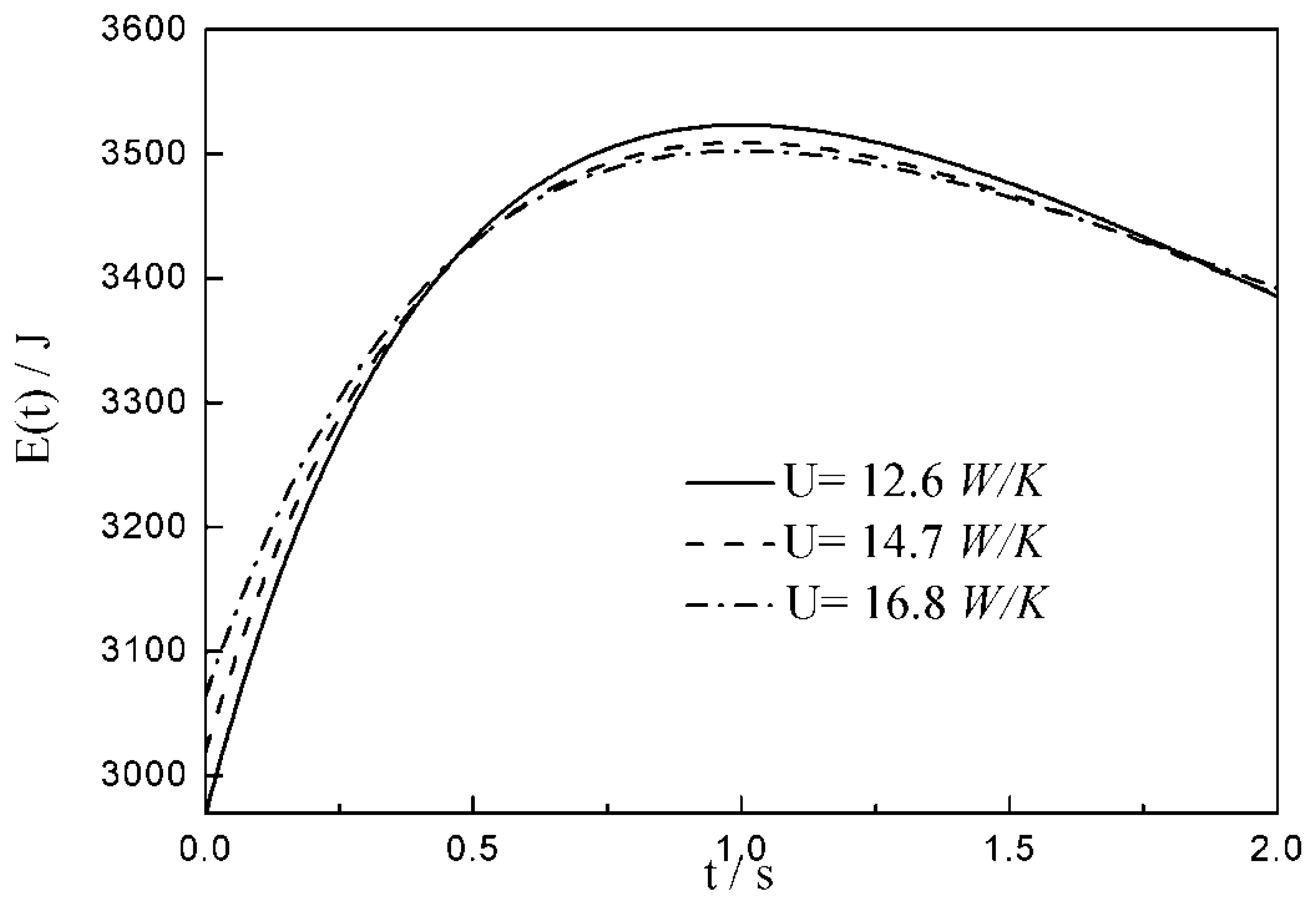
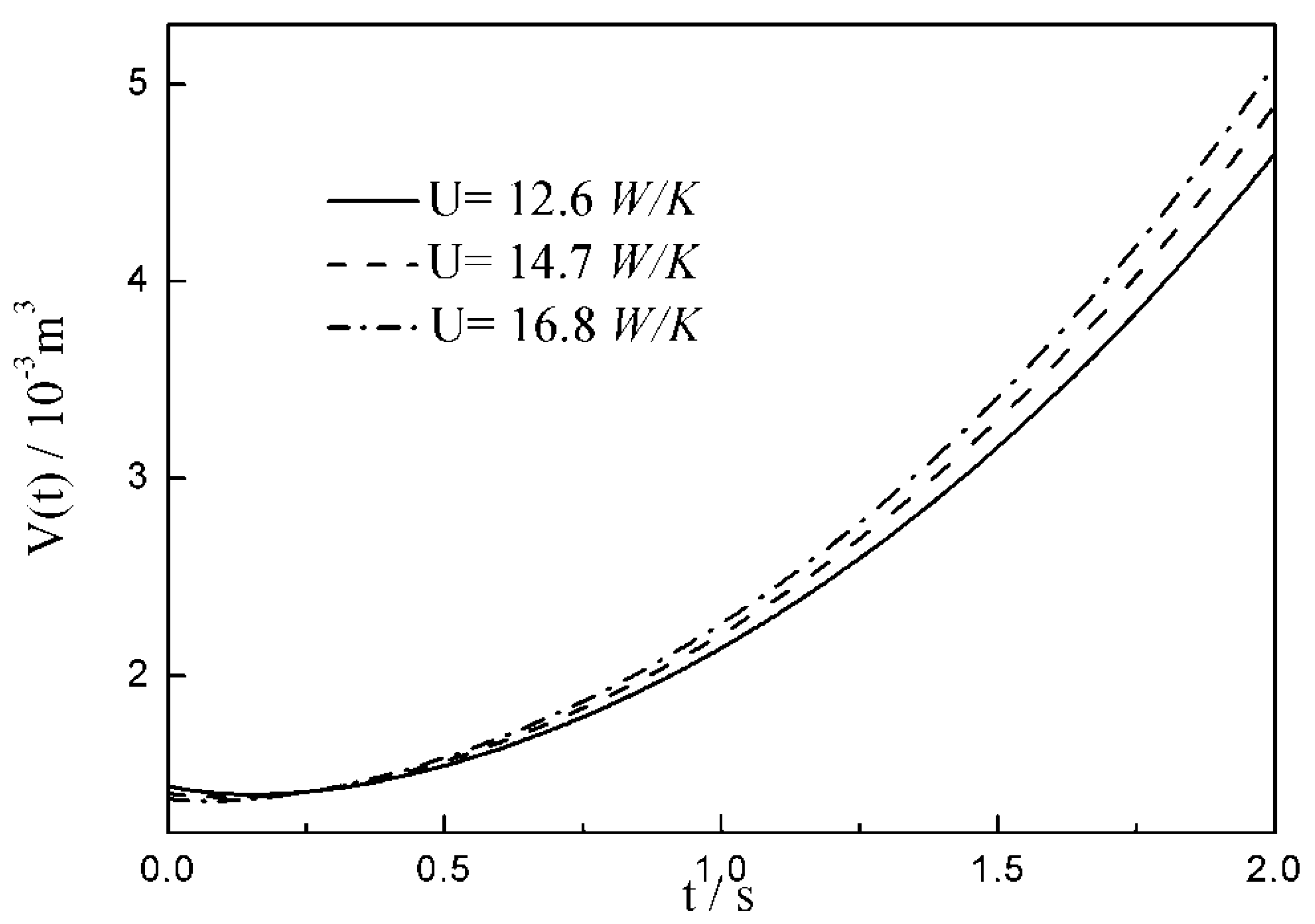
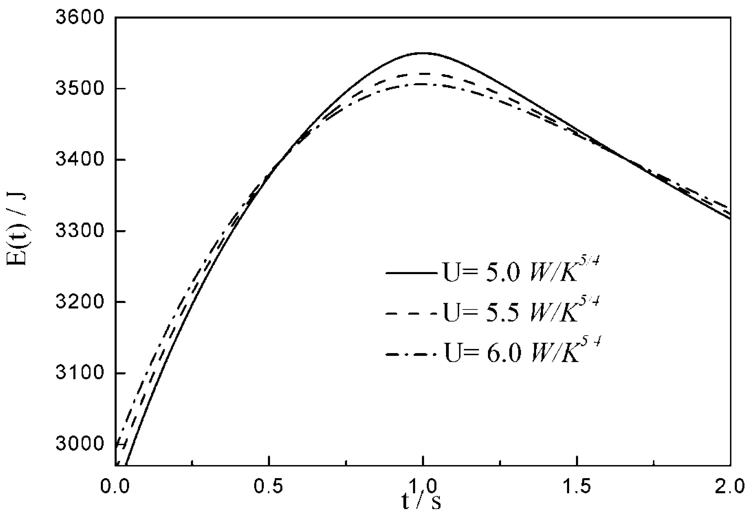
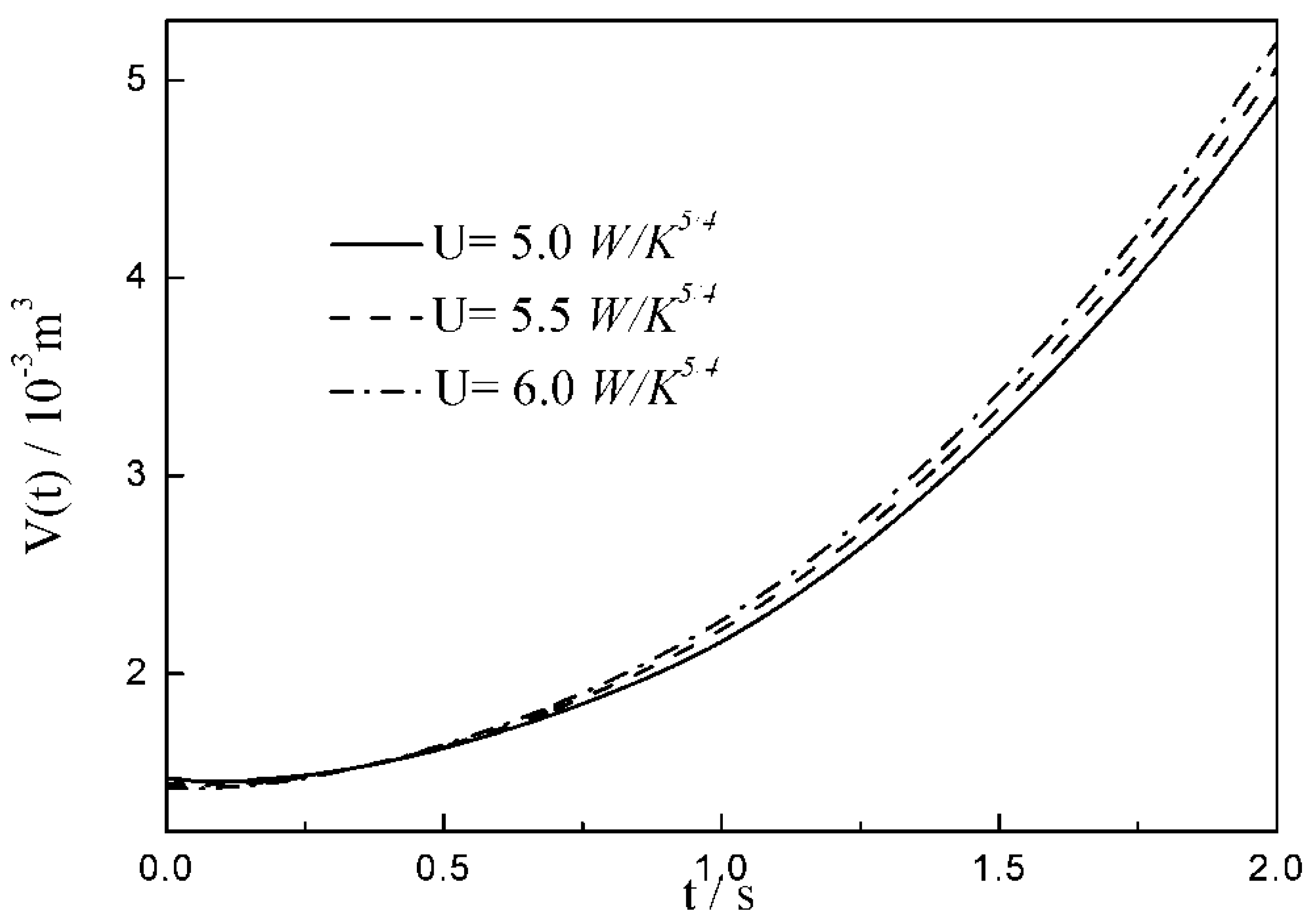
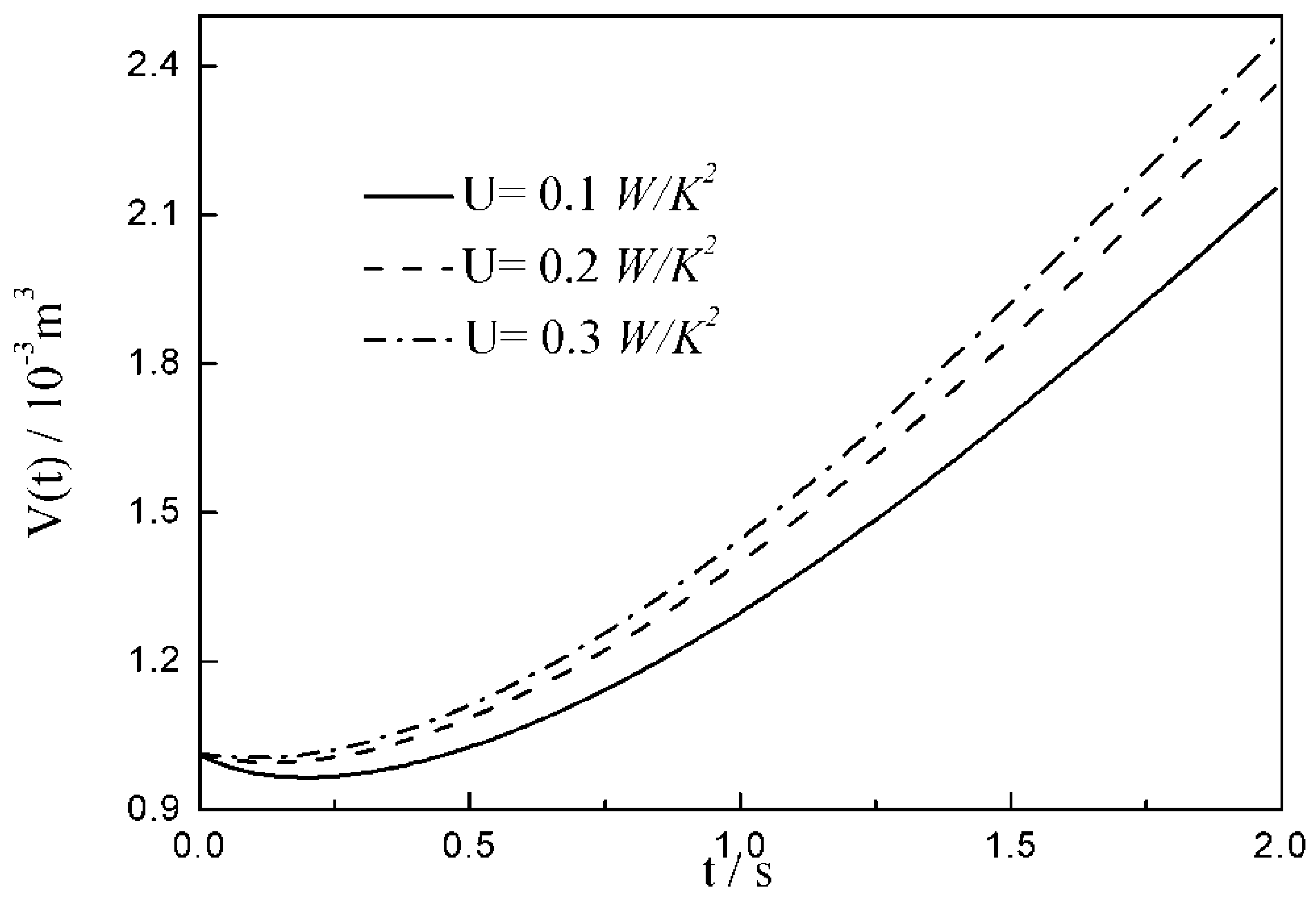
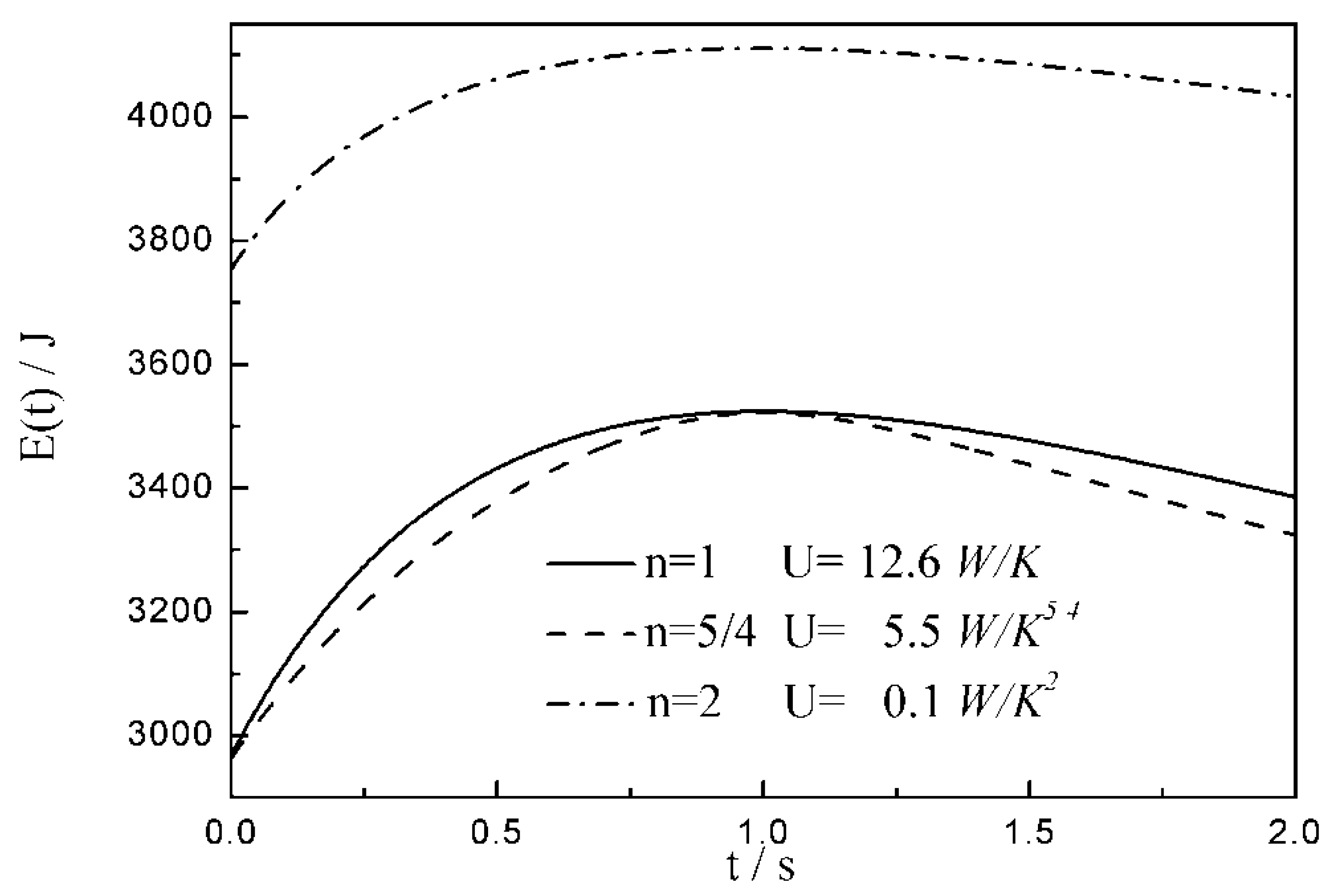
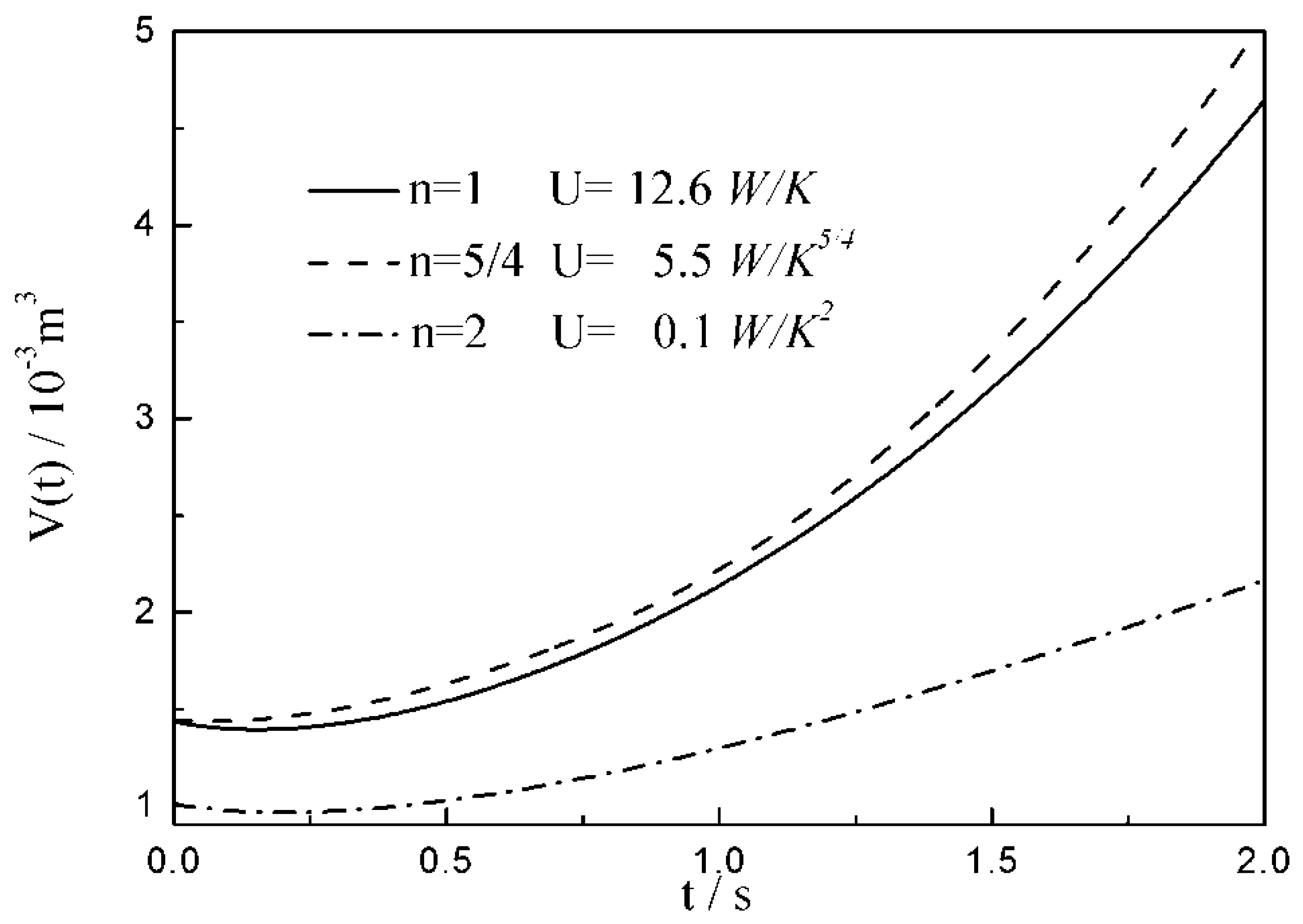
The relationships between the $E$ and time are similar under the conditions of three special heat transfer laws; namely, the $E$ increases to the peak before decreasing with the increase in time, and there is a maximum $E$. For all of three special heat transfer laws, the working fluid is compressed slightly in the initial $E-L$ arc, and then monotonically expands until the end of expansion process. with the augmentation of the $U$, $V\left(t_m\right)/$$V^{\prime }\left(0\right)$ of working fluid during the $E-L$ arc increases.

(2)

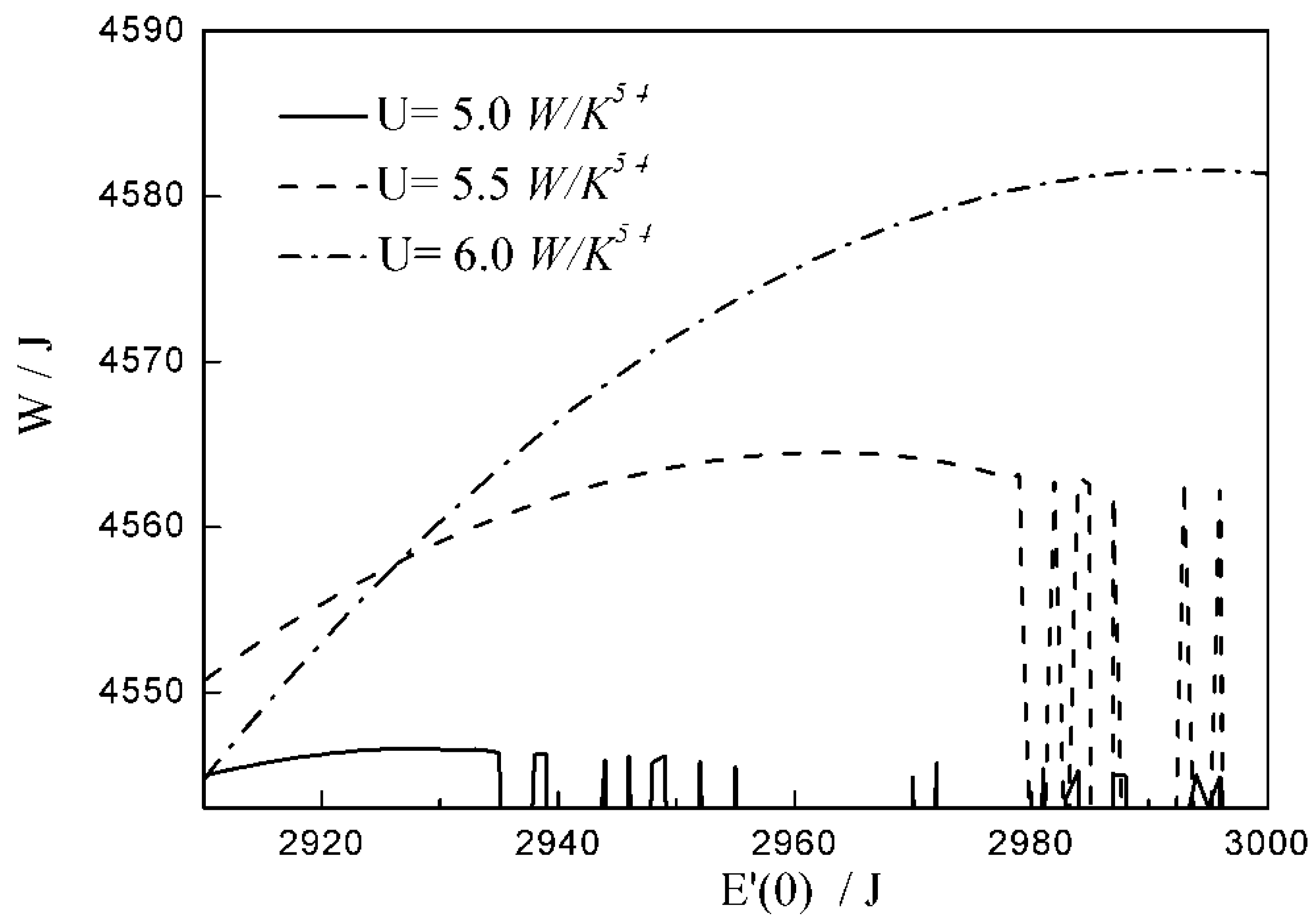
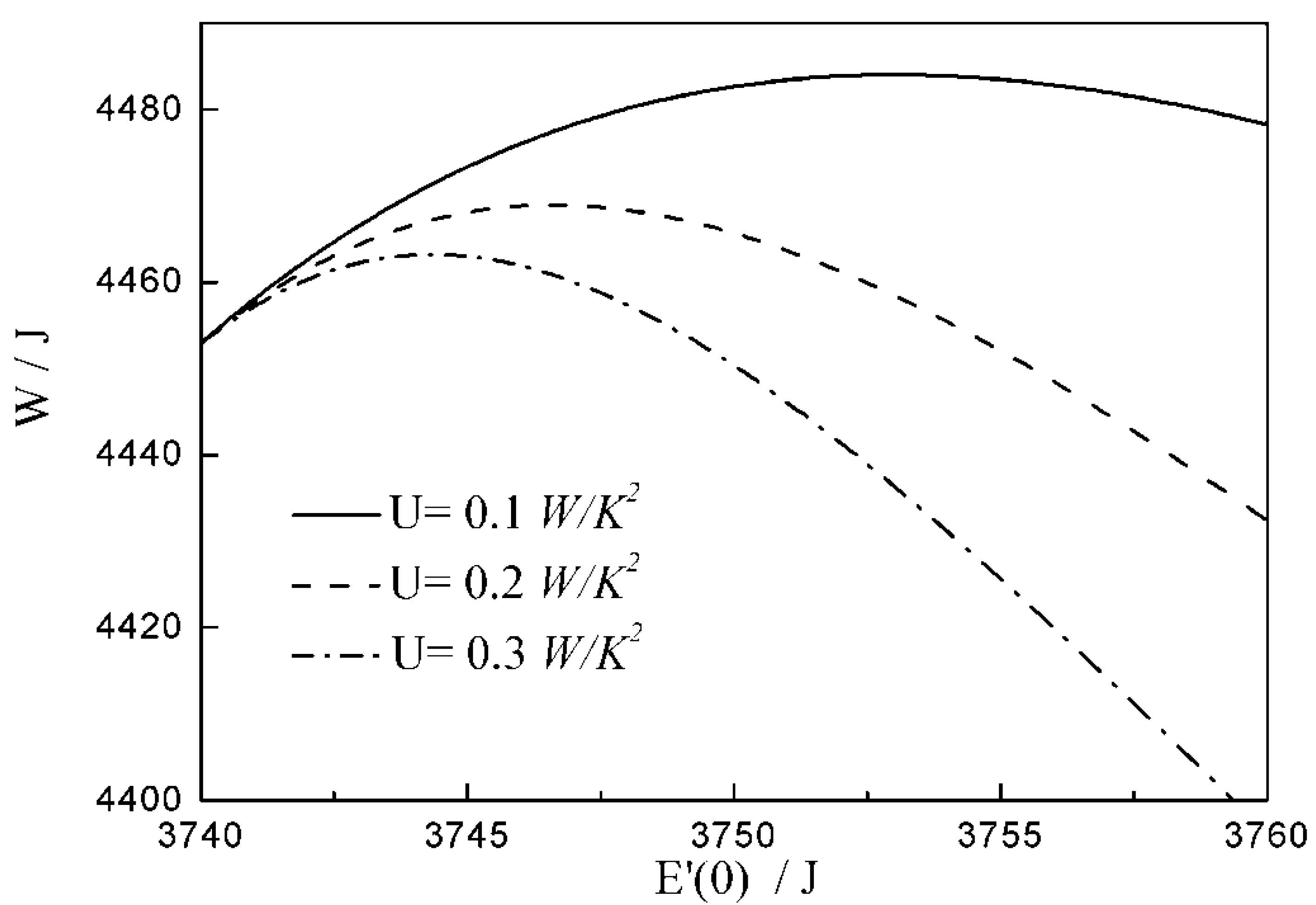
There are differences among the optimal configurations with three different heat transfer laws. In the cases of $n=1$ and $n=5/4$, the temperature at which the whole $E-L$ arc occurs should be below the external heat bath temperature, namely less than $T_{ex}=300 \mathrm{K}$; with the augmentation of $U$, the $V^{\prime }\left(0\right)$ decreases, and the $E^{\prime }\left(0\right)$, maximum work output and ${\eta }_W$ increase. While for $n=2$, the temperature at which the whole $E-L$ arc occurs should be above the external heat bath temperature, namely more than $T_{ex}=300 \mathrm{K}$. This indicates that the working fluid does not absorb heat from the external heat bath, but releases heat to the external heat bath during the whole $E-L$ arc. With the augmentation of $U$, the $V^{\prime }\left(0\right)$ increases, and the $E^{\prime }\left(0\right)$, maximum work output and ${\eta }_W$ decrease. The results obtained with $n=2$ are not only different from those with $n=1$ and $n=5/4$, but also from those with square $\left(T^2-T_{ex}^2\right)$, cubic $\left(T^3-T_{ex}^3\right)$ and radiative $\left(T^4-T_{ex}^4\right)$ heat transfer laws obtained in the previous studies. Moreover, compared with $n=$ 1 and $n=5/4$, the maximum work output and ${\eta }_W$ with $n=$ 2 are smaller. It can be concluded that the heat transfer law has both quantitative and qualitative influences on the optimal configurations of the expansion process.

(3)

The generalized convective heat transfer law $q\propto {\left(T-T_{ex}^{}\right)}^n$ is introduced into the theoretical model of an ideal gas irreversible expansion process in a piston-type cylinder, so the results obtained are universal and fully reveal the effect of heat transfer laws. The work in this paper can enrich FTT theory.

References

- Andresen, B.; Berry, R.S.; Ondrechen, M.J.; Salamon, P. Thermodynamics for processes in finite time. Acc. Chem. Res. 1984, 17, 266–271. [Google Scholar] [CrossRef]
- Berry, R.S.; Kazakov, V.A.; Sieniutycz, S.; Szwast, Z.; Tsirlin, A.M. Thermodynamic Optimization of Finite Time Processes; Wiley: Chichester, UK, 1999. [Google Scholar]
- Chen, L.G.; Wu, C.; Sun, F.R. Finite time thermodynamic optimization or entropy generation minimization of energy systems. J. Non-Equilib. Thermodyn. 1999, 24, 327–359. [Google Scholar] [CrossRef]
- Hoffmann, K.H.; Burzler, J.; Fischer, A.; Schaller, M.; Schubert, S. Optimal process paths for endoreversible systems. J. Non-Equilib. Thermodyn. 2003, 28, 233–268. [Google Scholar] [CrossRef]
- Chen, L.G.; Sun, F.R. Advances in Finite Time Thermodynamics: Analysis and Optimization; Nova Science Publishers: New York, NY, USA, 2004. [Google Scholar]
- Sieniutycz, S. Thermodynamic Approaches in Engineering Systems; Elsevier: Oxford, UK, 2016. [Google Scholar]
- Feidt, M. Finite Physical Dimensions Optimal Thermodynamics 1. Fundamental; ISTE Press and Elsevier: London, UK, 2017. [Google Scholar]
- Badescu, V. Optimal Control in Thermal Engineering; Springer: New York, NY, USA, 2017. [Google Scholar]
- Chen, L.G.; Xia, S.J. Generalized Thermodynamic Dynamic-Optimization for Irreversible Cycles- Thermodynamic and Chemical Theoretical Cycles; Science Press: Beijing, China, 2018. (In Chinese) [Google Scholar]
- Chen, L.G.; Xia, S.J. Generalized Thermodynamic Dynamic-Optimization for Irreversible Cycles–Engineering Thermodynamic Plants and Generalized Engine Cycles; Science Press: Beijing, China, 2018. (In Chinese) [Google Scholar]
- Chen, L.G.; Xia, S.J. Progresses in generalized thermodynamic dynamic-optimization of irreversible processes. Sci. Sin. Technol. 2019, 49, 981–1022. [Google Scholar] [CrossRef] [Green Version]
- Chen, L.G.; Xia, S.J.; Feng, H.J. Progress in generalized thermodynamic dynamic-optimization of irreversible cycles. Sci. Sin. Technol. 2019, 49, 1223–1267. [Google Scholar] [CrossRef] [Green Version]
- Chen, L.G.; Li, J. Thermodynamic Optimization Theory for Two-Heat-Reservoir Cycles; Science Press: Beijing, China, 2020. [Google Scholar]
- Boikov, S.Y.; Andresen, B.; Akhremenkov, A.A.; Tsirlin, A.M. Evaluation of irreversibility and optimal organization of an integrated multi-stream heat exchange system. J. Non-Equilib. Thermodyn. 2020, 45, 155–171. [Google Scholar] [CrossRef]
- Li, P.L.; Chen, L.G.; Xia, S.J.; Zhang, L. Entropy generation rate minimization for in methanol synthesis via CO2 hydrogenation reactor. Entropy 2019, 21, 174. [Google Scholar] [CrossRef] [Green Version]
- Zhang, L.; Chen, L.G.; Xia, S.J.; Ge, Y.L.; Wang, C.; Feng, H.J. Multi-objective optimization for helium-heated reverse water gas shift reactor by using NSGA-II. Int. J. Heat Mass Transfer 2020, 148, 119025. [Google Scholar] [CrossRef]
- Kingston, D.; Razzitte, A.C. Entropy generation minimization in Dimethyl Ether synthesis: A case study. J. Non-Equilib. Thermodyn. 2018, 43, 111–120. [Google Scholar] [CrossRef]
- Li, P.L.; Chen, L.G.; Xia, S.J.; Zhang, L.; Kong, R.; Ge, Y.L.; Feng, H.J. Entropy generation rate minimization for steam methane reforming reactor heated by molten salt. Energy Rep. 2020, 6, 685–697. [Google Scholar] [CrossRef]
- Marsik, F.; Weigand, B.; Tomas, M.; Tucek, O.; Novotny, P. On the efficiency of electrochemical devices from the perspective of endoreversible thermodynamics. J. Non-Equilib. Thermodyn. 2019, 44, 425–438. [Google Scholar] [CrossRef]
- Roach, T.N.F.; Salamon, P.; Nulton, J.; Andresen, B.; Felts, B.; Haas, A.; Calhoun, S.; Robinett, N.; Rohwer, F. Application of finite-time and control thermodynamics to biological processes at multiple scales. J. Non-Equilib. Thermodyn. 2018, 43, 193–210. [Google Scholar] [CrossRef] [Green Version]
- Barranco-Jimenez, M.A.; Ramos-Gayosso, I.; Rosales, M.A.; Angulo-Brown, F. A proposal of ecologic taxes based on thermoeconomic performance of heat engine models. Energies 2009, 2, 1042–1056. [Google Scholar] [CrossRef]
- Schwalbe, K.; Hoffmann, K.H. Novikov engine with fluctuating heat bath temperature. J. Non-Equilib. Thermodyn. 2018, 43, 141–150. [Google Scholar] [CrossRef]
- Schwalbe, K.; Hoffmann, K.H. Stochastic Novikov engine with Fourier heat transport. J. Non-Equilib. Thermodyn. 2019, 44, 417–424. [Google Scholar] [CrossRef]
- Paéz-Hernández, R.T.; Chimal-Eguía, J.C.; Sánchez-Salas, N.; Ladino-Luna, D. General properties for an Agrawal thermal engine. J. Non-Equilib. Thermodyn. 2018, 43, 131–140. [Google Scholar] [CrossRef]
- Feidt, M.; Costea, M. From finite time to finite physical dimensions thermodynamics: The Carnot engine and Onsager’s relations revisited. J. Non-Equilib. Thermodyn. 2018, 43, 151–162. [Google Scholar] [CrossRef]
- Zaeva, M.A.; Tsirlin, A.M.; Didina, O.V. Finite time thermodynamics: Realizability domain of heat to work converters. J. Non-Equilib. Thermodyn. 2019, 44, 181–191. [Google Scholar] [CrossRef]
- Schwalbe, K.; Hoffmann, K.H. Optimal control of an endoreversible solar power plant. J. Non-Equilib. Thermodyn. 2018, 43, 255–272. [Google Scholar] [CrossRef]
- Wu, Z.X.; Chen, L.G.; Feng, H.J. Thermodynamic optimization for an endoreversible Dual-Miller cycle (DMC) with finite speed of piston. Entropy 2018, 20, 165. [Google Scholar] [CrossRef] [Green Version]
- You, J.; Chen, L.G.; Wu, Z.X.; Sun, F.R. Thermodynamic performance of Dual-Miller cycle (DMC) with polytropic processes based on power output, thermal efficiency and ecological function. Sci. China Technol. Sci. 2018, 61, 453–463. [Google Scholar] [CrossRef]
- Raman, R.; Kumar, N. Performance analysis of Diesel cycle under efficient power density condition with variable specific heat of working fluid. J. Non-Equilib. Thermodyn. 2019, 44, 405–416. [Google Scholar] [CrossRef]
- Abedinnezhad, S.; Ahmadi, M.H.; Pourkiaei, S.M.; Pourfayaz, F.; Mosavi, A.; Feidt, M.; Shamshirband, S. Thermodynamic assessment and multi-objective optimization of performance of irreversible Dual-Miller cycle. Energies 2019, 12, 4000. [Google Scholar] [CrossRef] [Green Version]
- Chen, L.G.; Ge, Y.L.; Liu, C.; Feng, H.J.; Lorenzini, G. Performance of universal reciprocating heat-engine cycle with variable specific heats ratio of working fluid. Entropy 2020, 22, 397. [Google Scholar] [CrossRef] [Green Version]
- Chen, L.G.; Meng, F.K.; Sun, F.R. Thermodynamic analyses and optimizations for thermoelectric devices: The state of the arts. Sci. China: Technol. Sci. 2016, 59, 442–455. [Google Scholar] [CrossRef]
- Feng, Y.L.; Chen, L.G.; Meng, F.K.; Sun, F.R. Influences of external heat transfer and Thomson effect on performance of TEG-TEC combined thermoelectric device. Sci. China: Technol. Sci. 2018, 61, 1600–1610. [Google Scholar] [CrossRef]
- Li, G.; Wang, Z.C.; Wang, F.; Wang, X.Z.; Li, S.B.; Xue, M.S. Experimental and numerical study on the effect of interfacial heat transfer on performance of thermoelectric generators. Energies 2019, 12, 3797. [Google Scholar] [CrossRef] [Green Version]
- Chen, L.G.; Meng, F.K.; Ge, Y.L.; Feng, H.J.; Xia, S.J. Performance optimization of a class of combined thermoelectric heating devices. Sci. China: Technol. Sci. 2020, 63. [Google Scholar] [CrossRef]
- Dumitrascu, G.; Feidt, M.; Popescu, A.; Grigorean, S. Endoreversible trigeneration cycle design based on finite physical dimensions thermodynamics. Energies 2019, 12, 3165. [Google Scholar]
- Feng, H.J.; Tao, G.S.; Tang, C.Q.; Ge, Y.L.; Chen, L.G.; Xia, S.J. Exergoeconomic performance optimization for a regenerative gas turbine closed-cycle heat and power cogeneration plant. Energy Rep. 2019, 5, 1525–1531. [Google Scholar] [CrossRef]
- Chen, L.G.; Yang, B.; Feng, H.J.; Ge, Y.L.; Xia, S.J. Performance optimization of an open simple-cycle gas turbine combined cooling, heating and power plant driven by basic oxygen furnace gas in China’s steelmaking plants. Energy 2020, 203, 117791. [Google Scholar] [CrossRef]
- Fontaine, K.; Yasunaga, T.; Ikegami, Y. OTEC maximum net power output using Carnot cycle and application to simplify heat exchanger selection. Entropy 2019, 21, 1143. [Google Scholar] [CrossRef] [Green Version]
- Wu, Z.X.; Feng, H.J.; Chen, L.G.; Tang, W.; Shi, J.Z.; Ge, Y.L. Constructal thermodynamic optimization for ocean thermal energy conversion system with dual-pressure organic Rankine cycle. Energy Convers. Manag. 2020, 210, 112727. [Google Scholar] [CrossRef]
- Yasunaga, T.; Ikegami, Y. Finite-time thermodynamic model for evaluating heat engines in ocean thermal energy conversion. Entropy 2020, 22, 211. [Google Scholar] [CrossRef] [Green Version]
- Feng, H.J.; Qin, W.X.; Chen, L.G.; Cai, C.G.; Ge, Y.L.; Xia, S.J. Power output, thermal efficiency and exergy-based ecological performance optimizations of an irreversible KCS-34 coupled to variable temperature heat reservoirs. Energy Convers. Manag. 2020, 205, 112424. [Google Scholar] [CrossRef]
- Chen, W.J.; Feng, H.J.; Chen, L.G.; Xia, S.J. Optimal performance characteristics of subcritical simple irreversible organic Rankine cycle. J. Therm. Sci. 2018, 27, 555–562. [Google Scholar] [CrossRef]
- Wang, S.; Zhang, W.; Feng, Y.Q.; Wang, X.; Wang, Q.; Liu, Y.Z.; Wang, Y.; Yao, L. Entropy, entransy and exergy analysis of a dual-loop organic Rankine cycle (DORC) using mixture working fluids for engine waste heat recovery. Energies 2020, 13, 1301. [Google Scholar] [CrossRef] [Green Version]
- Feng, H.J.; Chen, W.J.; Chen, L.G.; Tang, W. Power and efficiency optimizations of an irreversible regenerative organic Rankine cycle. Energy Convers. Manag. 2020, 220, 113079. [Google Scholar] [CrossRef]
- Tang, C.Q.; Feng, H.J.; Chen, L.G.; Wang, W.H. Power density analysis and multi-objective optimization for a modified endoreversible simple closed Brayton cycle with one isothermal heating process. Energy Rep. 2020, 6. in pres. [Google Scholar]
- Chen, L.G.; Feng, H.J.; Ge, Y.L. Power and efficiency optimization for open combined regenerative Brayton and inverse Brayton cycles with regeneration before the inverse cycle. Entropy 2020, 22, 677. [Google Scholar] [CrossRef]
- Tang, C.Q.; Chen, L.G.; Feng, H.J.; Wang, W.H.; Ge, Y.L. Power optimization of a closed binary Brayton cycle with isothermal heating processes and coupled to variable-temperature reservoirs. Energies 2020, 13, 3212. [Google Scholar]
- Zhu, F.L.; Chen, L.G.; Wang, W.H. Thermodynamic analysis of an irreversible Maisotsenko reciprocating Brayton cycle. Entropy 2018, 20, 167. [Google Scholar] [CrossRef] [Green Version]
- Chen, L.G.; Shen, J.F.; Ge, Y.L.; Wu, Z.X.; Wang, W.H.; Zhu, F.L.; Feng, H.J. Power and efficiency optimization of open Maisotsenko-Brayton cycle and performance comparison with traditional open regenerated Brayton cycle. Energy Convers. Manag. 2020, 217, 113001. [Google Scholar] [CrossRef]
- Ding, Z.M.; Ge, Y.L.; Chen, L.G.; Feng, H.J.; Xia, S.J. Optimal performance regions of Feynman’s ratchet engine with different optimization criteria. J. Non-Equilib. Thermodyn. 2020, 45, 191–207. [Google Scholar] [CrossRef]
- Ding, Z.M.; Chen, L.G.; Ge, Y.L.; Xie, Z.H. Optimal performance regions of an irreversible energy selective electron heat engine with double resonance. Sci. China: Technol. Sci. 2019, 62, 397–405. [Google Scholar] [CrossRef]
- Meng, Z.W.; Chen, L.G.; Wu, F. Optimal power and efficiency of multi-stage endoreversible quantum Carnot heat engine with harmonic oscillators at the classical limit. Entropy 2020, 22, 457. [Google Scholar] [CrossRef] [Green Version]
- Rubin, M.H. Optimal configuration of a class of irreversible heat engines. Phys. Rev. A 1979, 19, 1272–1287. [Google Scholar] [CrossRef]
- Rubin, M.H. Optimal configuration of an irreversible heat engine with fixed compression ratio. Phys. Rev. A 1980, 22, 1741–1752. [Google Scholar] [CrossRef]
- Ondrechen, M.J.; Rubin, M.H.; Band, Y.B. The generalized Carnot cycles: A working fluid operating in finite-time between finite heat sources and sinks. J. Chem. Phys. 1983, 78, 4721–4727. [Google Scholar] [CrossRef]
- Chen, L.G.; Zhou, S.B.; Sun, F.R.; Wu, C. Optimal configuration and performance of heat engines with heat leak and finite heat capacity. Open Syst. Inf. Dyn. 2002, 9, 85–96. [Google Scholar] [CrossRef]
- Mozurkewich, M.; Berry, R.S. Finite-time thermodynamics: Engine performance improved by optimized piston motion. Proc. Natl. Acad. Sci. USA 1981, 78, 1986–1988. [Google Scholar] [CrossRef] [PubMed] [Green Version]
- Mozurkewich, M.; Berry, R.S. Optimal paths for thermodynamic systems. The ideal Otto cycle. J. Appl. Phys. 1982, 53, 34–42. [Google Scholar] [CrossRef]
- Hoffmann, K.H.; Watowich, S.J.; Berry, R.S. Optimal paths for thermodynamic systems. The ideal Diesel cycle. J. Appl. Phys. 1985, 58, 2125–2134. [Google Scholar] [CrossRef]
- Blaudeck, P.; Hoffmann, K.H. Optimization of the power output for the compression and power stroke of the Diesel engine. In Proceedings of the International Conference ECOS’95, Istanbul, Turkey, 11–14 July 1995; Volume 2, p. 754. [Google Scholar]
- Watowich, S.J.; Hoffmann, K.H.; Berry, R.S. Intrinsically irreversible light-driven engine. J. Appl. Phys. 1985, 58, 2893–2901. [Google Scholar] [CrossRef]
- Watowich, S.J.; Hoffmann, K.H.; Berry, R.S. Optimal path for a bimolecular, light –driven engine. IL Nuovo Cimento B 1989, 104B, 131–147. [Google Scholar] [CrossRef]
- Teh, K.Y.; Miller, S.L.; Edwards, C.F. Thermodynamic requirements for maximum internal combustion engine cycle efficiency Part 1: Optimal combustion strategy. Int. J. Engine Res. 2008, 9, 449–465. [Google Scholar] [CrossRef]
- Teh, K.Y.; Miller, S.L.; Edwards, C.F. Thermodynamic requirements for maximum internal combustion engine cycle efficiency Part 2: Work extraction and reactant preparation strategies. Int. J. Engine Res. 2008, 9, 467–481. [Google Scholar] [CrossRef]
- Bi, Y.H.; Guo, T.; Zhang, L.; Chen, L.G.; Sun, F.R. Entropy generation minimization for charging and discharging processes in a gas hydrate cool storage system. Appl. Energy 2010, 87, 1149–1157. [Google Scholar] [CrossRef]
- Band, Y.B.; Kafri, O.; Salamon, P. Maximum work production from a heated gas in a cylinder with piston. Chem. Phys. Lett. 1980, 72, 127–130. [Google Scholar] [CrossRef]
- Band, Y.B.; Kafri, O.; Salamon, P. Finite time thermodynamics: Optimal expansion of a heated working fluid. J. Appl. Phys. 1982, 53, 8–28. [Google Scholar] [CrossRef]
- Band, Y.B.; Kafri, O.; Salamon, P. Optimization of a model external combustion engine. J. Appl. Phys. 1982, 53, 29–33. [Google Scholar] [CrossRef]
- Aizenbud, B.M.; Band, Y.B. Power considerations in the operation of a piston fitted inside a cylinder containing a dynamically heated working fluid. J. Appl. Phys. 1981, 52, 3742–3744. [Google Scholar] [CrossRef]
- Salamon, P.; Band, Y.B.; Kafri, O. Maximum power from a cycling working fluid. J. Appl. Phys. 1982, 53, 197–202. [Google Scholar] [CrossRef]
- Aizenbud, B.M.; Band, Y.B.; Kafri, O. Optimization of a model internal combustion engine. J. Appl. Phys. 1982, 53, 1277–1282. [Google Scholar] [CrossRef]
- Song, H.J.; Chen, L.G.; Li, J.; Sun, F.R.; Wu, C. Optimal configuration of a class of endoreversible heat engines with linear phenomenological heat transfer law []. J. Appl. Phys. 2006, 100, 124907. [Google Scholar] [CrossRef]
- Song, H.J.; Chen, L.G.; Sun, F.R. Endoreversible heat engines for maximum power output with fixed duration and radiative heat-transfer law. Appl. Energy 2007, 84, 374–388. [Google Scholar] [CrossRef]
- Song, H.J.; Chen, L.G.; Sun, F.R.; Wang, S.B. Configuration of heat engines for maximum power output with fixed compression ratio and generalized radiative heat transfer law. J. Non-Equilib. Thermodyn. 2008, 33, 275–295. [Google Scholar] [CrossRef]
- Chen, L.G.; Song, H.J.; Sun, F.R.; Wang, S.B. Optimal configuration of heat engines for maximum efficiency with generalized radiative heat transfer law. Rev. Mexi. Fis. 2009, 55, 55–67. [Google Scholar]
- Chen, L.G.; Song, H.J.; Sun, F.R.; Wu, C. Optimal configuration of heat engines for maximum power with generalized radiative heat transfer law. Int. J. Ambient Energy 2009, 30, 137–160. [Google Scholar] [CrossRef]
- Chen, L.G.; Song, H.B.; Sun, F.R. Endoreversible radiative heat engines for maximum efficiency. Appl. Math. Modell. 2010, 34, 1710–1720. [Google Scholar] [CrossRef]
- Yan, Z.J.; Chen, J.C. Optimal performance of a generalized Carnot cycle for another linear heat transfer law. J. Chem. Phys. 1990, 92, 1994–1998. [Google Scholar] [CrossRef]
- Xiong, G.; Chen, J.C.; Yan, Z.J. The effect of heat transfer law on the performance of a generalized Carnot cycle. J. Xiamen Univ. 1989, 28, 489–494. (In Chinese) [Google Scholar]
- Chen, L.G.; Zhu, X.; Sun, F.R.; Wu, C. Optimal configurations and performance for a generalized Carnot cycle assuming the heat transfer law . Appl. Energy 2004, 78, 305–313. [Google Scholar] [CrossRef]
- Li, J.; Chen, L.G.; Sun, F.R. Optimal configuration for a finite high-temperature source heat engine cycle with complex heat transfer law. Sci. China Ser. G. 2009, 52, 587–592. [Google Scholar] [CrossRef]
- Burzler, M.J.; Hoffmann, K.H. Optimal piston paths for Diesel engines. In Thermodynamics of Energy Conversion and Transport; Sienuitycz, S., de Vos, A., Eds.; Springer: New York, NY, USA, 2000; Chapter 7. [Google Scholar]
- Burzler, J.M. Performance Optima for Endoreversible Systems. Ph.D. Thesis, University of Chemnitz, Chemnitz, Germany, 2002. [Google Scholar]
- Xia, S.J.; Chen, L.G.; Sun, F.R. Optimal path of piston motion for Otto cycle with linear phenomenological heat transfer law. Sci. China Ser. G 2009, 52, 708–719. [Google Scholar] [CrossRef]
- Ge, Y.L.; Chen, L.G.; Sun, F.R. Optimal paths of piston motion of irreversible Otto cycle heat engines for minimum entropy generation. Sci. China, Phys. Mech. Astron. 2010, 40, 1115–1129. [Google Scholar]
- Ma, K.; Chen, L.G.; Sun, F.R. Optimal paths for a light-driven engine with linear phenomenological heat transfer law. Sci. China, Chem. 2010, 53, 917–926. [Google Scholar] [CrossRef]
- Chen, L.G.; Sun, F.R.; Wu, C. Optimal expansion of a heated working fluid with phenomenological heat transfer. Energy Convers. Mgmt. 1998, 39, 149–156. [Google Scholar] [CrossRef]
- Song, H.J.; Chen, L.G.; Sun, F.R. Optimal expansion of a heated working fluid for maximum work output with generalized radiative heat transfer law. J. Appl. Phys. 2007, 102, 094901. [Google Scholar] [CrossRef]
- Chen, L.G.; Song, H.J.; Sun, F.R.; Wu, C. Optimal expansion of a heated working fluid with convective- radiative heat transfer law. Int. J. Ambient Energy 2010, 31, 81–90. [Google Scholar] [CrossRef]
- Chen, L.G.; Ma, K.; Ge, Y.L.; Feng, H.J. Re-optimization of expansion work of a heated working fluid with generalized radiative heat transfer law. Entropy 2020, 22. in press. [Google Scholar]
- Song, H.J.; Chen, L.G.; Sun, F.R. Optimization of a model external combustion engine with linear phenomenological heat transfer law. J. Energy Inst. 2009, 82, 180–183. [Google Scholar] [CrossRef]
- Chen, L.G.; Song, H.J.; Sun, F.R.; Wu, C. Optimization of a model internal combustion engine with linear phenomenological heat transfer law. Int. J. Ambient Energy 2010, 31, 13–22. [Google Scholar] [CrossRef]
- Gutowicz-Krusin, D.; Procaccia, J.; Ross, J. On the efficiency of rate processes: Power and efficiency of heat engines. J. Chem. Phys. 1978, 69, 3898–3906. [Google Scholar] [CrossRef]
- Angulo-Brown, F.; Paez-Hernandez, R. Endoreversible thermal cycle with a nonlinear heat transfer law. J. Appl. Phys. 1993, 74, 2216–2219. [Google Scholar] [CrossRef]
- Chen, L.G.; Sun, F.R.; Wu, C. Influence of heat transfer law on the performance of a Carnot engine. Appl. Thermal Eng. 1997, 17, 277–282. [Google Scholar] [CrossRef]
- Zhou, S.B.; Chen, L.G.; Sun, F.R. Optimal performance of a generalized irreversible Carnot engine. Appl. Energy 2005, 81, 376–387. [Google Scholar] [CrossRef]
- Huleihil, M.; Andresen, B. Convective heat transfer law for an endoreversible engine. J. Appl. Phys. 2006, 100, 014911. [Google Scholar] [CrossRef] [Green Version]
- O’Sullivan, C.T. Newton’s law of cooling-A critical assessment. Am. J. Phys. 1990, 58, 956–960. [Google Scholar] [CrossRef]