Enabling Methodologies for Predictive Power System Resilience Analysis in the Presence of Extreme Wind Gusts


Department of Engineering (DING), University of Sannio, 82100 Benevento, Italy
*
Author to whom correspondence should be addressed.
Energies 2020, 13(13), 3501; https://doi.org/10.3390/en13133501
Submission received: 23 May 2020
/
Revised: 25 June 2020
/
Accepted: 2 July 2020
/
Published: 7 July 2020
(This article belongs to the Special Issue Data Mining in Smart Grids)
Abstract
:Modern power system operation should comply with strictly reliability and security constraints, which aim at guarantee the correct system operation also in the presence of severe internal and external disturbances. Amongst the possible phenomena perturbing correct system operation, the predictive assessment of the impacts induced by extreme weather events has been considered as one of the most critical issues to address, since they can induce multiple, and large-scale system contingencies. In this context, the development of new computing paradigms for resilience analysis has been recognized as a very promising research direction. To address this issue, this paper proposes two methodologies, which are based on Time Varying Markov Chain and Dynamic Bayesian Network, for assessing the system resilience against extreme wind gusts. The main difference between the proposed methodologies and the traditional solution techniques is the improved capability in modelling the occurrence of multiple component faults and repairing, which cannot be neglected in the presence of extreme events, as experienced worldwide by several Transmission System Operators. Several cases studies and benchmark comparisons are presented and discussed in order to demonstrate the effectiveness of the proposed methods in the task of assessing the power system resilience in realistic operation scenarios.
1. Introduction
The modern electric grids operation policies are based on rigorous reliability and recovery principles, which have been defined in order to allow power systems to operate safely against multiple severe contingencies, providing high quality of electricity supply [1]. In the last decades, due to climate change and environmental temperature increase, extreme weather events are becoming more and more common even in non-tropical regions [2]. Electric networks are particularly vulnerable to these events, which can induce multiple power equipment damages, especially in overhead lines and substations. In this context, the deployment of traditional reliability and restoration-based methodologies could fail in assessing the impacts of these extreme events on power system operation, due to their inability in effectively modelling low-probable but possible fault scenario [3]. To address this complex problem, new computing paradigms based on resilience analysis have been proposed in the literature for reducing the grid vulnerability against severe disturbances, and improving the corresponding restoration strategies [4,5,6,7,8,9,10].
Although there is not an universal definition of system resilience, it can be roughly considered as the ability of a system to anticipate and absorb a High Impact Low Probability (HILP) event and regain its normal operating status as quickly as possible [11]. More specifically, according to the UK Energy Research Center [12] the resilience of an electric power system is: “the capacity of an energy system to tolerate disturbance and to continue to deliver affordable energy services to consumers. A resilient energy system can speedily recover from shocks and can provide alternative means of satisfying energy service needs in the event of changed external circumstances”.
This definition outlines the need for defining proper indexes for quantifying the system resilience, in order to assess the effectiveness of mitigation strategies reacting to multiple disruptive events. These strategies can be deployed at both planning and operation stage by (i) improving the infrastructural capacity of the power components to withstand extreme stresses; and (ii) reducing the restoration times, by preemptively identifying proper control actions aimed at mitigating the effects of multiple contingencies, and reducing the restoration times. To this aim, the deployment of the traditional N-1 reliability principle does not allow to obtain a reliable analysis in the presence of severe contingencies induced by multiple HILP events. Anyway, evolving from the N-1 to N-k criterion is not a trivial issue to address due to the prohibitive computational costs of considering a wider, and more severe, set of multiple and correlated contingencies. Hence, the employment of probabilistic risk-based approach, which are characterized by relaxed constraints, may be a good trade-off point.
In this context, the development of risk-based methodologies for power system resilience assessment represents a relevant issue to address in order to estimate the actual system vulnerability against HILP events, the expected impacts on system operation, and the effectiveness of the potential countermeasures.
The possible strategies that can be deployed for solving this issue can be classified into two main groups: ex-post and ex-ante analyses. The first class of methods try to infer from operation data related to past outages, the system resilience against each perturbation events over large operation periods. Besides, these methods can contribute to qualitatively identify in which domains the system operator can intervene for increasing the system resilience, e.g., component design, system restoration, network planning and operation.
A different, and more interesting, prospective is offered by ex-ante methods, which aim at identifying preemptive actions, satisfying fixed system resilience requirements. This is a strategic feature, since power systems operators are compelled to reliably predicting the occurrence and the impacts of “extreme events”, in order to be able to manage and mitigate their effects on system operation. Moreover, ex-ante methods allow effectively modelling the impacts of various source of uncertainties on system resilience analysis, as far as load forecasts errors, renewable power generators randomness and uncertain power transactions are concerned.
Nowadays, most of the ex-ante methodologies for resilience analysis proposed in the literature are based on Monte Carlo simulations (MCS), which aim at generating synthetic time series representing the system behavior under different weather conditions [4,5,6,7,10], and probabilistic techniques based on the minimal path algorithm, which is applied to identify optimal restoration paths based on the definition of “resilience factors” associated at each component [13,14,15,16,17]. Although these methods allow obtaining valuable information about the potential impacts of severe perturbations on system operation, they may fail to model the complex correlations between multiple disruptive events and components fault rates. These limitations mainly derive by the simplified assumptions that need to be assumed in order to make the problem tractable.
To address this complex problem, the deployment of Dynamic Bayesian Networks (DBNs) represents a very promising research direction. These methods allow predicting the impacts of multiple HILP and cascade events on both system operation and restoration, by considering a plurality of possible events and consequences [8,9]. However, the deployment of these DBNs in power system resilience analysis is still at its infancy, and requires further research efforts aimed at developing computational methods for deep simulations, which should be able to assess and compare the correlations of the physical parameters affected by the HILP events with the components fault models, and the corresponding propagation scenarios, from the starting event up to black out and recovery.
Moreover, the computational burden of these methods could be a limiting factor for on-line predictive resilience analysis, which requires problem solutions in very short time-frames, especially if these solutions should be used as input for further computational processes, such as loss of load estimation, and on-line power system contingency analysis.
Finally, new methods aimed at lowering the information granularity of the components fault models in function of their spatial location, and the expected magnitude of the perturbation events are necessary in order to improve the effectiveness of the resiliency analysis, especially for power systems distributed along large geographical area.
On the basis of this literature analysis, it can be argue that the research for new methods aimed at solving the accuracy versus complexity dichotomy in power system resiliency assessment represents a relevant issue to address.
In trying and solving this issue, this paper analyzes the potential role of adaptive probabilistic models for predictive resiliency analysis in the presence of extreme wind gusts, which have been recognized as one of the most critical weather phenomena affecting many European power systems. The adoption of these models allows adapting the component fault parameters in function of the forecast spatial/temporal wind speed evolution, as far as to dynamically estimate the impacts of multiple faults on power system operation, the corresponding worst-case scenario and its occurrence probability. The main innovations of these methods compared to other traditional techniques can be summarized as follows:
- Differently from the regional approach proposed in [4], a more detailed characterization of wind spatial profiles, which have been acquired by pervasive sensor devices deployed over the lines, has been performed in order to assess their impact on the system components. This leads to resiliency analysis characterized by higher spatial resolution. In particular, the spatial resolution increment in large network disruption analysis is crucial to face adequately with HILP events as described by [18].
- The analyzed power system is modelled without assuming any simplified network equivalent;
- Differently from the DBN-based approach proposed in [9], the parameters of the components fault model are correlated to the weather effects;
- Differently from the approach proposed in [8], the cascade effects induced by multiple components failure are modelled by dynamically adapting the power system topology, which allows lowering the complexity of the assessment procedure.
Several cases studies and benchmark comparisons are presented and discussed in order to demonstrate the effectiveness of the proposed methods in the task of assessing the power system resilience in realistic operation scenario. For each considered case study, a comprehensive scalability analysis is performed in order to assess the computational burden of the proposed methods in function of the system complexity.
2. Mathematical Preliminaries
Predicting the impacts of disruptive events on system operation is a strategic tool for improving the power systems security, since it allows identifying preemptive actions aimed at mitigating the effects of multiple contingencies induced by these severe events [19]. This computing process, which is usually referred as predictive resilience analysis, requires the solution of a set of probabilistic models aimed at (i) characterizing how the disruptive events affect the components failure parameters, (ii) predicting the corresponding components failures, and (iii) assessing their impacts on power system operation. To this aim, modelling techniques based on Markov Process and Bayesian Network represent the most promising enabling methodologies.
2.1. Markov Chain
A Markov Chain is a memory-less discrete stochastic process, satisfying the so called “Markov property”:
where X is a generic discrete random variable, which assumes a finite number of d possible occurrences (called “state”) . Equation (1) states that the evolution of the system depends only on the present state and not on the past.
Furthermore, if the following equation holds on the process is called “homogeneous”:
The latter assures the process being time-invariant, which means that the transition probability matrix has constant parameters over the time. The transition probability matrix is a square matrix of order d:
whose elements represent the conditional probabilities to be in the state j at the time instant t+1 starting from the state i. One of the main properties of this matrix is that the elements of each row have to guarantee that their sum is equal to 1. Hence, once known the state probability vector at time instant t, the corresponding probabilities at the next step can be computed as it follows:
The state probability vector at the initial time step is a vector with only one element equal to 1. In case the parameters of change over the time the Markov Chain is called “time-variant” and the transition matrix has defined as .
2.2. Bayesian Networks
Bayesian Network (BN) is Directed Acyclic Graph (DAG) that allows representing all the casual relationship among a set of correlated variables. The structure of a Bayesian network is based on two main components:
Description 1.
Nodes: represent a set of variables. Every node has a conditional probability distribution represented through Conditional Probability Table (CPT). Arcs: represent the probabilistic dependencies between the variables. A node is called “parent” of a “child” if there is a direct arc connecting the first to the second.
Each node is characterized by a conditional probability distribution modeled through the Conditional Probability Table (CPT). For each variable , with n parent nodes, , the CPT is indicated as and contains all the probability associated to any possible combination between the states of and all its parents.
By using the chain rule, the joint probability distribution of all the BN nodes can be computed as follows:
3. Proposed Methodology
The aim of this paper is to propose a computationally effective method for assessing the impacts of severe wind gusts on power system operation by deep simulations of probabilistic models. The final goal is to assess the system reaction to the loss of multiple critical network components, whose failure model parameters are adapted in function of predicted time/spatial wind speed profiles. The latter greatly affect the components fault rate, especially in the presence of extremely high wind speeds, which may damage the overhead line conductors, causing multiple and severe faults, as recently experienced in several European power systems [20]. These severe weather phenomena could interest large geographical area, threatening the correct operation of a large number of power components. Consequently, the number of fault scenarios that should be analyzed may exponentially increase, causing an explosion of the problem cardinality, which needs to be properly managed.
To this aim, two different solution methodologies, which are based on time-varying Markov Chains and Dynamic Bayesian Networks, have been developed and compared.
3.1. Improved Time Varying Markov Chains
As introduced in Section 2.1, a MC is entirely defined by its transition matrix, which owns the information about the probability to evolve from a state to another over the time. If the transition rates are time-dependent, the MC is called time-varying, and the transition probability matrix is variable. Thus, the Equation (4) becomes:
where is the probability state vector at time step, whose dimensions are with S number of network states, is the time varying transition probability square matrix of order S, whose parameters are time dependents.
This mathematical tool could play an important role in predictive resilience analysis, since it allows describing the impacts of the time/spatial wind speed profiles on the fault and reparation probability of each network component. To this aim, each time-varying MC state represents a possible power system operation state, hence obtaining a number of possible states, where n is the number of critical power components, and b is the number of their operation states. Without loss of generality, two operation states are considered for describing power component operation, namely, “Run” (the component is in service) or “Fault” (the component is out of service). Hence, a generic power system operation state , at each time step, is described by an unique combination of components operating conditions, as shown in the following example for a network with two critical components ():
The elements of the transition probability matrix in a discrete Markov Chain depends on the probability rates to evolve from any state to all the others, where the sum of all transition probability rates has to be unitary for each row of . In particular, the starting and arrival states are organized by rows and columns of , which assumes the following generalization form:
where can be computed as:
where , which depends on the characteristic of the k-th component state transition, can be computed as follows:
where and are the time-varying fault and restoration rates of the k-th component, respectively. The variation of these parameters in time reflects the influence of the time/spatial wind speed evolution on the fault and reparation probability of the k-th component. In this context, the following piece-wise approximation of the component fragility curve is assumed as the main driving factor affecting the fault rate [21]:
where is the wind speed expected on the k-th component, while and are static thresholds, which should be properly identified in order to approximate the component fragility curve by a piece-wise linear function.
As far as the component reparation rate is concerned, it can be computed based on the mean time to repair the k-th component, as follows:
This simplified assumption is based on the fact that, on the average, every time steps the k-th component is expected to be repaired, hence its restoration probability can be reasonably expressed as shown in Equation (12). Roughly speaking, this assumption considers a uniform probability distribution for the event the k-th component is repaired over the time. However, it is important to outline that also the mean time to repair is correlated to the weather condition insisting on the power component. To this aim, more advanced techniques should be used for modeling this behaviour by defining a “repair curve” defined similarly to the “fragility curve”. This problem is currently under investigation by the Authors.
Once the time-variant transition probability matrix has been updated based on the expected evolution of the wind speed time/spatial profiles, the state probability for a step ahead can be computed by using Equation (9).
3.2. Dynamic Bayesian Network
A different, and more effective, methodology for predictive resilience analysis is based on the development of a Dynamic Bayesian Network, which allows modelling time-varying systems based on cause-effect relationships modeled through DAG. The main difference with respect to traditional BN is that each node at time step t can be affected by the state of the Parents (Pa) variables through inter-slice connections.
The construction of CPT matrix for each couple of Child–Parents relationship is the core of the proposed DBN model, which describes the operation state of each power component.
The flow scheme of the DBN is reported in Figure 1, showing the operation state of the k-th component at time step t, which depends on both the previous operations state at and the expected wind speed at time step t. In particular, similarly to the MC paradigm, the binary random variable “state” could assume the states Run and Fault, and the random variable “wind” varies in proper intervals, depending by the expected wind speed on the k-th component at time step t. This feature allows modeling the impacts on the power components induced by the expected time/spatial wind speed profiles. Hence, the variable “wind” assumes three possible occurrences as shown in Table 1, where the values are the occurrence probabilities characterizing a generic class interval. The wind speed discretization, which has been performed by applying Equation (11), is necessary in order to model this process in the DBN context.
In particular, the integration of this random variable in the proposed DBN has been obtained by clustering the piecewise fragility curve in three parts, as shown in Figure 2b. Thus, the classification “weak”,“medium”, and “strong” indicates that the impact of the wind gust on the k-th component.
The proposed DBN model has been developed by defining two CPTs, one modelling the relation between the wind and the single component state, and the other describing the joint effect of the previous component state, and the current value of the wind speed, on the current component state. These CPTs can be expressed as follows:
Table 2 and Table 3 describe the DBN conditional probabilities for the k-th critical component, whose parameters are computed according to Equations (11) and (12). Then, by using the total probability law, the component state probabilities at time k are computed as indicated in Equation (13). In particular, the latter equation is specific for the case , but the replacement of the latter term with in the same equation allows computing the corresponding fault state probability.
It is worth noting that Equation (13) takes into account the occurrence probabilities for each wind speed class interval, which is a very useful information, considering that the expected time evolution of the wind speed at the k-th component can be preliminary inferred from pre-processing data analysis, and it can be considered as an input variable for the DBN.
However, for each t, the wind speed probability vector will be a null vector, having only a single element equal to 1. The latter is the corresponding class interval characterizing the predicted wind speed value at time step t. For this reason Equation (13) is simplified, since only the expected wind speed probability class is not null. This leads to Equations (14) and (15), in which the term indicates the occurred wind speed class at time t.
The probabilities describing the components state operation over the time, namely Run and Fault, are collected in the tensor , which allows computing the network state probabilities through a multiplication over the n critical components by considering all their operation states. To this aim, the hypothesis of statistical independence between the faults/restorations of the critical components has been assumed [22].
This computing process, which has described by Algorithm 1, requires a proper indexing of , which considers all the possible combinations of the components operation states. The following explanatory example, which considers the case of two critical components described in Equation (7), could be useful to clarify this concept:
| Algorithm 1 Network state probabilities computing. |
|
3.3. Effect of the Time-Step Choice in the Developed Discrete-Time Models
Since both proposed methodologies are discrete-time models it is important to analyze the effect of time-step choice on the modeled system. In particular, the time step does not affect the dynamics of both Bayesian Network and Markov Time Varying Process but it affects the input data of the proposed methodologies such as:
- line maintenance probabilities after a fault: they need to be adapted by considering the adopted time step;
- wind speeds: where the predicted values are usually the mean value for that time interval. Thus, a shorter time interval implies greater volatility as well as an excessively large time interval cannot take into account the wind fluctuations. The right choice might be based on the base of wind frequency of the severe events of the area under analysis.
4. Case Studies
The proposed methodologies have been applied in order to perform predictive resilience analyses for several networks, which are characterized by different lines number. The final goal is to compare the performances of the proposed non-homogeneous Improved Markov chains and the Dynamic Bayesian network-based approaches, in terms of both accuracy and computation burden.
In particular, since the weather conditions can sensibly vary along the transmission line route, hence affecting the corresponding fault model parameters to a considerable extent. Consequently, worst-case assumption has been adopted by considering, for each time step, the maximum wind speed predicted along the line route as input to the fragility curve.
According to this approach, the failure rate of the critical lines have been modeled through the “fragility curve” reported in [21], which, at each time step, allows computing the line failure rates in function of the maximum wind speed expected at the lines locations.
4.1. Numerical Results
The proposed methodologies have been tested on several case studies characterized by an increasing number of critical lines and different spatial wind profiles. For the sake of simplicity, several simplified hypothesis have been assumed during these studies. First of all, the wind speed in each conductor’s surrounding is the same, with a profile as shown in Figure 2a. This hypothesis could compromise the results effectiveness, since severe extreme wind gusts usually propagates as fronts, especially in wide-area power systems. However, the methodologies proposed in this paper are designed to model the impacts of spatial and temporal wind speed profiles, which can be estimated by high-resolution wind speed forecasting, as far as to consider the impacts of these profiles on the failure and recovery rates associated to each system component. Moreover, the component failure rate is modeled based on the fragility curve depicted in Figure 2b, which can be used to compute the time-varying transition matrices of the TVMC model, and the CPTs describing the DBN, as described in Section 3.1 and Section 3.2.
4.2. Predictive Resilience Analysis: TVMC vs. DBN Approach
This section shows the comparison of TVMC and DBN approaches for power system predictive analysis. In particular, Figure 3, Figure 4 and Figure 5 show the probability profiles obtained by applying the Markov Process (left side) and the DBN (right side) methodology for one, two and three critical lines, respectively. In particular, each profile represents the probability of the network to be in a certain state, which is characterized by the code shown in the legend (e.g., <10 21 31 40 51>). The latter codifies the information about the state of each line in the system: the first identifies the line, while the second indicates its state (1 the line is “in service”, 0 the line is “out of service”). For example, considering a network with five critical components, the code <10 21 31 40 51> identifies the network state in which lines 1 and 4 are “out of service” and lines 2, 3 and 5 are “in service”. This representation is more convenient than the semantic one used in the previous sections, since it allows automatically generating the states enumeration.
It is worth noting that in Figure 3 and Figure 5 there are states with identical probability of occurrence. This behaviour can be reasonably justified by recalling that the proposed case studies consider the same weather conditions on all the critical lines in the network; hence, the network states characterized by the same ratio between “in service” and “out of service” lines cannot be distinguished each other.
The results of the proposed methodologies are proven to be equal as depicted in Figure 3 and Figure 5. This result is not unexpected because DBNs are a particular instance of Markov Process, and, under certain conditions (i.e., global and local Markov Properties), they allow obtaining the same results [23]. In this context, given the structure of the proposed DBN, it is proved that this equivalence is assured by only satisfying of the local direct Markov property, which is a prerequisite to apply the chain rule (5).
Furthermore, in order to outline the main benefits of the proposed methodologies a standard reliability model, which are based on a time-continuous Markov chain for a 3 line-grid as shown in Figure 5, has been compared.
The main difference between the proposed methodologies and this modeling technique, which is widely adopted for power system reliability analysis, is that the neglects of the occurrence of multiple component faults and repairing. This assumption is well verified in reliability analysis, but it could be not suitable for resilience analysis, since the probability of multiple failures in the presence of extreme events is not negligible, as experienced worldwide by several Transmission System Operators. Hence, this assumption may lead to underestimate the probability of the worst operation states, in the presence of high speed gusts. Hence, the reliability standard model assumptions may lead to underestimate the probability of the worst operation states (<10 20 30>) in the presence of high speed gusts as shown in Figure 5c.
Moreover, for the sake of completeness, both methodologies have been tested with a further wind spatial profile (‘B’), which is characterized by greater values magnitude than the previous case (‘A’), where some occurrences lie on the “out of service” probability side of the fragility curve.
In particular, a 2 line-network has been considered in this case, where the wind speed profiles are depicted in Figure 6a, where, for , the wind speed is greater than the maximum strength limit going to cause the likely failure of the overhead line (Figure 2b). Indeed, the full operation grid state (<11 21>) dramatically drops to 0 due to the occurred severe wind speeds as shown by Figure 7a,b.
4.3. Spatial Wind Profile Characterization
The development of the proposed methodologies is based on the spatial characterization of the wind profile at high resolution, where the latter may permit to asses the impact of a weather perturbation evolution over the grid. Therefore, a further case study has been developed, where the latter is based on the spatial wind profile (‘C’) (Figure 6b) and a 3-line grid, in order to support this statement.
In particular, for the sake of clarity, the spatial wind profiles shown in Figure 6b have been generated from the same wind profile lagged over the time of 8 units. This has been realized for better highlighting the effect of the spatial effect on the network probability states.
Indeed, Figure 6b and Figure 8 reveal how the weather perturbation movement dramatically affects the states probability profiles evolution. In particular, the combined analysis of the latter figures has revealed that for:
- : the spatial average wind speed is low over the grid, therefore the most likely state is that concerning a full operative condition (<11 21 31>);
- : line 1 is affected by a severe weather event with increasing wind gust speeds. The most likely state becomes that with line 1 out of service (<10 21 31>);
- : The severe weather event moves from line 1 to 2. Since line 1 is likely under maintenance and line 2 is interested by strong wind gusts the most likely state is (<10 20 31>);
- : line 1 may be repaired and the storm is affecting line 3 now. Hence the most probable state is (<10 20 30>). Furthermore, the full operative grid state is the least probable because the grid has been not completely repaired yet.
4.4. Analysis on the Computational Efforts
In consideration of the previous case studies it is worth observing that one of the main problems when analyzing multiple contingency scenarios derives from the high number of possible state to be analyzed. In particular, in the presence of n critical components, the possible combination are . This exponential growth is the main issue to address in performing predictive resilience analysis for complex power systems. This is confirmed in Table 4, which shows the computation burden required by TVMC and DBN approaches as the critical lines number increases. Clearly it is possible to note that, for both methodologies, the computation burden exponentially increases with the number of possible network states. Even though the TVMC-based approach is more effective for small test networks, DBN methodology allows to effectively solve the problem even when TVMC fails. In fact it can be observed that DBN allows analyzing networks up to 25 critical lines, with respect to 11 critical lines, which is the limit of TVMC approach. Hence, DBN can almost double the capability of the more intuitive TVMC without any loss of information and accuracy.
The previous analysis has neglected the impact of the time resolution and forecasting horizon on the computational effort. In fact, the latter is not affected by them because the most part of computational burden is related to state generation and not to the basic arithmetic operators required for computing the model evolution. Hence, for the sake of completeness, a case study on a long run simulation has been performed by applying the DBN model, where the spatial wind profiles and the probability state evolution have been depicted in Figure 9a,b, respectively. In particular both figures allow to observe the full restoration of the system after a certain time, which is necessary to complete all recovery operation after a severe weather event over 2 line-grid (<11 21>).
5. Future Research Directions
The proposed methodologies do not take into account the randomness of the time/spatial wind speed profiles, which have been considered as an input of the resilience assessment process. This is a relevant issue to address, since this information is generated by forecasting algorithms, which could be characterized by strong uncertainties, especially in the presence of medium-term forecasting horizons. These uncertainties should be properly considered in solving both the TVMC and DBN models, since they can affect the computed state probabilities to a considerable extent.
In the Authors’ opinion, which have been confirmed by some preliminary results, it can be argue that a greater impact occurs when the wind speed forecasting errors lie around the wind class interval value of the fragility curve, which dramatically change the component fault ratios.
A further point of analysis concerns the not spatial uniformity in weather conditions over the transmission lines. A way to consider the spatial weather effect over the network is following an approach similar to as done in wind spatial forecasting where, given a horizontal spatial resolution, each grid cell is characterized by a spatial average wind value. Thus, by overlaying this grid with the network scheme is possible relating a wind value to each line part as shown in Figure 10a.
Obviously, a further improvement may be considering a line as split in several parts as shown by Figure 10b, where the overall operation condition probability of the whole line is given by the product of the operation probabilities of each line part. Hence, in this scenario the greater flexibility of DBN may allow to better manage possible high cardinality issues than the Improved Markov Chain.
Another relevant issue to address deals with the impacts of the weather conditions on the components restoring probabilities, which can greatly slowing down the repairing times, especially in the presence of extreme weather conditions. To address this issue, DBN-based approaches seem to be the most effective solution strategy, since they allow to model the time/spatial wind speed randomness, and the corresponding impacts on both fault and restoration rates in a very effective way.
A further analyzed issue, which is currently under investigation by the Authors, is the improvement of the proposed DBN-based methodology by integrating adaptive fault models for specific network components, as far as tower, transformers, and primary station are concerned. This could be obtained by properly modeling the cause-effect relation between the considered components.
6. Conclusions
Predictive resilience analysis is assuming a major role in modern power system operation, where the strive for strictly reliability and security constraints is pushing system operators to identify effective strategies aimed at reducing the grid vulnerability against severe disturbances, and improving the corresponding restoration strategies.
In trying and solving this issue, this paper proposed two methodologies, which are based on Time Varying Improved Markov Chain and Dynamic Bayesian Network, for assessing the system resilience against extreme wind gusts. The main idea was to employ lines weather dependent fault parameters in function of the forecast spatial/temporal wind speed evolution, and to dynamically estimate the impacts of multiple faults on power system operation.
Simulation results obtained on several operation scenarios confirmed the effectiveness of the proposed methods in the task of estimating the system resilience by a deep simulation of all the possible network states, which were generated by considering all the possible fault scenario. The proposed methodologies have been mutually compared, and benchmarked with a traditional reliability modelling technique. On the basis of these results, the following conclusions can be drawn: (i) The proposed Markov Chain and Dynamic Bayesian Network-based techniques allow effectively modelling the effects of multiple disruptions and restorations, which are not infrequent in the presence of extreme weather conditions. (ii) Compared to the Markov Chain-based techniques, the Dynamic Bayesian Network is characterized by lower computational burden. In particular, the obtained results have revealed the effectiveness of DBN in facing with high cardinality problems, which mainly derives from the low complexity of the solution algorithm, that does not require the solution of ordinary differential equations, and complex matrix manipulations. Furthermore, the Dynamic Bayesian Network is characterized by an improved capability in modelling the statistical dependencies characterizing the random processes influencing the fault models and the restoring operations, which is one of the direction of our future research activities.
Author Contributions
A.V. conceived the proposal, E.B. and F.D.C. conceived the network model based on Dynamic Bayesian network. E.B., G.C., and F.D.C. conceived the network model based on Markov Process. E.B. wrote the introductory section, E.B. and F.D.C. the Mathematical Preliminaries, F.D.C. wrote the Proposed Methodology, G.C. and F.D.C. the Case Studies and Results sections. A.V. wrote the rest of the manuscript. E.B., F.D.C., and A.V. improved the manuscript after the reviewer response. All the authors contributed to the interpretation of the results. A.V. and D.V. took the lead in writing the manuscript. All authors provided critical feedback and helped shape the research, analysis and manuscript. All authors have read and agreed to the published version of the manuscript.
Funding
The author(s) received no financial support for the research, authorship, and/or publication of this article.
Conflicts of Interest
The authors declare no conflict of interest.
Abbreviations
The following abbreviations are used in this manuscript:
| CPT | Conditional Probability Table |
| DAG | Direct Acyclic Graph |
| HILP | High Impact Low Probability |
| MC | Markov Chain |
| MCS | Monte Carlo Simulation |
| BN | Bayesian Network |
| DBN | Dynamic Bayesian Network |
| TVMC | improved Time Varying Markov Chain |
| DAG | Directed Acyclic Graph |
References
- Tabatabaei, N.M.; Ravadanegh, S.N.; Bizon, N. (Eds.) Power Systems Resilience Modeling, Analysis and Practice; Springer: Berlin/Heidelberg, Germany, 2019. [Google Scholar]
- Miglietta, M.M.; Mazon, J.; Motola, V.; Pasini, A. Effect of a positive Sea Surface Temperature anomaly on a Mediterranean tornadic supercell. Sci. Rep. 2017, 7, 1–8. [Google Scholar]
- Heylen, E.; Ovaere, M.; Proost, S.; Deconinck, G.; Van Hertem, D. A multi-dimensional analysis of reliability criteria: From deterministic N-1 to a probabilistic approach. Electr. Power Syst. Res. 2019, 167, 290–300. [Google Scholar] [CrossRef]
- Panteli, M.; Mancarella, P. Modeling and evaluating the resilience of critical electrical power infrastructure to extreme weather events. IEEE Syst. J. 2015, 11, 1733–1742. [Google Scholar] [CrossRef]
- Espinoza, S.; Panteli, M.; Mancarella, P.; Rudnick, H. Multi-phase assessment and adaptation of power systems resilience to natural hazards. Electr. Power Syst. Res. 2016, 136, 352–361. [Google Scholar] [CrossRef]
- Fu, G.; Wilkinson, S.; Dawson, R.J.; Fowler, H.J.; Kilsby, C.; Panteli, M.; Mancarella, P. Integrated approach to assess the resilience of future electricity infrastructure networks to climate hazards. IEEE Syst. J. 2017, 12, 3169–3180. [Google Scholar] [CrossRef] [Green Version]
- Navarro-Espinosa, A.; Moreno, R.; Lagos, T.; Ordoñez, F.; Sacaan, R.; Espinoza, S.; Rudnick, H. Improving distribution network resilience against earthquakes. In Proceedings of the IET International Conference on Resilience of Transmission and Distribution Networks (RTDN 2017), Birmingham, UK, 26–28 September 2017. [Google Scholar]
- Codetta-Raiteri, D.; Bobbio, A.; Montani, S.; Portinale, L. A dynamic Bayesian network based framework to evaluate cascading effects in a power grid. Eng. Appl. Artif. Intell. 2012, 25, 683–697. [Google Scholar] [CrossRef]
- Yodo, N.; Wang, P.; Zhou, Z. Predictive resilience analysis of complex systems using dynamic Bayesian networks. IEEE Trans. Reliab. 2017, 66, 761–770. [Google Scholar] [CrossRef]
- Li, Y.; Xie, K.; Wang, L.; Xiang, Y. Exploiting network topology optimization and demand side management to improve bulk power system resilience under windstorms. Electr. Power Syst. Res. 2019, 171, 127–140. [Google Scholar] [CrossRef]
- Mohamed, M.A.; Chen, T.; Su, W.; Jin, T. Proactive Resilience of Power Systems Against Natural Disasters: A Literature Review. IEEE Access 2019, 7, 163778–163795. [Google Scholar] [CrossRef]
- Chaudry, M.; Ekins, P.; Ramachandran, K.; Shakoor, A.; Skea, J.; Strbac, G.; Wang, X.; Whitaker, J. Building a Resilient UK Energy System: Working Paper; UK Energy Research Centre (UKERC): London, UK, 2009. [Google Scholar]
- Khalil, Y.; El-Azab, R.; Adma, M.; Elmasry, S. Transmission Lines Restoration Using Resilience Analysis. In Proceedings of the 2018 Twentieth International Middle East Power Systems Conference (MEPCON), Cairo, Egypt, 18–20 December 2018; pp. 249–253. [Google Scholar] [CrossRef]
- Li, Z.; Li, X.; Kang, R. System resilience modeling and assessment based on minimal paths. In Proceedings of the 2016 Prognostics and System Health Management Conference (PHM-Chengdu), Chengdu, China, 19–21 October 2016; pp. 1–4. [Google Scholar] [CrossRef]
- Tortós, J.Q.; Terzija, V. A smart power system restoration based on the merger of two different strategies. In Proceedings of the 2012 3rd IEEE PES Innovative Smart Grid Technologies Europe (ISGT Europe), Berlin, Germany, 14–17 October 2012; pp. 1–8. [Google Scholar]
- Liu, C.; Wu, M.; Deng, Y. Start-up sequence of generators in power system restoration avoiding the backtracking algorithm. In Proceedings of the IEEE Power and Energy Society General Meeting, Vancouver, BC, Canada, 21–25 July 2013; pp. 1–5. [Google Scholar] [CrossRef]
- Zhong, H.; Gu, X.; Zhu, X. Optimization Method for Unit Restarting during Power System Black-Start Restoration. In Proceedings of the 2012 Asia-Pacific Power and Energy Engineering Conference, Shanghai, China, 27–29 March 2012; pp. 1–4. [Google Scholar] [CrossRef]
- Rachunok, B.; Nateghi, R. The sensitivity of electric power infrastructure resilience to the spatial distribution of disaster impacts. Reliab. Eng. Syst. Saf. 2020, 193, 106658. [Google Scholar] [CrossRef]
- Arab, A.; Khodaei, A.; Han, Z.; Khator, S.K. Proactive recovery of electric power assets for resiliency enhancement. IEEE Access 2015, 3, 99–109. [Google Scholar] [CrossRef]
- De Caro, F.; Carlini, E.M.; Villacci, D. Flexibility sources for enhancing the resilience of a power grid in presence of severe weather conditions. In Proceedings of the 2019 AEIT International Annual Conference (AEIT), Florence, Italy, 18–20 September 2019; pp. 1–6. [Google Scholar]
- Panteli, M.; Pickering, C.; Wilkinson, S.; Dawson, R.; Mancarella, P. Power system resilience to extreme weather: Fragility modeling, probabilistic impact assessment, and adaptation measures. IEEE Trans. Power Syst. 2016, 32, 3747–3757. [Google Scholar] [CrossRef] [Green Version]
- Sahner, R.A.; Trivedi, K.; Puliafito, A. Performance and Reliability Analysis of Computer Systems: An Example-Based Approach Using the SHARPE Software Package; Springer Science & Business Media: Berlin, Germany, 2012. [Google Scholar]
- Margaritis, D.; Thrun, S. Bayesian network induction via local neighborhoods. In Advances in Neural Information Processing Systems; The MIT Press: Boston, MA, USA, 2000; pp. 505–511. [Google Scholar]
Figure 1.
Flow scheme of the proposed DBN.
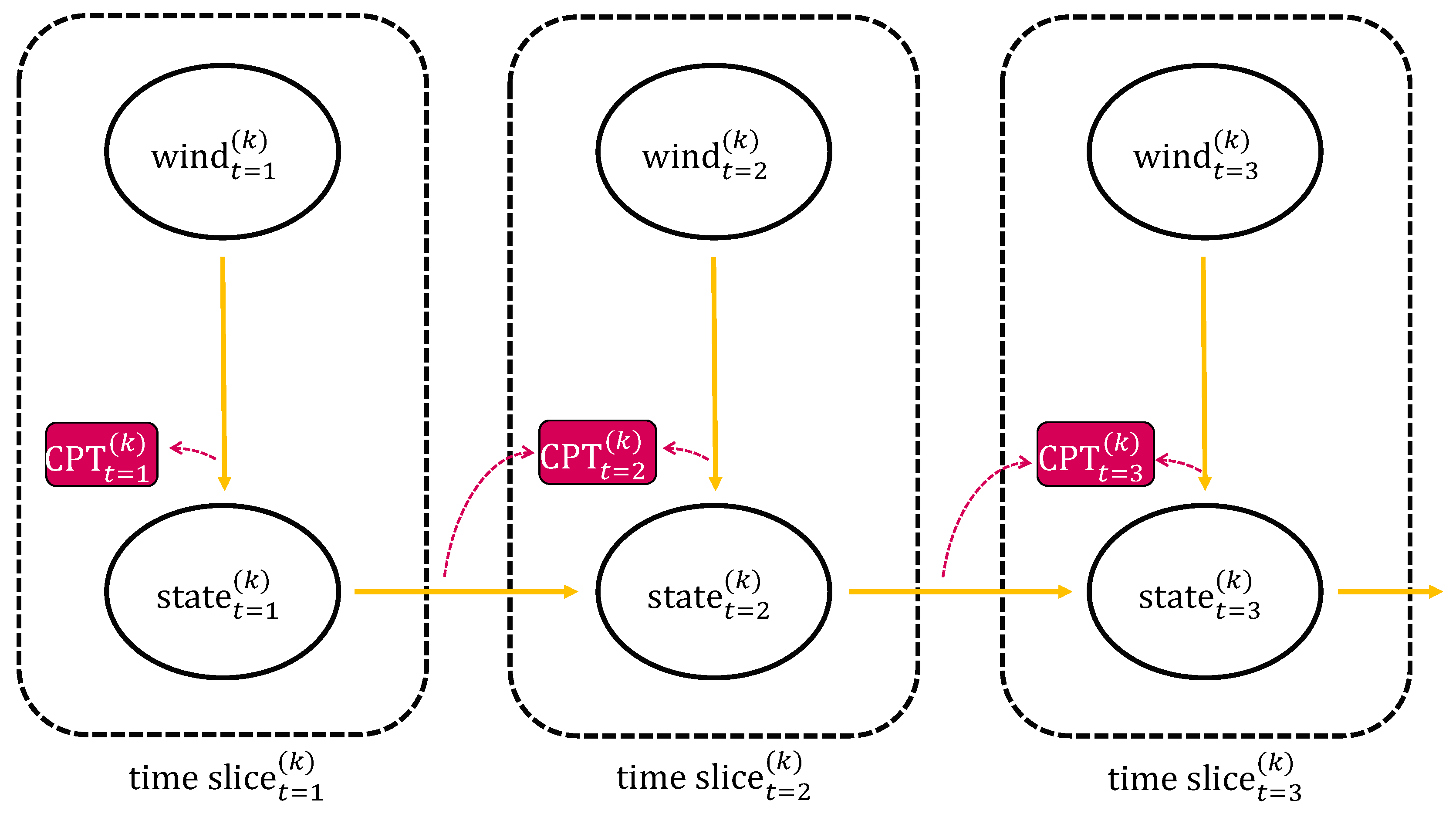
Figure 2.
Failure modelling.

Figure 3.
Network State Probability: One critical line with wind speed profile ‘A’.

Figure 4.
Network State Probability: Two critical lines with wind speed profile ‘A’.

Figure 5.
Network State Probability: Three critical lines with wind speed profile ‘A’.


Figure 6.
Wind speed spatial profiles.

Figure 7.
Network State Probability: Two critical lines with the wind spatial profile ‘B’.

Figure 8.
Network State Probability: Two critical lines with the wind spatial profile ‘C’.

Figure 9.
Long Run Simulation DBN-based.

Figure 10.
Proposed and future trend-approaches in transmission line modeling. (a) Wind spatial characterization on the network. Dotted red circle: proposed approach. Colored cell: Finer mesh approach. (b) Piece-wise line model with finer mesh approach.
Figure 10.
Proposed and future trend-approaches in transmission line modeling. (a) Wind spatial characterization on the network. Dotted red circle: proposed approach. Colored cell: Finer mesh approach. (b) Piece-wise line model with finer mesh approach.


Table 1.
Probability of wind speed.
| Weak | Medium | Strong | |
|---|---|---|---|
| wind |
Table 2.
CPT for .
| State | |||
|---|---|---|---|
| Run | Fault | ||
| wind | weak | ||
| medium | |||
| strong | |||
Table 3.
CPT for .
| State | ||||
|---|---|---|---|---|
| Run | Fault | |||
| state ∪ wind | Run | weak | ||
| Run | medium | |||
| Run | strong | |||
| Fault | weak | |||
| Fault | medium | |||
| Fault | strong | |||
Table 4.
Table Type Styles.
| Improved Markov Process | DBN | ||
|---|---|---|---|
| Critical Lines | Transition Matrix | Computation | Computation |
| Number | Dimension | Time [s] | Time [s] |
| 1 Line | 2 × 2 | 0.0008 | 0.1131 |
| 2 Lines | 4 × 4 | 0.001 | 0.1410 |
| 3 Lines | 9 × 9 | 0.010 | 0.1448 |
| 4 Lines | 16 × 16 | 0.012 | 0.1516 |
| 5 Lines | 32 × 32 | 0.017 | 0.1663 |
| 6 Lines | 64 × 64 | 0.083 | 0.1766 |
| 7 Lines | 128 × 128 | 0.102 | 0.2189 |
| 8 Lines | 256 × 256 | 0.400 | 0.1839 |
| 9 Lines | 512 × 512 | 2.010 | 0.2016 |
| 10 Lines | 1024 × 1024 | 8.664 | 0.3408 |
| 11 Lines | 2048 × 2048 | 49.79 | 0.3918 |
| 12 Lines | - | - | 0.8164 |
| 15 Lines | - | - | 3.160 |
| 20 Lines | - | - | 86.18 |
| 25 Lines | - | - | 3316 |
© 2020 by the authors. Licensee MDPI, Basel, Switzerland. This article is an open access article distributed under the terms and conditions of the Creative Commons Attribution (CC BY) license (http://creativecommons.org/licenses/by/4.0/).
Share and Cite
MDPI and ACS Style
Brugnetti, E.; Coletta, G.; De Caro, F.; Vaccaro, A.; Villacci, D. Enabling Methodologies for Predictive Power System Resilience Analysis in the Presence of Extreme Wind Gusts. Energies 2020, 13, 3501. https://doi.org/10.3390/en13133501
AMA Style
Brugnetti E, Coletta G, De Caro F, Vaccaro A, Villacci D. Enabling Methodologies for Predictive Power System Resilience Analysis in the Presence of Extreme Wind Gusts. Energies. 2020; 13(13):3501. https://doi.org/10.3390/en13133501
Chicago/Turabian StyleBrugnetti, Ennio, Guido Coletta, Fabrizio De Caro, Alfredo Vaccaro, and Domenico Villacci. 2020. "Enabling Methodologies for Predictive Power System Resilience Analysis in the Presence of Extreme Wind Gusts" Energies 13, no. 13: 3501. https://doi.org/10.3390/en13133501
Note that from the first issue of 2016, this journal uses article numbers instead of page numbers. See further details here.