Performance Simulation and Analysis of Occupancy-Based Control for Office Buildings with Variable-Air-Volume Systems

Abstract

Variable-air-volume (VAV) systems are used in many office buildings. The minimum airflow rate setting of VAV terminal boxes has a significant impact on both energy consumption and indoor air quality. Conventional controls usually have the terminal’s minimum airflow rate at a constant (e.g., 30% or more of the terminal design airflow rate), irrespective of the occupancy status, which may cause problems, such as excessive simultaneous heating and cooling, under ventilation, and thermal comfort issues. This paper examines the potential of energy savings from occupancy-based controls (OBCs). The sensed occupancy information, either occupant presence or people count, is used to determine the airflow rate of terminal boxes, the thermostat setpoints, and the lighting control. Using EnergyPlus, a whole-building energy modeling software, the energy savings of OBC strategies are evaluated for representative existing medium office buildings in the U.S. The simulation results show that the conventional OBC, based on occupant presence sensing, can save 8% of whole-building energy use in Miami (hot climate) for systems without air-side economizer and about 13% in both Baltimore (mixed climate) and Chicago (cold climate). Comparatively, the advanced OBC, based on people counting, can save 8% in Miami to 23% in Baltimore for systems with economizers. The outdoor-air fraction of the supply air from air-handling units significantly affects the potential energy savings from the advanced OBC strategy. In addition to energy savings, the advanced OBC satisfies the zone ventilation during all occupied hours over the whole year.

1. Introduction

Variable-air-volume (VAV) systems are one of the most widely used heating, ventilating, and air-conditioning (HVAC) systems in commercial buildings. According to a building characteristics analysis based on the most recently published Commercial Buildings Energy Consumption Survey [1], buildings with VAV systems represent 43% of all U.S. commercial building floor space [2]. That percentage is even larger for office buildings, 86% for those greater than four stories and 55% for those with 2~4 stories. Among different VAV system configurations, the single-duct, multi-zone VAV system is one of the most popular systems [3]. In a single-duct, multi-zone VAV system, outdoor air (OA) enters the air-handling unit (AHU) through an outdoor-air damper and is mixed with the recirculated return air from the spaces, often with the assistance of a fan in the return duct. The mixed air sequentially passes through a filter, a heating coil (if present), and a cooling coil, which are used to condition the supply air to a predefined temperature setpoint in the supply duct downstream of the supply fan. The supply-fan speed is modulated to maintain the supply-air static pressure at a setpoint. Several methods, such as direct measurement, fan tracking, and mixed-air-plenum-pressure control, can be used to control the minimum OA flow rate in VAV systems [4], but they all have strengths and weaknesses in field implementations.

A VAV system also includes air terminal units as the last flow rate and temperature control device before conditioned air from the system enters each of the thermal zones. There are many different types of VAV terminal units (e.g., throttling, fan-powered, and induction) though the rest of this paper focuses on VAV throttling terminal boxes. Each terminal box serves a building zone (which can be a single room or multiple rooms), controlling the airflow rate to the zone and reheating the air when it is too cool for the zone served. VAV terminal boxes work in one of three operating modes: cooling, deadband, and reheating. The specific mode of operation depends on the zone temperature, which is ordinarily measured by a thermostat in the zone. The VAV box operates in the cooling mode when the zone-air temperature rises above the cooling setpoint for the zone. The terminal box varies the airflow rate in the cooling mode by modulating the terminal damper opening. The VAV box operates in the deadband mode when the zone-air temperature lies between the space cooling and heating setpoints. In this mode, the terminal box controller maintains the airflow rate at its minimum setting to provide zone ventilation. The VAV box enters the heating mode when the zone-air temperature falls below the space heating setpoint. In this mode, the heating capacity is modulated to meet the space heating load. When a single-maximum control logic is used, the airflow rate is maintained constant at its minimum setting while the reheating coil valve (if hot water is used) is modulated. When a dual-maximum control logic is used, the airflow rate is initially maintained at its minimum setting but after the discharge-air temperature reaches the upper limit, the airflow rate is then modulated open towards the maximum setting for heating to meet the heating need [5].

Terminal boxes are sized to satisfy the thermal design load (usually the cooling load) of the zones they serve [6]. The terminal box’s minimum airflow rate setting has significant impacts on energy consumption to condition the zone served and the zone’s indoor air quality. In principle, the value of this parameter needs to be determined as the larger value between the airflow rate required to satisfy the heating load and the airflow rate required for ventilation. However, in practice, control system integrators and installers commonly use a rule-of-thumb setting for the minimum airflow rates of terminal boxes, say, 30%~50% of the maximum airflow rates to satisfy the ventilation requirement [7,8]. Furthermore, once established, this minimum airflow rate setpoint is generally held constant during system operation, which potentially leads to two major ventilation issues. First, the rule-of-thumb setting cannot guarantee that the zone OA ventilation requirement is satisfied, as will be shown later in the paper. Second, because building occupancy varies dynamically over time, using a constant minimum airflow rate can result in over-ventilation during times when the zone has less than maximum occupancy or is unoccupied. Over-ventilation causes energy waste and even discomfort for occupants in some spaces (e.g., conference rooms) from over-cooling [9,10].

To cope with variations in occupancy, current ASHRAE Standard 62.1 [11] allows dynamic reset of outdoor airflow rate in response to changes of zone occupancy, including an occupancy standby mode to temporarily shut off the zone ventilation. The Standard also lists four measures that can be used to estimate the number of occupants: (1) Direct count of people, (2) presence of people, (3) time-of-day schedule, and (4) CO₂-based occupancy estimation. The first measure counts the number of occupants in a space using technologies, such as image recording, radio frequency identification tags, passive infra-red sensors, and acoustic sensors [12]. The second measure simply detects whether a space is occupied or not by using any of many well-developed commercial technologies, such as passive infrared and motion sensors. The third measure of using a time-of-day schedule estimates the number of occupants using a predefined peak number of occupants and a temporal occupancy profile. This measure is appropriate for spaces (e.g., classrooms) for which the occupancy schedule varies little or in an easily predicted manner. However, offices, for example, ordinarily do not have such occupancy characteristics, and thus, are not suitable for the use of time-of-day schedules to determine the number of occupants. The fourth measure of using CO₂ concentration involves calculating the number of occupants based on a steady-state equation by assuming the CO₂ generation rate of people is a constant. Use of CO₂ concentration for people counting introduces several complications [13]: (1) The space CO₂ concentration seldom reaches steady state; (2) the CO₂ generation rate can vary widely with occupant activity levels; (3) CO₂ sensor accuracy degrades with time; and (4) there is a time lag of 10 to 20 min between each occupancy change and the corresponding CO₂ concentration change in the space.

Although it is not a common practice to use CO₂ concentration for occupancy estimation, CO₂ has been used as a surrogate for the concentration of human bioeffulants to control OA flow intake rate, which is known as CO₂-based demand-controlled ventilation (DCV) in literature. DCV for single-zone systems has been well studied [14,15,16,17], with the basic concept of modulating the OA damper of air-handling units to maintain the space CO₂ concentration below a specified limit (e.g., 1000 ppm). Regarding DCV for multi-zone VAV systems, Nassif et al. [18] proposed the modulation of OA intake to maintain the supply-air CO₂ concentration low enough to sufficiently dilute CO₂ generated in a critical zone (i.e., the zone requiring the highest percentage of OA). Murphy [19] discussed two control approaches for using CO₂ concentration for multi-zone ventilation reset. The first approach used the CO₂ concentration in critical zones to vary the amount of OA intake at the AHU. The second approach used the sensed CO₂ concentration to reset the ventilation requirement in critical zones, based on which the system ventilation efficiency and the required OA flow at the AHU were then calculated. Lin and Lau [20] proposed a CO₂-based DCV strategy that reset the system OA flow rate by strictly following the procedure of solving the multi-zone system equations according to ASHRAE Standard 62.1. In contrast to previous studies that focused on the system OA reset at the AHU, Kang et al. [21] used CO₂ concentration to reset the VAV terminal airflow rate by opening the terminal damper wider if the CO₂ concentration was above its upper limit and closing the damper further otherwise with the consideration of a control deadband. In case the CO₂ concentration was still beyond the upper limit after the terminal damper had been fully open, the outdoor air intake at the AHU was increased.

In this paper, we examine how much energy can be saved by control algorithms that use occupancy information. Specifically, our focus is on rule-based control algorithms that can be simply applied to VAV systems in existing office buildings. The sensed occupancy information, either occupant presence or people count, is used to determine the airflow rate of terminal boxes, the thermostat setpoints, and the lighting level. We hereinafter refer to the sensors for occupant presence (occupied or unoccupied) as conventional occupancy sensors, and the sensors used to detect the number of occupants as advanced occupancy sensors. Occupancy-based control (OBC) strategies based on these two kinds of sensors are proposed and evaluated using building simulation. Their results are compared with the baseline of not using occupancy sensors. In the rest of this paper, previous related work is reviewed in Section 2. The office building model used to evaluate the impacts of occupancy-based controls is discussed in Section 3. Occupancy modeling and occupancy-based control strategies are discussed in Section 4 and Section 5, respectively. Simulation results and their implications are discussed in Section 6, and Section 7 concludes the paper with possible directions to extend this work.

2. Previous Related Work

Many OBC strategies have been proposed and evaluated in the literature. Two common categories of approaches investigated for OBC are rule-based control and model predictive control (MPC). A rule-based approach makes control decisions based on simple algorithms derived from the understanding of how the physical system operates and are more widely understood by building staff. In contrast, an MPC uses data-driven models to project system behavior over a future time horizon, is mathematically more complex than rule-based controls, but can yield better results in many cases when the models accurately represent actual behavior.

Rule-based control requires instantaneous occupancy measurements (presence/absence or number of occupants) to calculate the control outputs. The sensed occupancy information, together with other measurements (e.g., space air temperature), are used as input signals to override the ordinary control settings. For example, Balaji et al. [22] leveraged the occupants’ mobile devices to detect which rooms are occupied. The thermostat setpoints were relaxed by 1.1 °C if the room is unoccupied. Based on a one-day experiment in a university campus building, electric energy savings of 17.8% for HVAC systems were achieved from the application of occupancy-based controls for 23% of the zones in the building. Goyal et al. [23] used measured occupancy to calculate and reset the minimum airflow rates of VAV terminal boxes. The temperature setpoints were relaxed when zones were unoccupied. Based on the MATLAB simulation for a single zone in three typical days (i.e., cold, hot, and mild), Goyal et al. found HVAC energy savings of approximately 50% for that zone, relative to the baseline terminal control that had a minimum airflow rate fixed at 40% of the terminal box design flow rate. This rule-based OBC strategy was further tested in a campus building in Gainesville, FL [24]. The field test was performed on 12 fully actuated zones (i.e., each zone is served by a single terminal box) for six consecutive days in April. The experimental results showed that the rule-based OBC achieved 37% HVAC energy savings—30% of which came from heating, while the rest from cooling and fan. Zhang et al. [25] distinguished space types (i.e., private office, open-plan office, and conference room) when proposing rule-based OBC strategies for VAV terminal box controls and lighting controls. Using EnergyPlus simulation, they modeled their OBC strategies for a prototype large office building across 15 different climate zones of the U.S. At a national scale, 17.8% average annual energy savings as a fraction of whole-building energy use were found for OBC using advanced occupancy sensors and 5.9% for OBC using conventional occupancy sensors.

Model predictive control (MPC) is an approach based on optimal control, which requires the prediction of occupancy (presence/absence or the number of occupants) at future times and solves an optimization problem to determine the control inputs. These control inputs are implemented at the current time $t_k$, and their corresponding outputs are measured. Using the measured outputs, the control inputs at the next time $t_{k+1}$ are calculated by solving the optimization problem again for the next $K$ time steps. To solve the optimization problem, MPC requires a dynamic model and the prediction of exogenous inputs, such as weather and occupancy. Oldewurtel et al. [26] compared various types of MPC strategies for the control of lighting, window blinds, and HVAC in an office building. Their simulation results showed that the MPC based on perfect prediction over a 3-day time horizon had a savings potential of up to 34% of whole-building energy use if five out of 15 days are vacant on the average. A large portion of this savings potential could be captured by using the default occupancy schedule as the prediction and adjusting lighting and ventilation to instantaneous measurements of occupancy status. Similar observations were made in another study [23], where the MPC controller using perfect occupancy prediction over a 24-hour time horizon led to an additional 1–13% HVAC energy savings relative to the baseline without OBC. Accounting for the challenge of perfect occupancy prediction and the efforts to implement MPC, Goyal et al. [23] concluded that rule-based feedback control would be most suitable for occupancy-based zone-climate control. If the ventilation requirement were relaxed for unoccupied spaces and close to perfect occupancy predictions were available, the savings from MPC would increase substantially, potentially making use of MPC cost-effective.

This paper extends the previous work by Zhang et al. [25] to estimate the energy savings of rule-based OBC strategies using the whole-building simulation program EnergyPlus [27]. Major extensions include simulation model changes and refinements as summarized below:

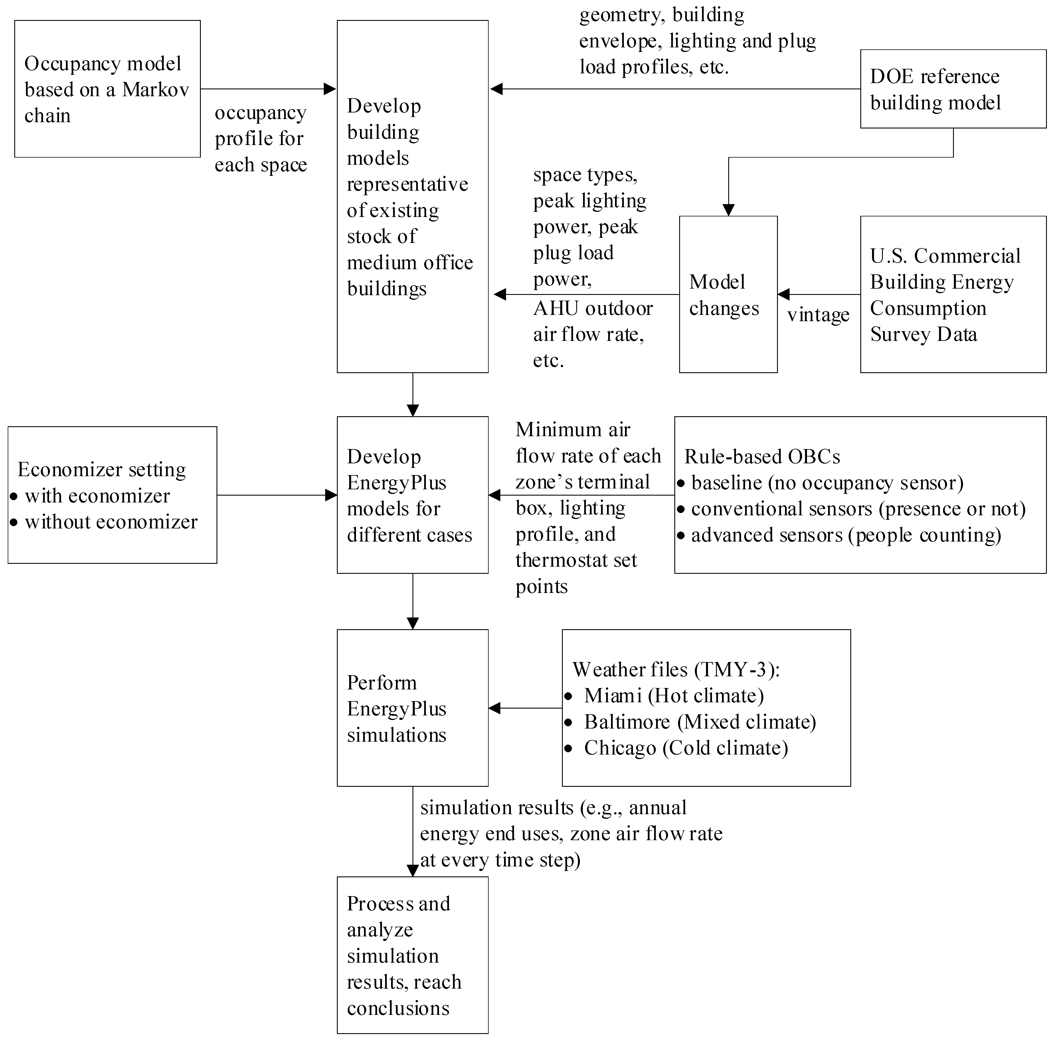
• Instead of using the large office building model, the medium office building model from the U.S. Department of Energy Commercial Reference Building Models [28] is used in this work;
• Instead of using a constant predefined occupancy schedule for all offices and another one for all conference rooms, a stochastic occupancy model is used in this work to generate an occupancy profile for each zone;
• Instead of keeping a constant OA flow rate into the AHU, a constant OA fraction of the AHU airflow rate is assumed in this work to reflect the most prevalent practice of setting the minimum OA damper position under the design conditions [6,29];
• Due to the limitation of EnergyPlus simulation capabilities when the previous work [25] was performed, there were two issues on modeling ventilation control. First, for the zones consisting of private offices, the probability of being unoccupied at hour $i$ was estimated as ${\left(1-P_{office,i}\right)}^3$, assuming that each zone had three private offices and where $P_{office,i}$ is the probability of an average office being occupied during hour i, which is estimated as a static value corresponding to an occupancy profile from the literature. Second, in the implementation of OBC based on occupant count, the VAV box minimum airflow rate was reset using linear interpolation between 0 and the baseline minimum setting (i.e., 50% and 30% of design flow rate for conference rooms and offices, respectively) according to the current occupancy. For example, if the fraction of peak occupancy is 0.5 for a conference room at a specific hour, the minimum airflow rate for the corresponding terminal box is set as 25% (=0.5×50%) of the design airflow rate. The implicit logic behind this approach is that the ventilation requirement is proportional to the number of occupants, which is not valid because of the existence of an area component of the required ventilation. Both drawbacks are addressed in this work through the enhanced modeling capability of EnergyPlus in recent releases;
• More efforts are made to investigate the impact of system OA fraction and air-side economizer setting on the energy savings of OBC strategies.

3. Methodology

The methodology used in this study is depicted in Figure 1. Because the purpose is to use simulation to evaluate the potential for energy savings from OBC, we develop a building model representative of the existing stock of medium office buildings in the United States. The U.S. Department of Energy (DOE) commercial reference building models [28] are the basis of the model developed. Building geometry, floor area, building envelope construction and profiles of internal heat gains (i.e., lighting and plug loads) are directly from the reference building model. Data from the U.S. Commercial Building Energy Consumption Survey [1] determines the average vintage of the existing medium office building, based on which some changes are made to align the reference model to currently standing medium office buildings. The major changes include detailed space types, which determine ventilation needs, peak lighting power and peak plug load power, which affect HVAC equipment sizing, and AHU outdoor airflow rates, which affect the terminal airflow rate required to meet ventilation needs. The Markov-chain-based occupancy model of Page et al. [30] is adapted to create a unique annual 15-min occupancy profile for each zone. After the building models are developed for three locations with different climates, they are perturbed to support varied controls, including two economizer controls (i.e., with and without air-side economizer) and three occupancy-related controls (i.e., baseline without the use of occupancy sensors, the use of conventional sensors to detect occupant presence or not, and the use of advanced occupancy sensors to count the number of occupants in each zone). All models are simulated with EnergyPlus software and the Typical Meteorological Year 3 (TMY-3) weather files. Output files from EnergyPlus simulations are post-processed to obtain results, which are interpreted to develop the findings on the energy-saving potential of OBC.

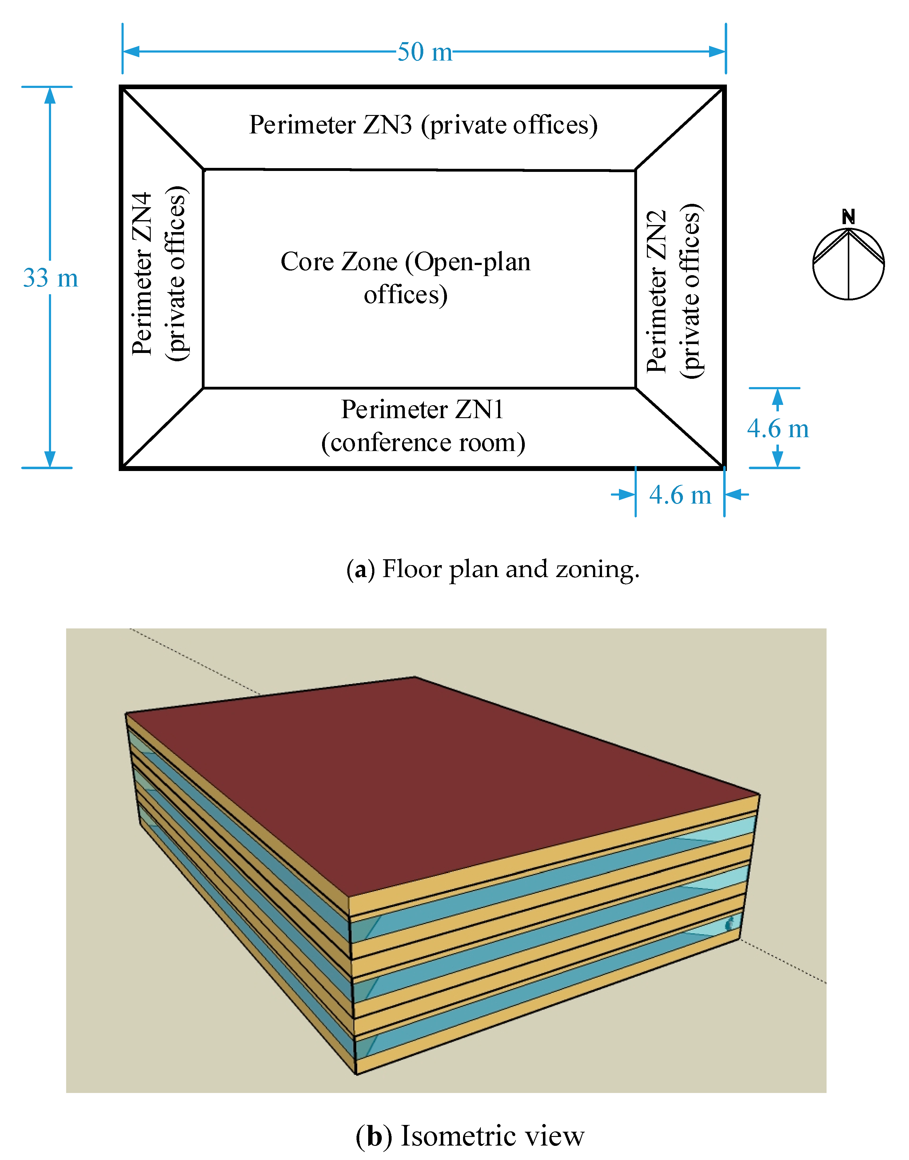
4. Building Model Description

The medium office building model originates from the commercial reference building models developed by the U.S. Department of Energy [28]. The reference building models offer three vintages: New construction in compliance with ASHRAE Standard 90.1-2004 [31], existing buildings constructed in or after 1980, and existing buildings constructed before 1980. According to the latest U.S. commercial building energy consumption survey [1], the median age of office buildings in the U.S. was approximately 23 years in 2012. By assuming that this median age has not changed appreciably between 2012 and 2019 (when the paper was prepared), the median year in which currently standing medium office buildings were built is 1996. Ideally, the building modeled to estimate likely energy savings from retrofit with OBC would be the average medium office building built in 1996, but in its 2019 condition. Such a requirement, however, cannot be met by any of the three vintage models of reference buildings. Thus, an alternate procedure [25] is used to define a representative medium office building for this study. Starting with the reference medium office building model for new construction, adjustments are made to bring the model closer to the characteristics that might be expected for a building constructed in 1996, but that has been upgraded over the last 23 years. The changes (see

Table 1. Changes to the medium office building reference model to create a building model that approximates a medium office building constructed in 1996 as it would exist in 2019 and the rationale for each change.

Category	Changes Made	Rational
Zone description	Specific space types (conference room, private office, and open-plan office) were assigned to the thermal zones.	The use of distinct space types enables evaluation of the savings associated with occupancy-based control (OBC) based on the unique occupancy patterns and ventilation requirements of different spaces.
	The occupancy profiles were modified for private offices, open-plan offices, and conference rooms to consider spatial and temporal variations.	To address the problem of using static typical occupancy profiles to represent all occupants for a whole year.
Heating, ventilating, and air-conditioning system (HVAC) sizing	Terminal-box sizing factor (flow rate and reheat) was increased from 1.0 to 1.2.	The larger size for the terminal boxes more realistically represents a late 1990s office building.
	Lighting peak load power density (LPD) was scaled to 133% of the LPD required by Standard 90.1-2004 for HVAC sizing. The LPD for calculating lighting energy consumption was unchanged from the reference model.	HVAC systems in a late 1990s building would have been sized for the less efficient lighting of the era. Lamps and lighting fixtures are assumed to have been replaced with more efficient ones since building construction in 1996, but retrofit of HVAC components, primarily the terminal boxes, is assumed to have been considered too expensive to have been replaced in most buildings.
	Peak plug load density was scaled to 140% of the Standard 90.1-2004 prototype plug load density for HVAC sizing. Plug load density for modeling energy consumption was unchanged from the reference model.	HVAC systems in late 1990s buildings would have been sized for the higher plug load densities of that era. Expensive HVAC system replacements, such as for terminal boxes, are less likely to have been done.
Outdoor airflow rate at air-handling units	The outdoor airflow rate was changed from a constant (sum of zone outdoor air requirements) to 25% of supply airflow rate.	Outdoor-airflow stations are not commonly used on air-handling units (AHUs) in the field.
Terminal box settings	The minimum airflow rate for conference rooms was changed from 30% to 50% of the design peak flow rate.	Implementation of this procedure is based on common practices for conference room minimum damper positions presented by [8,32].
	The control of maximum discharge air temperature was added.	The discharge air temperature from terminal boxes should be kept below a certain limit to avoid stratification and short circulation of conditioned air.

) are, thus, made mostly based on the authors’ professional judgment because of the lack of reliable and unified specifications on office building retrofits.

The resulting model represents a three-story office building with approximately 5000 m² of total floor area. Figure 2 illustrates an axonometric view of the building and its thermal zoning. The building has 1.2-m-high plenum spaces above each floor and a continuous band of windows for a total window-to-wall fraction of 33%. Details on building envelope construction and the associated thermal-physical properties of materials can be found in [28]. The perimeter zones are delineated by the orientation of each façade. Each perimeter zone is 4.6 m deep from its exterior walls. On each floor, perimeter zone 1 (Figure 2) is used as the conference room while each of the other three perimeter zones consists of multiple private offices, and the core zone is open-plan offices.

Table 2. Design occupancy densities and ventilation rates.

Space Category	Occupant Density for Ventilation Design	People Outdoor Air Rate (Rp)	Area Outdoor Air Rate (Ra)
	# People per 100 m2	m3/s/person	m3/s/m2
Office	5	0.0025	0.0003
Conference	50	0.0025	0.0003

lists the design occupant densities and ventilation requirements, which follow ASHRAE Standard 62.1-2004 [33]. Typical office work with a metabolic rate of 120 W per person and typical clothing insulation (0.5 Clo from in the summer and 1 Clo in the winter) are modeled. Detailed model inputs can be found in [28].

Three packaged direct-expansion rooftop VAV air-conditioning units with gas furnaces serve the medium office building, one for each floor. Persily et al. [29] conducted a ventilation field study for U.S. office buildings and found that for those AHUs without economizers (1) the mean ratio of the design OA flow rate to the total design supply airflow rate is 0.19 and (2) the mean ratio of the measured OA intake to the design OA intake rate is 1.37. Based on these values, the mean OA fraction of the AHU design airflow rate is approximated to be 25%. Therefore, the AHUs are simulated in the model to have their minimum OA flow rate set at a fixed 25% of the supply airflow rate. Pressure-independent VAV terminal boxes are used in the model. The maximum airflow rate of each VAV box is automatically sized (autosized) by EnergyPlus based on the zone thermal load at design conditions. Following common practice and design recommendations [34], all terminal boxes in the model have hot-water reheat and the single-maximum control logic. The minimum airflow rate is set at 30% of the maximum for terminal boxes serving offices and at 50% for those serving conference rooms. The scheduled system operation hours are from 06:00 to 20:00 on weekdays and from 06:00 to 18:00 on Saturdays, with the first two hours for space warming up or cooling down. During these operation hours, the zone thermostat setpoints are 23.9 °C for cooling and 21.1 °C for heating. A 5.6 °C setback for heating and set up for cooling is used during scheduled system off-hours.

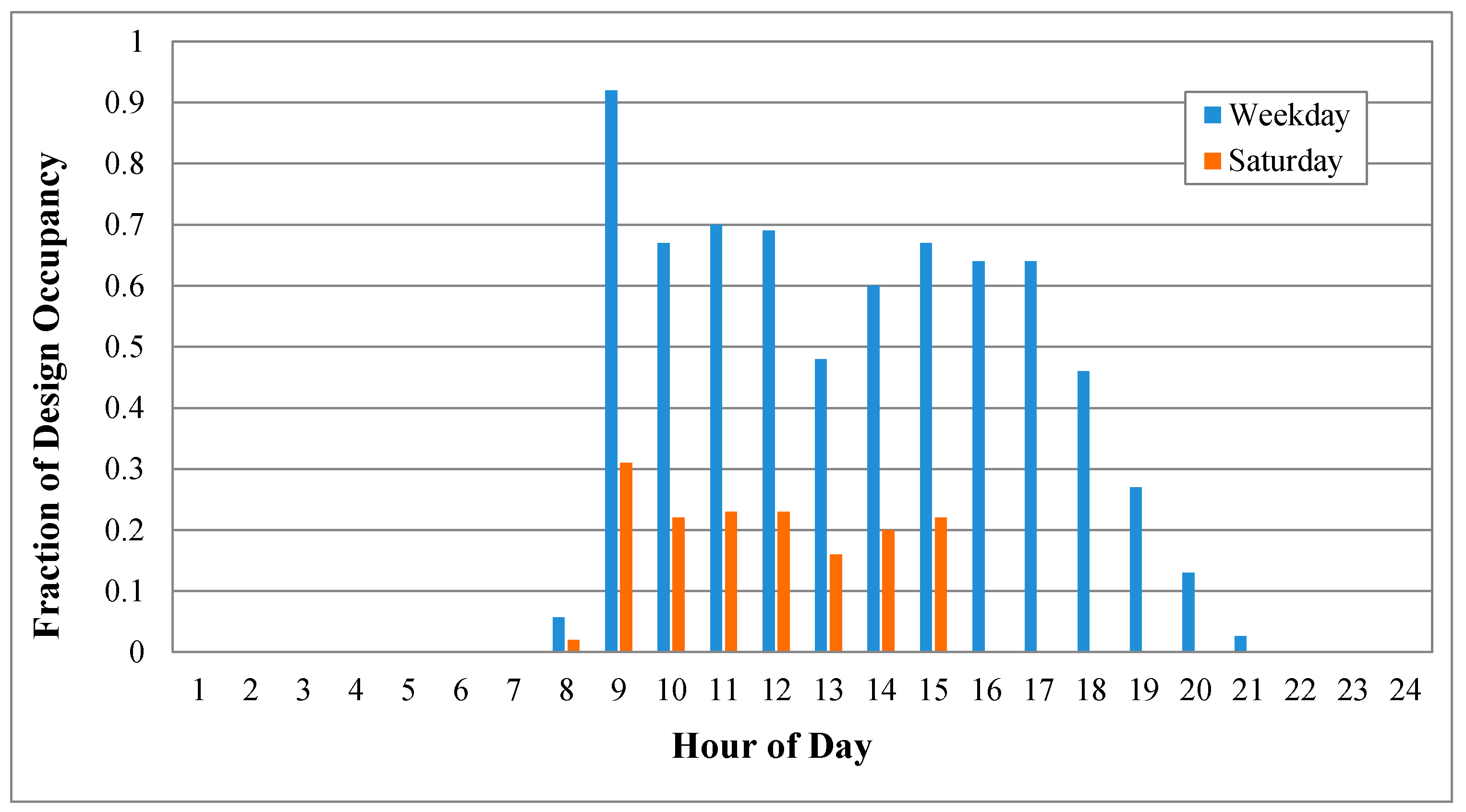
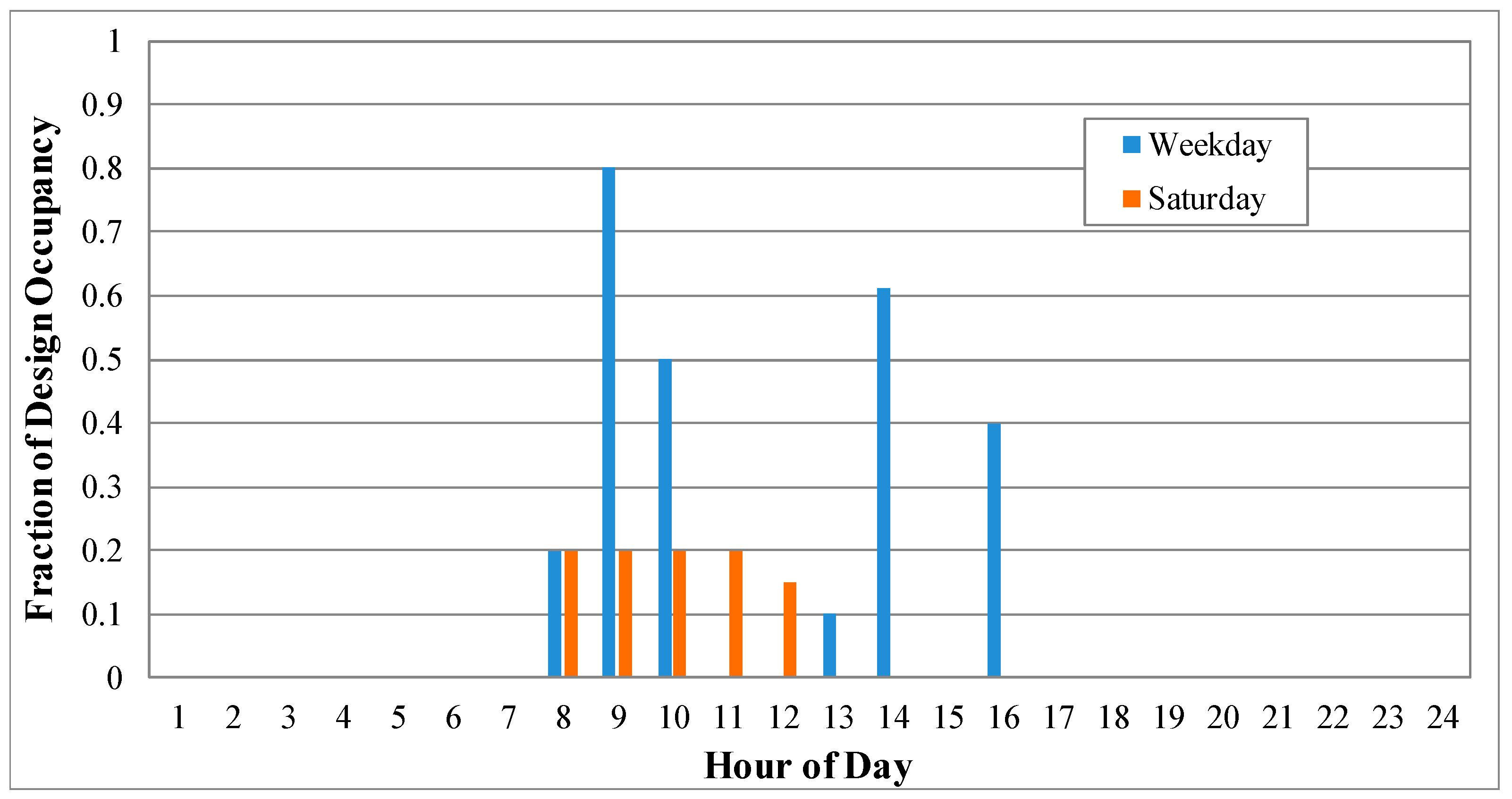
5. Occupancy Modeling

Realistic modeling of occupancy is critical to the evaluation of OBC strategies. The most common approach of considering occupancy in building energy simulation programs is using occupancy profiles. Daily occupancy profiles are usually defined differently on weekdays and weekends for office buildings. A daily profile (either for a weekday or weekend) consists of 24-hourly values, each of which corresponds to a fraction of the design (maximum) occupancy. The same weekday and weekend daily profiles are repeated throughout the entire year for all occupants in each space type (i.e., office or conference room). Using this simplified approach to study occupancy-based controls has the following weaknesses. First, the day-to-day temporal variations of occupancy pattern (e.g., attributable to late arrivals, early departures, and unpredicted absences on weekdays) are mostly neglected. Second, the spatial variation of the occupancy pattern is neglected, but the reality is that actual occupancy profiles vary with different spaces even when they belong to the same space type (e.g., office). To address the problems of using repetitive occupancy profiles, the stochastic model for simulating occupant presence from Page et al. [30] is employed in this work.

The Page model [30] simulates occupant presence as an inhomogeneous Markov chain with probabilities of transition $T_{ij}\left(t\right)$ from state i to state j defined as:

$$T_{ij}\left(t\right)=Probability\left(X_{t+1}=i|X_t=j\right)$$

(1)

where $X_t$ is the state variable of occupant presence at time step $t$, and $i$ and $j$ take binary values, with 0 for absence and 1 for presence. Thus, T₀₁ is the transition probability from occupant being absent to present, and T₁₁ is the probability of the state remaining occupied.

Based on the profile of probability of occupant presence and the parameter of mobility ($\mu$), which is defined as the ratio of the probabilities of state change and of no change, the time-dependent conditional probability in Equation (1) can be further expressed as [30]:

$$T_{01}\left(t\right)=\frac{\mu -1}{\mu +1}P\left(t\right)+P\left(t+1\right)$$

(2)

$$T_{11}\left(t\right)=\frac{P\left(t\right)-1}{P\left(t\right)}\left[\frac{\mu -1}{\mu +1}P\left(t\right)+P\left(t+1\right)\right]+\frac{P\left(t+1\right)}{P\left(t\right)}$$

(3)

In Equations (2) and (3), $P\left(t\right)$ and $P\left(t+1\right)$ are the probabilities of presence, respectively, at time steps$t$ and $t$+1. Their values are from the predefined occupancy profiles as illustrated in Figure 3 and Figure 4, where the occupancy profile for offices is from Wang et al. [35], while the profile for conference rooms is from Hart [36]. Page et al. [30] suggested defining constant values for three levels of mobility (low, medium, and high), but the values were not given. This paper uses a value of 0.25 for $\mu$, the mean value used by Gunay et al. [37] when comparing different occupancy models.

The Page occupancy model simulates the presence pattern of each occupant individually. To obtain the occupancy pattern for a zone, each occupant in that zone is simulated separately, and the produced patterns of presence are then summed. For example, the peak number of occupants in Zone 2 is calculated to be seven, based on the zone geometry (Figure 2) and the design occupant density (Table 2). The Page occupancy model needs to be run seven times to obtain that zone’s occupancy profile. The outcome of occupancy modeling includes the occupancy patterns for all 15 zones, which are different from each other. All occupancy patterns have a time interval of 15 min, instead of one hour as used in traditional occupancy profiles. The generated annual occupancy patterns are used as the inputs to the EnergyPlus simulation program.

6. Control Strategies and Simulation

We now describe the baseline control and the two occupancy-based control strategies (one for conventional occupancy sensors that detect presence only and the other for advanced occupancy sensors that detect the number of occupants). These control strategies differ in the following respects: (1) The minimum airflow rate settings of terminal boxes, (2) the zone thermostat setpoints, and (3) the lighting control.

6.1. Baseline Control

The baseline control does not rely on occupancy information at all. Thus, the terminal box has a constant minimum airflow rate setting (i.e., 30% of the maximum airflow rate for offices and 50% for conference rooms) and implements a single-maximum control logic. As a result, the airflow rate from each terminal box is adjusted between its maximum and minimum settings to match the cooling load as conditions change. The terminal box has its airflow rate at the minimum setting when the zone is in the deadband mode and the heating mode. During the deadband mode, the reheat coil valve is closed. During the heating mode, the reheating coil valve modulates open until the zone temperature is increased to the heating setpoint. The thermostat setpoints in all zones follow the same schedule as defined in Section 2 (see

Table 3. Comparison of the baseline control and OBC strategies.

Control Characteristics, Parameters and Applicable Space Types		Baseline	Conventional OBC	Advanced OBC
Minimum terminal airflow setting (% of the peak design airflow rate)	Private offices	30%; single-maximum control	30% when any of the offices in the zone served is occupied and 0 when all offices are unoccupied; dual maximum control	30% when any of the offices in the zone served is occupied and area ventilation when all offices are unoccupied; dual maximum control
	Open-plan offices	30%; single-maximum control	30%; single-maximum control	The minimum is calculated dynamically based on the occupant count and the area ventilation; dual maximum control
	Conference rooms	50%; single-maximum control	50% when occupied and 0 when unoccupied; dual maximum control	The minimum is calculated dynamically based on the occupant count and the area ventilation; dual maximum control
Thermostat setpoints during scheduled building operation hours	Private offices	21.1 °C for heating and 23.9 °C for cooling	Same as baseline	20 °C for heating and 25 °C for cooling when all offices in the zone are unoccupied; otherwise the same as baseline
	Open-plan offices	21.1 °C for heating and 23.9 °C for cooling	Same as baseline	Same as baseline
	Conference rooms	21.1 °C for heating and 23.9 °C for cooling	20 °C for heating and 25 °C for cooling when the conference room is unoccupied; otherwise the same as baseline	20 °C for heating and 25 °C for cooling when the conference room is unoccupied; otherwise the same as baseline
Lighting	Private offices	No occupancy-based lighting control	Lights are turned off after 15-minute time delay when the space is unoccupied.	Lights are turned off after 5-second time delay when the space is unoccupied.
	Open-plan offices	No occupancy-based lighting control	No occupancy-based lighting control	No occupancy-based lighting control
	Conference rooms	No occupancy-based lighting control	Occupancy-based common lighting controls with 15-minute time delay	Occupancy-based advanced lighting controls with 5-second time delay

). Similarly, interior lighting follows a general schedule for office buildings, as shown in Figure 5 [28], where the hourly values indicate the fraction of peak lighting power density.

6.2. Conventional OBC

The conventional OBC modifies the baseline control depending on the space type and the space occupancy status. Major changes relative to the baseline control include the following (see also Table 3):

• Terminal box minimum airflow rate settings. For private offices and conference rooms, the minimum airflow rate is reset to zero when no people are detected in any of the spaces served by the terminal box. Accompanying the change of minimum terminal airflow rate, the dual-maximum control logic replaces the single-maximum control logic used in the baseline. As a result, the zone heating load may trigger a higher airflow rate than the minimum setting. Note that for open-plan offices, the minimum airflow rate is kept at the same value as for the baseline control because the probability of large open-plan offices being unoccupied is relatively low;
• Thermostat setpoints. For conference rooms, the thermostat setpoints are reset to 25 °C for cooling and 20 °C for heating when the space is unoccupied. Although some time delay (say 15 min) is generally needed in the field to reset thermostat setpoints after the space is detected to be unoccupied, it is not considered in the simulation. The thermostat setpoints are not reset for offices;
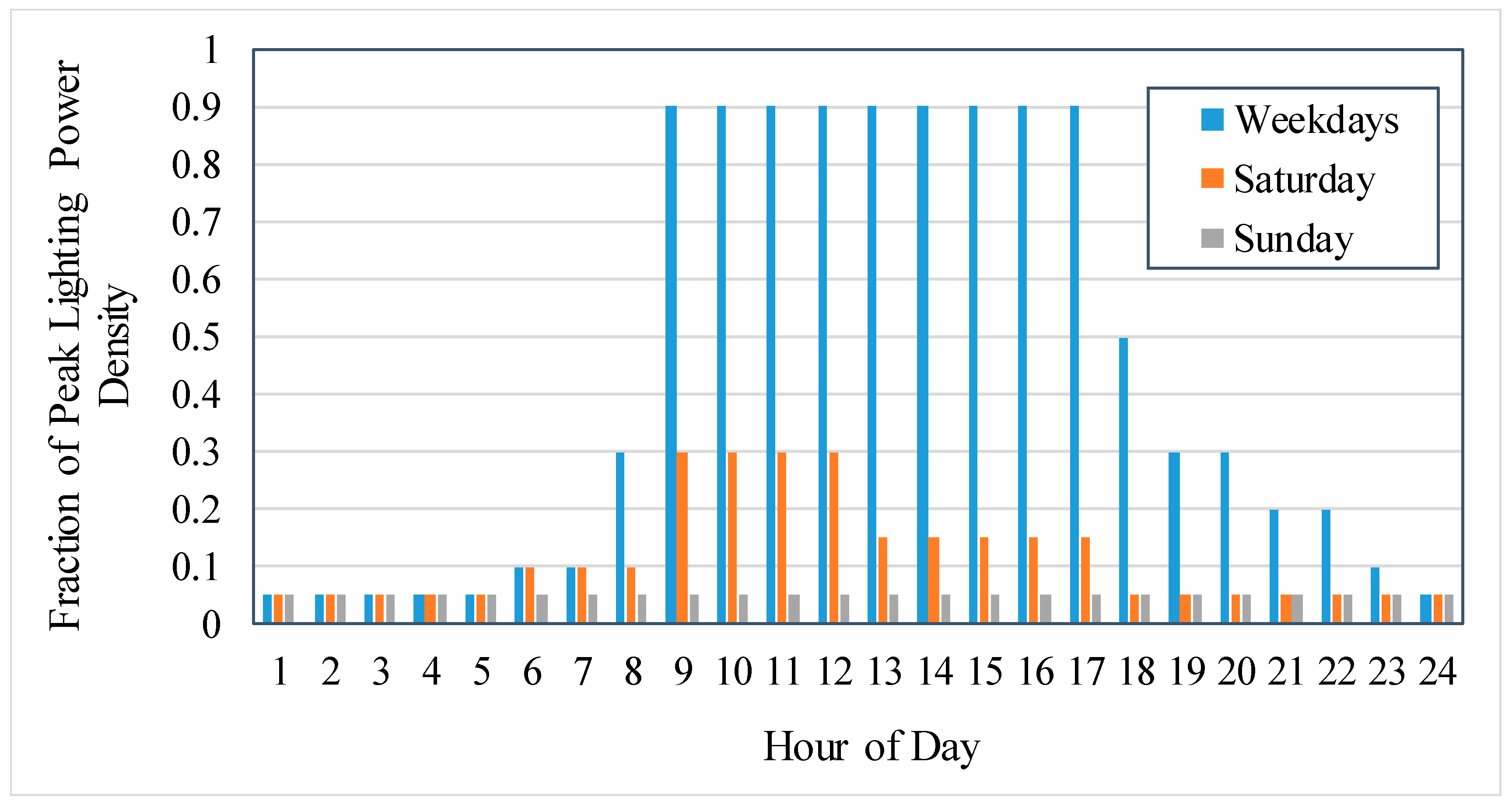
• Lighting control. In conventional OBC, lights are on when occupants enter a room and are off following a time delay after all occupants have left the room. Delay times of approximately 15 min are usually used to help ensure that lights do not turn off while occupants are still in the room. Lighting controls are applied in conference rooms and private offices. Von Neida et al. [37] investigated the potential of lighting energy savings in different space types by applying occupancy-based lighting control with varied delay times. About 24% of lighting energy savings were obtained for both conference rooms and private offices for a time delay of 15 min. To consider occupancy-based control for lighting in the simulation, the lighting schedule during building operation hours (08:00 to 22:00) is revised using the following equation:

$$LP{F}_{OBC, i}=LP{F}_{base, i}\ast \left(1-F_{savings}\right)$$

(4)

where $LP{F}_{OBC,i}$ and $LP{F}_{base,i}$ refer to the fraction of peak lighting power density at hour $i$ for the case of occupancy-based lighting control and baseline control, respectively. The fractional energy savings, $F_{savings}$, takes the value of 24% for conventional OBC. As an example, Figure 5 shows the baseline lighting being 0.9 of the peak lighting power density from 08:00 to 17:00 during weekdays. The lighting power fraction is changed to $0.9\times \left(1-0.24\right)=0.684$ during the same hours for the conventional OBC simulation.

6.3. Advanced OBC

The advanced OBC improves on the conventional OBC by controlling ventilation based on the number of occupants detected in spaces. Major differences relative to conventional OBC are highlighted in the following (see also Table 3):

• Minimum terminal airflow setting. The zone outdoor airflow rate required at any time t ($V_{oz,t}$) is calculated as:

  $$V_{oz,t}=\frac{R_p{P}_{z,t}+R_a{A}_z}{E_z}$$

  (5)

  where $R_p$ and $R_a$ represent the OA flow rates required per person and per floor area, respectively, as indicated in Table 2, $A_z$ is the zone floor area in m², $P_{z,t}$ is the number of occupants at time $t$, and $E_z$ is the zone air distribution effectiveness. In this work, the value of 1 is used for $E_z$ in the simulations because the discharge air temperature does not exceed the space temperature by more than 8 °C for most times.

The zone supply airflow rate ($V_{pz,t}$), including both OA and recirculated air, needed to meet the ventilation requirement, is then calculated as:

$$V_{pz,t}=\frac{V_{oz,t}}{Z_p}$$

(6)

where $Z_p$ indicates the OA fraction of the zone supply air. For single-duct VAV systems analyzed in this work, $Z_p$ is the same as the OA fraction at the AHU.

Under the advanced OBC, $V_{pz,t}$ calculated from Equation (6) is used to reset the minimum airflow rate for terminal boxes. The actual detected number of people is used for conference rooms and open-plan offices, where a single terminal box per zone is simulated in the model. For a terminal unit serving multiple spaces, such as private offices, the number of people ($P_{z,t}$ in Equation (5)) is zero if none of the offices in that zone is occupied; otherwise, the number of people for design is used in Equation (5) if any office in that zone is occupied. Certainly, $V_{pz,t}$ can by no means exceed the maximum airflow rate of the terminal box. It is worth noting that in our simulation work, the area ventilation component is applied during building operation hours even if the space is not occupied. The latest version of ASHRAE Standard 62.1-2019, however, has relaxed its requirement of area ventilation when office spaces are unoccupied. As a result, the savings from the ventilation reduction of advanced OBC would be on the conservative side.

• Thermostat setpoints. This aspect of control is similar to that used for the conventional OBC. The only difference is that the spaces for which thermostat setpoints are reset are expanded to include both conference rooms and private offices.
• Lighting control. By assuming that advanced occupancy sensors have the potential to precisely identify when a room is vacated, the delay time between all occupants leaving the room and turning off lights can be significantly reduced from 15 min to 5 s [25]. The approach to model occupancy-based lighting control is the same as that used for the conventional OBC. However, because Von Neida et al. [38] did not provide lighting energy savings for a time delay of 5 s, a linear regression is made to correlate the lighting energy savings and the time delay based on available data. The regression equation is then employed to estimate the lighting energy savings corresponding to the time delay of 5 s, which is 50.9% for conference rooms and 34.9% for private offices. More details about the regression can be found in the report [25].

7. Simulation Results and Discussions

The medium office building model in Section 3 is simulated in EnergyPlus Version 8 with a timestep of 15 min in the simulation. Baltimore, MD is selected as the primary location for energy simulations because it represents a mixed climate (i.e., cold winter and hot summer) in the U.S. TMY-3 weather data files [39] are used for all simulations. Energy savings from the OBC strategies relative to the baseline model without OBC are presented for different scenarios.

7.1. Energy Savings of OBC Relative to the Original Baseline

In the original baseline model, the AHU OA fraction is maintained at 25% by default. Whether an air-side economizer is used is expected to affect the results because for advanced OBC, the minimum airflow rate of each terminal box depends on the OA fraction (see Equation (6)). Thus, the baseline model and the two OBC models are simulated for two scenarios: No air-side economizer and with an air-side economizer. If an air-side economizer is used, differential dry-bulb temperature is the basis for control.

The baseline has a whole-building energy use intensity (EUI) of 647 MJ/m²-yr for the case of not using an economizer and 625 MJ/m²-yr for the case of using an economizer. Figure 6 shows the annual energy savings of the two OBC strategies relative to the original baseline (no OBC), where “Con-OBC” and “Adv-OBC” represent conventional OBC and advanced OBC, respectively. The numbers above the bars represent the savings as percentages of the corresponding whole-building energy use. Figure 6 leads to the following observations:

Using an air-side economizer does indeed have a significant impact on the difference in energy savings between the two OBC strategies. If an air-side economizer is not used in the AHU operation, the difference in energy savings between the two OBC strategies is small—85 MJ/m² per year for the conventional OBC vs. 89 MJ/m² per year for the advanced OBC. However, if an air-side economizer based on differential dry-bulb temperature control is used, the difference in energy savings between the Adv-OBC and Con-OBC is much greater—78 MJ/m² per year for the conventional OBC vs. 146 MJ/m² per year for the advanced OBC. This phenomenon can be explained by Equation (6), which indicates that a large value of OA fraction ($Z_p$) leads to a small value of the minimum ventilation-driven airflow rate for the terminal box. Because the use of air-side economizers potentially increases $Z_p$ from 25% to 100%, the minimum ventilation-driven terminal box airflow rate under advanced OBC can be much lower than that under conventional OBC, thereby leading to more energy savings.

• All energy savings come from four energy end uses (i.e., cooling, fans, lighting, and heating) but with different levels of contributions. Detailed calculations indicate that across the four control cases, 10%~18% of annual energy savings are attributable to cooling, about 5% to fans, 11%~18% to lighting, and 61%~74% to reheating energy use by terminal boxes.

7.2. Impact of AHU OA Fraction on OBC Energy Savings

Because Section 6.1 has shown that the AHU OA fraction significantly affects the energy savings from Adv-OBC, it is worthwhile to investigate the impact of different OA fractions on OBC energy savings. The minimum OA fraction during the time of AHU running is varied from the 25%, originally used in the baseline, to 15%, 20%, 30%, 35%, and 40%. Each perturbed baseline corresponds to four control cases: Two OBC strategies without the economizer control, and two OBC strategies with the economizer control. These models are simulated with EnergyPlus. Figure 7 shows the energy savings of OBC relative to each of the new baselines, where the upper part and the lower part of the plot indicates the percentage of whole-building energy consumption and the absolute EUI savings in MJ/m²/yr, respectively.

The following findings can be inferred from the results shown in Figure 7:

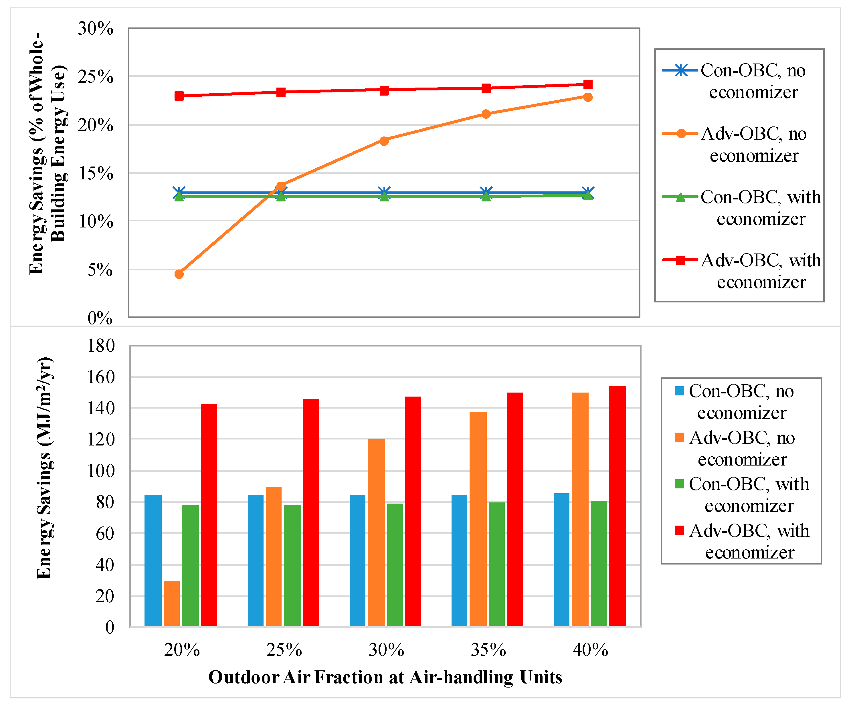
• Relative to the baseline not using occupancy-based controls, the conventional OBC has about 13% whole-building energy savings (around 80 MJ/m²/yr), which barely changes with the OA fraction and economizer settings (lines or bars in green and blue in Figure 7). This happens because the OA fraction does not play a role in the conventional OBC strategy. When a conference room or all private offices in a zone are completely vacant, the corresponding terminal box’s minimum airflow rate is reset to zero. In other words, the setting of a terminal box’s minimum airflow rate depends only on the occupancy schedule, not on the OA fraction.
• The impact of AHU OA fraction on energy savings from the advanced OBC depends on whether an economizer is used. The case of advanced OBC with economizer control has its percentage energy savings (relative to the whole-building energy use) changed marginally from 23% to 24% (the red line in Figure 7) when the OA fraction is increased from 20% to 40%. In contrast, the case of advanced OBC without economizer control has its percentage energy savings changed from about 5% to 23% (the orange line in Figure 7) when the OA fraction is increased from 20% to 40%.
• Under the advanced OBC, the differences of percentage energy savings between the cases with economizer controls and the corresponding cases without economizer controls diminishes as the OA fraction increases. For a single-duct VAV system, the OA fraction in the air stream supplied to the terminal boxes is the same as the AHU OA fraction. As the AHU OA fraction increases, the total airflow rate for each VAV terminal box necessary to meet the ventilation requirement decreases (see Equation (6)). However, beyond a certain limit, the ventilation-driven terminal box airflow rate may become less than the thermal-load-driven airflow rate. Whenever the terminal box airflow rate is driven by the zone thermal loads instead of ventilation, the OA fraction no longer affects the terminal box’s airflow rate and the reheating energy consumption.
• Except for the case with 20% OA fraction and no economizer control, all advanced OBC cases have higher percentage energy savings than the corresponding cases of conventional OBC. The exceptional case of not having energy savings from the advanced OBC can be explained as follows. The conventional OBC strategy resets the terminal box’s minimum airflow rate to zero when all spaces (i.e., conference rooms and private offices) served by the terminal box are unoccupied, which implies that no ventilation is provided at all if an unoccupied zone is in the deadband mode. Meanwhile, the minimum airflow rate is not reset from the baseline if any space served by the terminal box is occupied. The conventional OBC does not guarantee the provision of sufficient ventilation to spaces per ASHRAE Standard 62.1. On the contrary, the advanced OBC always meets the ventilation standard in principle. Thus, in comparison with the conventional OBC and the baseline, the energy savings achieved by advanced OBC has balanced out the impact of improved ventilation.

To support the claim of improved ventilation from the advanced OBC, further analysis of zone ventilation is performed. For the three-floor medium office building simulated in this study, zones on the top floor have the highest thermal loads because of their roof exposure. For two zones with the same design ventilation airflow rate, the one with a larger thermal load requires a higher airflow rate, which means more OA is supplied to the zone with a larger thermal load. Therefore, using the zones on the top floor is a reasonable choice when comparing the advanced OBC against the original baseline and the conventional OBC with respect to their capability to satisfy the ventilation requirement. Figure 8 shows the distribution of annual operation hours according to the deviation of actual provided OA from the OA requirement calculated from Equation (5). The green bar indicates that percentage of annual operation hours when the actual OA provided to the zone meets the requirement, while the blue, orange, and red bars indicate the actual OA is below the ventilation requirement by less than 10%, between 10% and 20%, and greater than 20%, respectively. Figure 8 shows that the advanced OBC meets the ventilation requirement for all zones. Both the baseline and the conventional OBC have many hours not meeting the ventilation requirement, which is especially the case for perimeter ZN 1 (conference room), perimeter ZN 3 (north orientation), and the core zone.

7.3. Impact of Climates

In this section, savings results are presented for two additional locations Miami, FL, with a hot and humid climate and Chicago, IL, with a cold climate. Figure 9 shows the results, from which the following observations can be made:

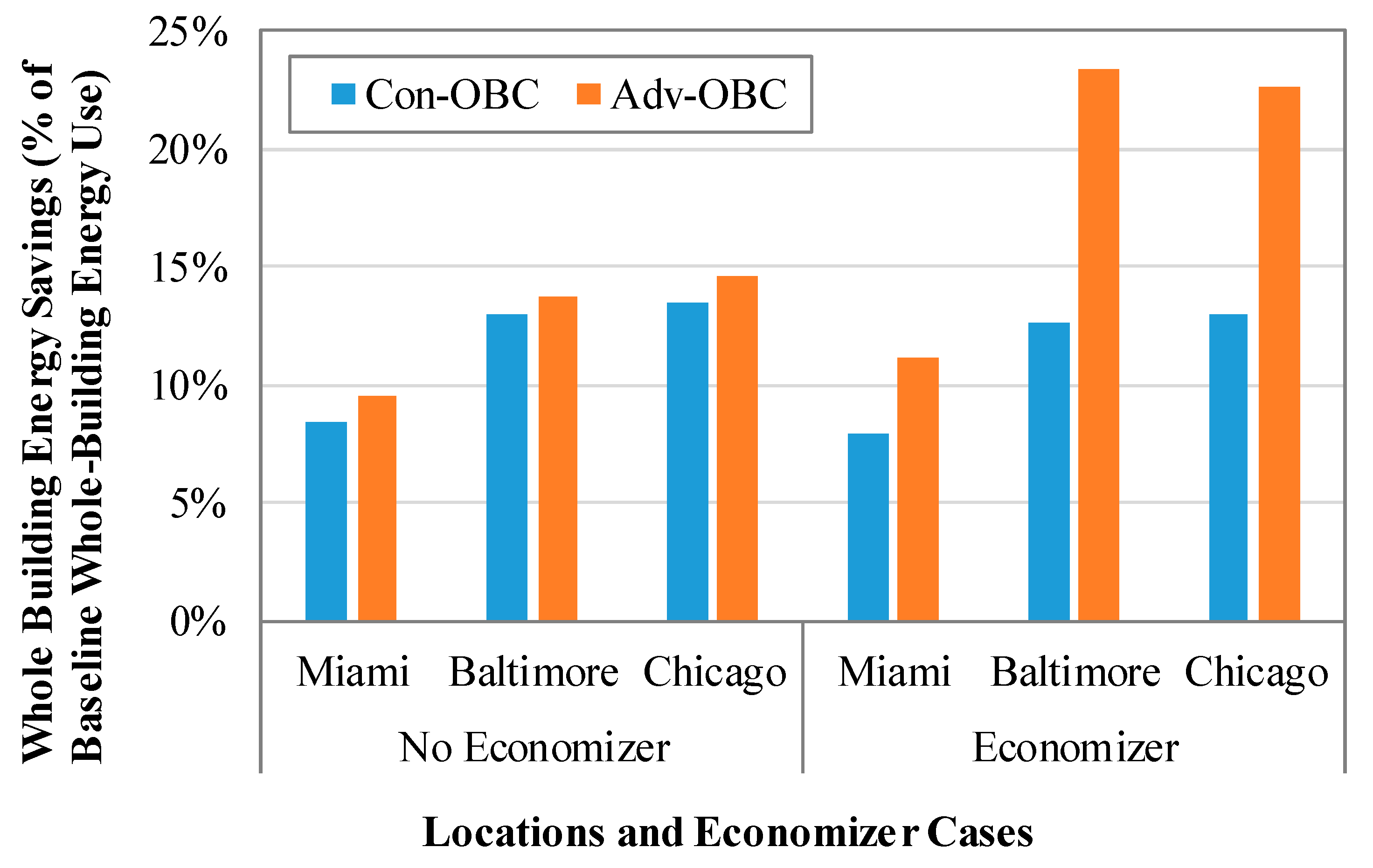
• For each location, the energy savings are nearly equal for the two OBC strategies if the AHUs are not equipped with economizer controls;
• The energy savings for the advanced OBC are much greater than the energy savings for the conventional OBC if the AHUs have economizer controls;
• Baltimore and Chicago have similar energy savings as percentages of baseline energy use for both OBC cases;
• Compared to Baltimore and Chicago, Miami has the smallest percentage savings relative to its baseline energy use. The underlying reason for this is the combination of the following: (1) Miami has a very small heating load relative to the other two locations, and (2) OBC reduces reheating energy more than the other affected energy uses (see Figure 6).

7.4. Comparison of Results with Previous Relevant Work

It is difficult to make comparisons between studies that differ in control strategies, values of parameters, baseline models, and locations/climates. This section positions the findings of this paper in the context of similar work performed previously, without the intention to use the comparisons for rigorous verification of our results. Based on the literature in Section 2, we selected two closely related studies and made a high-level comparison in the following.

The simulation by Goyal et al. [23] for a single zone for three typical days in Gainesville, FL, showed the advanced OBC saved about 48% of HVAC energy use based on an AHU OA fraction of 60%. Our simulation results show savings of about 9.5% of whole-building annual energy use in Miami for the case of 25% OA fraction without an AHU economizer. Because HVAC accounts for about 40% of the whole-building energy use in Miami in the baseline model, the savings of 9.5% of whole-building energy use is equivalent to savings of 24% expressed as a percentage of HVAC energy use. Major factors that likely caused the difference in results include: (1) Goyal et al. used a much higher OA fraction than ours (60% vs. 25%); (2) for the baseline model, they had a fixed occupancy profile (08:00 to 12:00 and 13:00 to 17:00), which had fewer occupied hours than the work presented in this paper; (3) they modeled a single zone while we considered shared spaces; and (4) Goyal et al. simulated three days while the current work simulated a year.

The simulation by Zhang et al. [25] considered a large office building in 16 U.S. climate zones. Because the economizer was used in their work, the results for the case of 25% OA with an AHU economizer from our work is compared with theirs. They found the energy savings as a percentage of whole-building energy use for conventional OBC of 2.6% for Miami, 6.4% for Baltimore, and 6.2% for Chicago while our results are 8.0%, 12.6%, and 13% for the same three locations, respectively. For the advanced OBC, Zhang et al. obtained savings of 5%, 20%, and 19% as percentages of whole-building energy use, respectively, for Miami, Baltimore, and Chicago, while we obtained 11%, 23%, and 23% for the same three locations, respectively. Differences in the results are likely attributable to the following. First, the large office building floor plan used by Zhang et al. has a higher percentage of core zone than the medium office building simulated in the present work (71% vs. 59%). As Table 3 shows, among the three space types, open-plan offices (used for the core zones in both studies) have the fewest OBC control improvements compared to the baseline, thus the smaller savings as percentages of whole-building energy use for the large office building studied by Zhang et al. Secondly, the present study implements many changes in the approaches for modeling occupancy, OA fraction, and terminal boxes, as discussed near the end of Section 2.

8. Conclusions

VAV systems are widely used in commercial buildings. A fixed minimum airflow rate for ventilation (30% or more of the terminal design airflow rate), which is typically used in terminal box control sequences, does not account for occupancy. However, office occupancy varies during a workday, from day to day, and over the longer term. If the minimum airflow rate is higher than required to meet the zone load (including both the thermal load and the ventilation load), unnecessary reheating of the cooled air from the air handler will occur, and the AHU will consume more fan power than necessary. The resulting over-ventilation, during times when the space has less than maximum occupancy or is fully unoccupied, wastes significant fan power, resulting in energy waste and even causing discomfort for occupants in some spaces (e.g., conference rooms) from overcooling. Occupancy-based terminal box controls have the potential to provide large energy savings and improve thermal comfort and indoor air quality by resetting terminal minimum airflow rates based on sensed occupancy. In addition, the sensed occupancy can be used for lighting control and thermostat setpoint reset.

Many commercial products are available on the market to detect whether a space is occupied or not. Advanced occupancy sensors for people counting are also available, although they are expensive currently; however, the U.S. Department of Energy’s Advanced Research Project Agency-Energy is currently funding research and development to decrease the cost and improve the performance of occupant counting sensor technology [40]. With these two different kinds of occupancy sensors, it is important to devise occupancy-based control (OBC) strategies and estimate their potential benefits. A model that represents a currently standing medium office building constructed in the late 1980s was used in the OBC research presented in this paper. Major conclusions from this work include:

• The conventional OBC can save whole-building energy use in the range from 8.0% in Miami (hot climate) to 13% in Chicago (cold climate), while the advanced OBC can save energy by 11.2% to 23.4%;
• For two of the three locations investigated, Baltimore and Chicago, more than half of the saved energy comes from the reduction of reheating energy. OBC also saves energy on cooling, lighting, and ventilation;
• AHU OA fraction is an important parameter that affects the potential energy savings from the advanced OBC strategy. In this regard, whether the AHU has economizer controls and the minimum OA fraction used for the AHU supply air may be critical to determining which occupancy sensor type is most cost-effective for retrofits of existing building for energy savings;
• Energy savings from the conventional OBC do not change with the AHU OA fraction because the OA fraction is not used to determine the minimum terminal airflow rate;
• In addition to energy savings, advanced OBC satisfies the zone ventilation during all occupied hours over the whole year. However, if the terminal box design is based on thermal load only, neither conventional OBC nor the baseline guarantees the satisfaction of the zone ventilation requirement.

In this paper, the primary focus of advanced OBC is on terminal box controls. According to the number of people present in a zone, the minimum airflow rate is changed to just meet, but not exceed, the ventilation need. As shown by the simulation results, the AHU OA fraction has a significant impact on the energy savings of advanced OBC. Hence, it will be worthwhile for a future study to combine the terminal box airflow rate control and the AHU OA flow control for the purpose of system optimization. In addition, even though EnergyPlus is state-of-the-art building performance simulation software that has gone comprehensive testing of its component models, the simulation results for whole-building annual energy savings from the application of OBC need to be validated through field studies.

References

1. Energy Information Administration (EIA). Commercial Buildings Energy Consumption Survey 2012—Microdata; U.S. Department of Energy: Washington, DC, USA, 2016. Available online: https://www.eia.gov/consumption/commercial/data/2012/ (accessed on 5 April 2020).
2. Winiarski, D.W.; Halverson, M.A.; Butzbaugh, J.B.; Cooke, A.L.; Bandyopadhyay, G.K.; Elliott, D.B. Analysis for Building Envelopes and Mechanical Systems Using 2012 CBECS Data; Office of Scientific and Technical Information (OSTI): Richland, WA, USA, 2018; p. 26949.
3. Liu, G.; Brambley, M.R. Occupancy based control strategy for variable-air-volume (VAV) terminal box systems. ASHRAE Trans. 2011, 117, 244–252. [Google Scholar]
4. ASHRAE. ASHRAE Handbook—HVAC Systems and Equipment; American Society of Heating, Refrigerating and Air-Conditioning Engineers Inc.: Atlanta, GA, USA, 2016. [Google Scholar]
5. Taylor, S.T.; Stein, J.; Paliaga, G.; Cheng, H.C. Dual maximum VAV box control logic. ASHRAE J. 2012, 54, 16–24. [Google Scholar]
6. Stein, J.; Zhou, A.; Cheng, H. Advanced Variable Air Volume System Design Guide. 2007. Available online: http://www.taylor-engineering.com/Websites/taylorengineering/images/guides/EDR_VAV_Guide.pdf (accessed on 5 April 2020).
7. Cho, Y.-H.; Liu, M. Minimum airflow reset of single duct VAV terminal boxes. Build. Environ. 2009, 44, 1876–1885. [Google Scholar] [CrossRef]
8. Stein, J. Specifying VAV boxes. HPAC Eng. 2005, 77, 40–44. [Google Scholar]
9. Zhu, Y.; Batten, T.; Noboa, H.; Claridge, D.E.; Turner, W.D.; Liu, M.; Zhou, J.; Cameron, C.; Keeble, D.; Hirchak, R. Optimization Control Strategies for HVAC Terminal Boxes. In Proceedings of the 12th Symposium on Improving Building Systems in Hot and Humid Climates, San Antonio, TX, USA, 15–17 May 2000. [Google Scholar]
10. Taylor, S.T.; Stein, J. Sizing VAV boxes. ASHARE J. 2004, 46, 30–35. [Google Scholar]
11. ASHRAE. ANSI/ASHRAE Standard 62-2019: Ventilation for Acceptable Indoor Air Quality; American Society of Heating, Refrigerating and Air-Conditioning Engineers Inc.: Atlanta, GA, USA, 2019. [Google Scholar]
12. Labeodan, T.; Zeiler, W.; Boxem, G.; Zhao, Y. Occupancy measurement in commercial office buildings for demand-driven control applications—A survey and detection system evaluation. Energy Build. 2015, 93, 303–314. [Google Scholar] [CrossRef] [Green Version]
13. Dougan, D.S.; Damiano, L. CO2-based demand control ventilation: Do risks outweigh potential rewards. ASHRAE J. 2004, 46, 47–53. [Google Scholar]
14. Emmerich, S.J.; Persily, A.K. State-of-the-Art Review of CO2 Demand Controlled Ventilation Technology and Application; NIST: Gaithersburg, MD, USA, 2001.
15. Schell, M.; Inthout, D. Demand control ventilation using CO2. ASHRAE J. 2001, 43, 1–6. [Google Scholar]
16. Taylor, S.T. CO2-based DCV using 62.1-2004. ASHRAE J. 2006, 48, 67–75. [Google Scholar]
17. Lu, T.; Lu, X.; Viljanen, M. A novel and dynamic demand-controlled ventilation strategy for CO2 control and energy saving in buildings. Energy Build. 2011, 43, 2499–2508. [Google Scholar] [CrossRef]
18. Nassif, N.; Kajl, S.; Sabourin, R. Ventilation Control Strategy Using the Supply CO2 Concentration Setpoint. HVAC R Res. 2005, 11, 239–262. [Google Scholar] [CrossRef] [Green Version]
19. Murphy, J. CO2-based demand-controlled ventilation with ASHRAE Standard 62.1. Eng. Newsl. 2005, 34, 5. [Google Scholar]
20. Lin, X.; Lau, J. Demand controlled ventilation for multiple zone HVAC systems: CO2-based dynamic reset (RP 1547). HVAC R Res. 2014, 20, 875–888. [Google Scholar] [CrossRef]
21. Kang, S.-H.; Kim, H.-J.; Cho, Y.-H. A study on the control method of single duct VAV terminal unit through the determination of proper minimum air flow. Energy Build. 2014, 69, 464–472. [Google Scholar] [CrossRef]
22. Balaji, B.; Xu, J.; Nwokafor, A.; Gupta, R.; Agarwal, Y. Sentinel: Occupancy based HVAC actuation using existing WiFi infrastructure within commercial buildings. In Proceedings of the 11th ACM Conference on Embedded Networked Sensor Systems, Rome, Italy, 11–13 November 2013. [Google Scholar]
23. Goyal, S.; Ingley, H.A.; Barooah, P. Occupancy-based zone-climate control for energy-efficient buildings: Complexity vs. performance. Appl. Energy 2013, 106, 209–221. [Google Scholar] [CrossRef]
24. Brooks, J.; Goyal, S.; Subramany, R.; Lin, Y.; Liao, C.; Middelkoop, T.; Ingley, H.; Arpan, L.; Barooah, P.; Arpan, P. Experimental evaluation of occupancy-based energy-efficient climate control of VAV terminal units. Sci. Technol. Built Environ. 2015, 21, 469–480. [Google Scholar] [CrossRef]
25. Zhang, J.; Lutes, R.G.; Liu, G.; Brambley, M.R. Energy Savings for Occupancy-Based Control (OBC) of Variable-Air-Volume (VAV) Systems. In Energy Savings for Occupancy-Based Control (OBC) of Variable-Air-Volume (VAV) Systems; Pacific Northwest National Laboratory: Richland, WA, USA, 2013. [Google Scholar]
26. Oldewurtel, F.; Sturzenegger, D.; Morari, M. Importance of occupancy information for building climate control. Appl. Energy 2013, 101, 521–532. [Google Scholar] [CrossRef]
27. Department of Energy (DOE). EnergyPlus Software, Version 8.0. 2015. Available online: https://energyplus.net/ (accessed on 1 June 2020).
28. Deru, M.; Field, K.; Studer, D.; Benne, K.; Griffith, B.; Torcellini, P.; Liu, B.; Halverson, M.; Winiarski, D.; Rosenberg, M.; et al. U.S. Department of Energy Commercial Reference Building Models of the National Building Stock; NREL: Golden, CO, USA, 2011.
29. Persily, A.; Gorfain, J.; Brunner, G. Ventilation design and performance in U.S. office buildings. ASHRAE J. 2005, 47, 30–35. [Google Scholar]
30. Page, J.; Robinson, D.; Morel, N.; Scartezzini, J.-L. A generalised stochastic model for the simulation of occupant presence. Energy Build. 2008, 40, 83–98. [Google Scholar] [CrossRef]
31. ASHRAE. ANSI/ASHRAE/IESNA Standard 90.1-2004: Energy Standard for Buildings Except Low-Rise Residential Buildings; American Society of Heating, Refrigerating and Air-Conditioning Engineers, Inc.: Atlanta, GA, USA, 2004. [Google Scholar]
32. Yu, Y.; Xu, K.; Cho, Y.; Liu, M. A smart logic for conference room terminal box of single duct VAV system. In Proceedings of the 7th International Conference for Enhanced Building Operations 2007, San Francisco, CA, USA, 1–2 November 2007. [Google Scholar]
33. ASHRAE. ANSI/ASHRAE Standard 62-2004: Ventilation for Acceptable Indoor Air Quality; American Society of Heating, Refrigerating and Air-Conditioning Engineers Inc.: Atlanta, GA, USA, 2004. [Google Scholar]
34. Pang, X.; Piette, M.A.; Zhou, N. Characterizing variations in variable air volume system controls. Energy Build. 2017, 135, 166–175. [Google Scholar] [CrossRef] [Green Version]
35. Wang, D.; Federspiel, C.C.; Rubinstein, F. Modeling occupancy in single person offices. Energy Build. 2005, 37, 121–126. [Google Scholar] [CrossRef]
36. Hart, R. RE: Impact of Recent ASHRAE 62.1 Standard Committee Interpretations on 2013 Title 24 Code Ventilation Proposals; California Energy Commission—Docket 12-BSTD-1, February 2012; PECI, Inc.: Portland, OR, USA, 2012. Available online: https://efiling.energy.ca.gov/Lists/DocketLog.aspx?docketnumber=12-BSTD-01 (accessed on 21 February 2020).
37. Gunay, H.B.; O’Brien, W.; Beausoleil-Morrison, I. Implementation and comparison of existing occupant behaviour models in EnergyPlus. J. Build. Perform. Simul. 2015, 9, 1–46. [Google Scholar] [CrossRef]
38. Von Neida, B.; Maniccia, D.; Tweed, A.; Manicria, D. An Analysis of the Energy and Cost Savings Potential of Occupancy Sensors for Commercial Lighting Systems. J. Illum. Eng. Soc. 2001, 30, 111–125. [Google Scholar] [CrossRef]
39. Department of Energy (DOE). Weather Data Sources. 2020. Available online: https://energyplus.net/weather/sources#TMY3 (accessed on 28 June 2020).
40. ARPA-E. SENSOR, Saving Energy Nationwide in Structures with Occupancy Recognition. U.S. Department of Energy, Advanced Research Projects Agency—Energy. 2017. Available online: https://arpa-e.energy.gov/?q=arpa-e-programs/sensor (accessed on 21 February 2020).
Figure 1. Schematic of research methodology.
Energies 13 03756 g001
Figure 2. Modeled medium office building: (a) Floor plan and zoning; (b) isometric view.
Energies 13 03756 g002
Figure 3. The probability of occupant presence in offices.
Energies 13 03756 g003
Figure 4. The probability of occupant presence in conference rooms.
Energies 13 03756 g004
Figure 5. Interior lighting profiles used in the baseline model for both offices and conference rooms.
Energies 13 03756 g005
Figure 6. Annual energy savings of affected end uses from occupancy-based control in MJ/m2-yr and percentage of baseline whole-building energy use for the medium office building in Baltimore, MD.
Energies 13 03756 g006
Figure 7. Energy savings relative to baseline energy use from occupancy-based controls for the medium office building in Baltimore, MD, at different settings of the minimum outdoor air fraction during the time of AHU running.
Energies 13 03756 g007
Figure 8. The distribution of annual operation hours according to the deviation of actual provided outdoor air (OA) from the OA requirement of the five zones on the top floor of the medium office building in Baltimore, MD.
Energies 13 03756 g008
Figure 9. Energy savings from occupancy-based controls for the medium office building in three different climates.
Energies 13 03756 g009