Article

Robustness of Short-Term Wind Power Forecasting against False Data Injection Attacks

Shaanxi Key Laboratory of Smart Grid, School of Electrical Engineering, Xi’an Jiaotong University, Xi’an 710049, China
*
Author to whom correspondence should be addressed.
Energies 2020, 13(15), 3780; https://doi.org/10.3390/en13153780
Submission received: 8 July 2020 / Revised: 20 July 2020 / Accepted: 22 July 2020 / Published: 23 July 2020
(This article belongs to the Section A3: Wind, Wave and Tidal Energy)

Abstract

:
The accuracy of wind power forecasting depends a great deal on the data quality, which is so susceptible to cybersecurity attacks. In this paper, we study the cybersecurity issue of short-term wind power forecasting. We present one class of data attacks, called false data injection attacks, against wind power deterministic and probabilistic forecasting. We show that any malicious data can be injected to historical data without being discovered by one of the commonly-used anomaly detection techniques. Moreover, we testify that attackers can launch such data attacks even with limited resources. To study the impact of data attacks on the forecasting accuracy, we establish the framework of simulating false data injection attacks using the Monte Carlo method. Then, the robustness of six representative wind power forecasting models is tested. Numerical results on real-world data demonstrate that the support vector machine and k-nearest neighbors combined with kernel density estimator are the most robust deterministic and probabilistic forecasting ones among six representative models, respectively. Nevertheless, none of them can issue accurate forecasts under very strong false data attacks. This presents a serious challenge to the community of wind power forecasting. The challenge is to study robust wind power forecasting models dealing with false data attacks.

1. Introduction

Traditionally, the power system is seen as a physical system to generate, transmit, and deliver the electricity. With the development of information and communication technology, the cyber system is now playing a more and more important role for situation awareness and security control in the modern power system [1]. However, the malicious cyberattack targeting the Ukrainian electricity grid in 2015 [2] let governments realize for the first time that the failure of the cyber system could also damage the physical power system. Since then, more and more attention has been paid to the cybersecurity issue of the power system [3].
Energy forecasting (including load, electricity price, and renewable generation forecasting) is also a very important component of cyber-physical power systems, especially for modern power systems with high penetration of renewable energy. It is well-known that power system operations heavily rely on very accurate forecasts, such as load and renewable energy forecasting [4,5,6]. Unfortunately, as pointed out by Luo et al. [7] for the first time, energy forecasting is very vulnerable to false data attacks (one type of cyberattacks). This is because the input data quality directly affects the forecast accuracy. Through false data attacks, hackers can inject malicious data into the historical (input) data and then deteriorate the forecast quality significantly. Thus, the cybersecurity issue of energy forecasting is now an important emerging problem for power system research.
To deal with the aforementioned challenge, some pioneering research has been undertaken to first study the cybersecurity of load forecasting [7,8,9,10,11,12,13]. The influence of false data attacks on the accuracy of load forecasting was first studied by Luo et al. [7]. The robustness of four representative load forecasting models was then tested and compared under various false data attacks. To detect false data attacks and identify the injected malicious data, anomaly detection tools based on dynamic regression [8], machine learning [10], and descriptive analytics [11] have been already proposed for protecting load forecasting. Finally, some robust approaches of load forecasting were developed in [9,12] and numerical experiments demonstrate that they can provide accurate load forecasts even under false data attacks.
Up to now, most of research focuses on the cybersecurity of load forecasting. However, little work has been done on the robustness of renewable generation forecasting, especially wind power forecasting, under false data attacks. Wind power forecasting [14,15] has found its wide applications in the power industry, because the power industry requires accurate wind power forecasting to reduce the impacts of wind power volatility on power system operation [4] and electricity market transaction [5]. In terms of the forecast horizon, wind power forecasting could be divided into three groups, i.e., very short-term forecasts (from minutes to hours) [16], short-term forecasts (up to 2 days) [17], and medium-term forecasts (up to 7 days) [18]. Forecast errors generally increase with the forecast horizon increasing [19]. Physical and statistical methods are two overall families of forecasting models for wind power. Physical methods rely on meso-scale atmospheric models but require very high computing power [20]. Statistical methods directly map the relationship between wind power data and meteorology data [21]. Representative statistical methods include autoregressive integrated moving average models (ARIMA) [22,23], artificial neural networks (ANN) [24,25], support vector machines (SVM) [26,27]. On the other hand, hybrid or ensemble methods combining the benefits of different forecasting models show better performance than using only a single method [28].
As mentioned earlier, false data attacks are expected to deteriorate the accuracy of wind power forecasting. Inaccurate forecasting will induce poor or even wrong decision making of power system operation in various aspects, such as reserve requirement determination [6]. Thus, studying the robustness of wind power forecasting under cyberattacks becomes an urgent requirement for ensuring power system reliability, security, and resilience. Furthermore, previous research on the cybersecurity of load forecasting [7] simulated false data attacks by randomly injecting some multipliers that follow an assumed distribution. However, one major drawback of [7] is that it did not apply any anomaly detection techniques to preprocess the malicious data injected by false data attacks, which is not true in reality.
On the other hand, in recent years, wind power probabilistic forecasting [29,30,31,32,33,34,35] has gained increasing attention, driven by the strong requirement to quantify the uncertainty of wind power output. Parametric and non-parametric methods are two different families. For examples, quantile regression [29], kernel density estimator [30,31,35], and the hybrid method [33] have been studied in recent years. Nevertheless, none has extended the cybersecurity concern from the traditional deterministic (point) to probabilistic forecasting up to now. Thus, it would be very valuable to further study their cybersecurity issues.
In this paper, we study the effect of false data attacks on the accuracy of short-term wind power forecasting (including deterministic and probabilistic ones). Main contributions of this paper are summarized as follows:
  • A false data injection attack approach against wind power forecasting is first developed where the attacker can inject any amount of malicious data into wind data without being detected by the least-squares-based anomaly detection tool.
  • The Monte Carlo simulation framework is established to simulate false data injection attacks on wind power data and meteorological data. The Monte Carlo simulation framework can be utilized to evaluate the robustness of any wind power forecasting models.
  • It benchmarks the accuracy of six representative wind power forecasting approaches (including three deterministic ones and three probabilistic ones) under different attack intensities and different attack targets (including wind power data and meteorological data).
To the best of our knowledge, this is the first effort to study the cybersecurity issue of wind power forecasting and systematically evaluate the robustness of some wind power forecasting models under false data attacks.
The remainder of this paper is organized as follows. Section 1 gives a brief introduction about the architecture of the wind energy management system and also proposes potential false data attack scenarios. Section 3 presents the principles of false data injection attacks. Section 4 reviews six representative short-term wind power forecasting models. Section 5 provides a robustness assessment framework of the wind power forecasting approach. Section 6 gives the data and all model setups. Section 7 shows numerical results of the comparative study. Finally, this paper is concluded in Section 8.

2. Cyber Attack Scenarios on Wind Energy Management System

The information and communication technology (ICT) is of crucial importance for wind farm management [36]. The supervisory control and data acquisition (SCADA) system and energy management system (EMS) are two typical ICT services for monitoring and operating wind farms [37]. In this section, we review the architecture of the wind farm SCADA/EMS system. After that, the cyber security for the wind farm SCADA/EMS system is studied. Credible false data attack scenarios against the wind farm SCADA/EMS system are developed consequently.

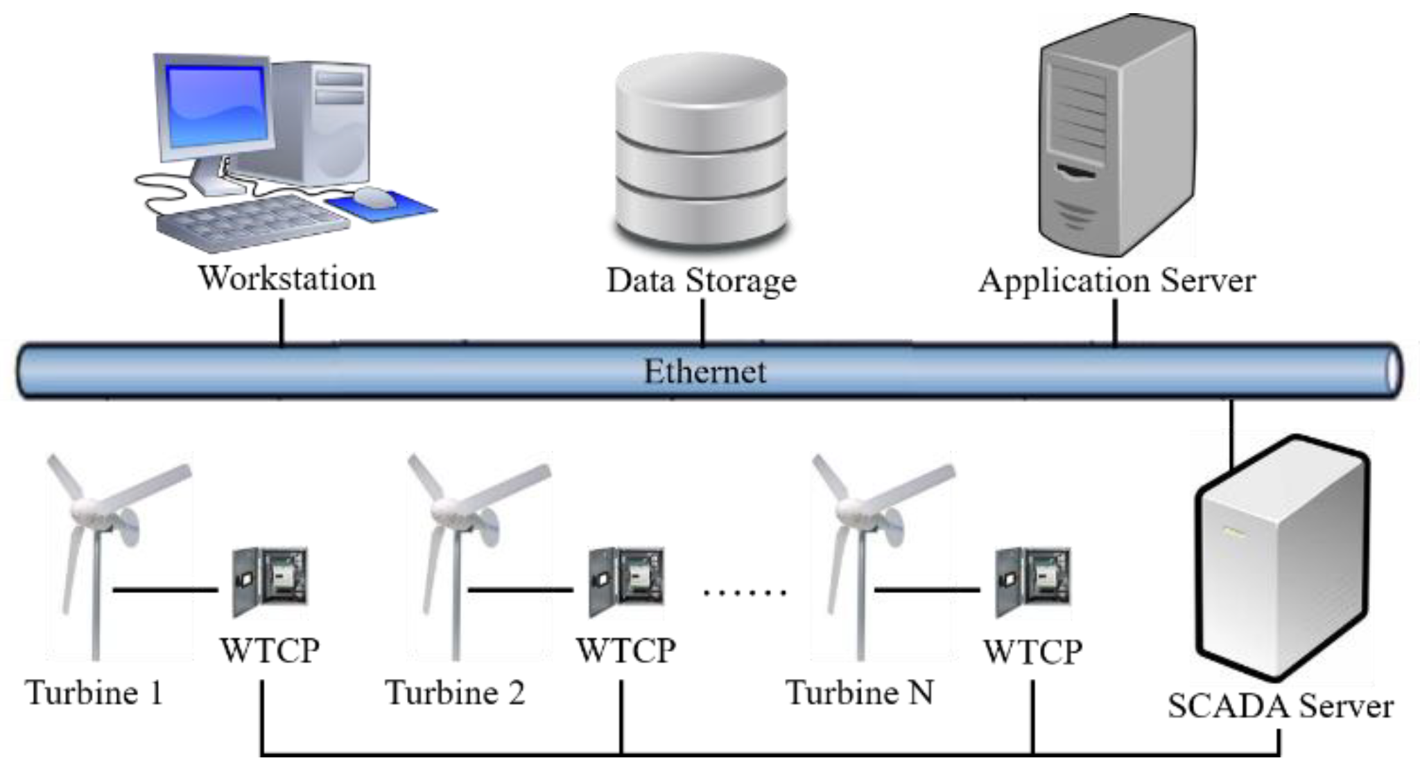
2.1. Architecture of Wind Farm SCADA/EMS System

The typical architecture of the wind farm SCADA/EMS system was introduced in Yan et al. [38] and Zhang et al. [39] In this section, we first review the architecture of the SCADA system installed in every wind farm. Then, we review the EMS architecture of integrating and managing multiple wind farms.
Figure 1 shows the representative architecture of the SCADA system installed in every wind farm. This system is used to monitor and operate all wind turbines in the farm. SCADA systems have the ability to communicate with any devices in the farm. Wind turbine is equipped with a control panel, known as the wind turbine control panel (WTCP). In the control room, all data received from meters or outside (such as meteorological data) are stored in the database and transmitted to the application server. Wind farm operators can monitor the status of all wind turbines through the workstation.
On the other hand, some wind power companies run multiple wind farms in different locations. Thus, they need an EMS system to integrate and manage multiple wind farms. Figure 2 shows the representative architecture of the EMS system. All wind farms are integrated into the control center via a control wide area network (WAN). Fiber optics are usually chosen as communication infrastructures to build this control WAN. In this case, the control room in each farm might not be staffed. In the control center, there are several operator consoles to display the information received from all SCADA servers. All data are stored in the historian database.
Wind power forecasting tools are usually deployed in the application server of the SCADA or EMS system. If this tool is run in the SCADA system, it only provides the forecasting service for the target wind farm. However, if this tool is deployed in the EMS system, it can provide the forecasting service for all wind farms of one company. Data in the application server or data storage are utilized to train wind power forecasting models and issue the forecasting result.

2.2. Credible False Data Attack Scenarios

Vulnerabilities of the wind farm SCADA/EMS system are identified in this subsection. Then, multiple credible false data attack scenarios against the wind farm SCADA/EMS system are developed consequently [40,41].

2.2.1. Scenario I: Attack on WTCP

The WTCP is mainly used by maintenance staff to get the operating status and data of wind turbines [38]. The WTCP is usually installed on the tower base and thus it is accessible for attackers. Although the WTCP is usually authorized by a pin, the attacker can still crack the pin by the brute force searching [38] or chemical combination attack [42]. After that, the attacker is able to connect intrusion devices with the WTCP. Malicious data injected into the WTCP would be sent to the SCADA/EMS system, impacting the deployed wind power forecasting service.

2.2.2. Scenario II: Attack on Optical Fiber Cables

Optical fiber cables are usually used as communication links in the SCADA/EMS system [38]. The communication medium of optical fiber is glass or plastic allowing light propagations. Optical fibers can be attacked by advanced tapping methods without being detected [43]. The attacker is able to inject additional light and deduce the underlying signal by installing taps on optical fiber cables. Since the attacker can easily get physical access to fiber cables, this attack presents a very high risk for data integrity in the SCADA/EMS system. Thus, attacks on fiber cables have great damage on wind power forecasting accuracy.

2.2.3. Scenario III: Attack on SCADA/EMS Servers

Servers are used to communicate, store data, and deploy applications in the SCADA/EMS system. However, servers could be impacted by internal attacks [38]. For example, a corrupted but authorized user has physical access to all servers, and then this user can inject malicious data into the historical database. On the other hand, servers can be attacked by infected portable storage devices [38]. Malwares, such as spyware and Stuxnet, are introduced into servers. Then, infected servers will be controlled by attackers and inject malicious data into the historical database.

3. False Data Injection Attack against Wind Power Forecasting

In this section, we present one data attack mode, called false data injection attacks, against short-term wind power forecasting. First, we introduce one of the anomaly detection techniques commonly used in data analysis, which can also be applied to data pre-processing in wind power forecasting. Then, the false data injection attack approach is developed, demonstrating that the attacker can inject any amount of malicious data which may damage wind power forecasting without being detected by the anomaly detection technique. Note that the anomaly detection technique and the false data injection attack approach are both generic, not limited to short-term wind power forecasting. Finally, how to implement such a false data attack on wind power data and meteorological data is presented, respectively.

3.1. Least-Squares-Based Anomaly Detection Technique

From the perspective of data analysis, outliers are associated with abnormal observations as they are supposed to be deviations from normal behavior. In wind power forecasting, outliers can be caused by several reasons, such as measurement errors. Outliers seriously affect the accuracy of wind power forecasting. So, some anomaly detection techniques have been proposed to detect and remove outliers from the original dataset.
The three sigma method was first proposed in [44] to reject outliers in wind power time series data. The abnormal data greater than three times standard deviations from wind power curves were identified as outliers. This idea was then further developed in [45] to consider probabilistic wind power curves. In addition to data-driven methods [44,45], image-driven methods based on wind power curve images were proposed in [46] to identify and clean the abnormal data of wind turbine. Spatial correlation of multiple adjacent wind farms was exploited in [47] to detect and recovery the outliers of one wind farm. The density-based spatial clustering method was proposed in [48] to eliminate the outliers caused by wind curtailment.
The most commonly-used anomaly detection techniques by the power industry are based on regression models [8,49,50,51,52]. The main idea of regression-based anomaly detection methods is to first backcast the data using regression methods and then compare the fitted values with the original ones. If the deviation is larger than a given threshold, the corresponding observation is detected as the outlier. Up to now, different regression methods, such as linear regression [51,52], dynamic regression [8], and non-parametric regression [49,50], have been proposed for different anomaly detection applications.
In this paper, we introduce one of the regression-based anomaly detection techniques commonly used by the power industry. This is referred to as the outlier detection technique based on least squares. For any time series forecasting problems, the original dataset is generally made up of two parts, i.e., input variables x t = ( x t ( 1 ) , x t ( 2 ) , , x t ( n ) ) T n and the output variable y t . n is the number of input variables. The pair ( x t , y t ) is called the t -th example. The original dataset is a list of m examples, i.e., { ( x t , y t ) ; t = 1 , 2 , , m } .
Using least squares regression, the output variable y is approximated by a linear function of input variables x n :
y = θ T x   ,
where θ n is an n -dimensional parameter. Given the original dataset, the parameter θ is estimated by minimizing the least-squares cost function, which can be formalized as follows:
argmin θ 1 2 t = 1 m ( θ T x t y t ) 2 .
The above optimization problem (2) can be rewritten as a matrix form. First, we define the design matrix X m × n as a m -by- n stacked matrix. X contains all examples’ input variables x t in its rows. In the same way, we define the design vector y m containing all examples’ output variable y t :
X = [ ( x 1 ) T ( x 2 ) T ( x m ) T ] ,   y = [ y 1 y 2 y m ] .
Then, we can easily verify that the problem (2) is equivalent to the following problem:
argmin θ 1 2 ( X θ y ) T ( X θ y ) .
The solution of θ for the above optimization problem (4) is given in the closed form as follows:
θ ^ = ( X T X ) 1 X T y .
Substituting θ ^ for θ in (1), we can then obtain the estimated value y ^ = X θ ^ . Intuitively, for the original dataset without outliers, its estimated value y ^ is usually close to its observed value y . While for the dataset with outliers, its estimated value is far away from its observed value. Following this idea, the observation residual (i.e., the difference between observed value and estimated value) is defined as follows:
r = y y ^ = y X θ ^ .
Its L 2 -norm y X θ ^ is used to detect whether outliers exist or not. Specifically, given a threshold τ (considering the acceptable level of observation residuals), outliers exist in the original dataset when the L 2 -norm of residuals is larger than τ (i.e., y X θ ^ > τ ). How to choose the proper threshold τ is also very important, but not in the scope of this paper.

3.2. False Data Injection Attack Approach

In this part, we follow the idea of [53] and develop an alternative approach of false data injection attack against wind power forecasting. We also show that such attack mode cannot be detected successfully by the anomaly detection technique introduced in the previous part. Furthermore, we show how to launch the data injection attack if the attacker only has very limited resource. Here, “limited resource” means the resource, such as computing resource, communicating resource, and human resource, which are required by attackers to launch a data injection attack successfully.
It is assumed that the attacker has local information of the design matrix X of the target wind farm using the approaches shown in Section 2.2. Note that this assumption does not require the attacker to know the full knowledge about the design matrix X . Even if the attacker only knows local information of the design matrix X , e.g., some input features, the attacker can still launch the successful false data attack, as indicated by Theorem 1. Actually, for short-term wind power forecasting problems, the design matrix X is usually made up of numerical weather prediction (NWP) and calendar information. Both of them can be publicly accessible. For example, NWP results can be purchased from meteorological agencies or calculated by using computational fluid dynamics.
Then, the attacker can inject malicious data into the original dataset to affect the quality of short-term wind power forecasting. The attacking target is assumed to be the output variable y . Let ε represent the vector of malicious data injected to the original dataset (also known as the attack vector). The attacker can choose any non-zero attack vector ε and then replace the original data y by the malicious data as follows:
y ε = y + ε .
As discussed in the previous part, the least-squares-based anomaly detection technique computes the L 2 -norm of the observation residual and then checks whether outliers exist or not. But, as indicated by Theorem 1 (similar to Theorem 3.1 in [53]), it can be found that such anomaly detection tool cannot detect the false data attack behavior if the attack vector ε is a linear combination of column vectors of the design matrix X . The proof of Theorem 1 can be found in the Appendix A.
Theorem 1.
Given that the original data y can successfully pass the least-squares-based anomaly detection tool, this means that y X θ ^ τ . The malicious data y ε = y + ε can also pass the anomaly detection tool if the attack vector ε is a linear combination of column vectors of the design matrix X , i.e., ε = X δ , where δ n is a non-zero arbitrary vector.
Remark 1.
According to Theorem 1, the attacker can successfully construct an effective attack vector ε , even though the attacker only has local information of the design matrix X . For example, given that the attacker only knows the second and third columns of the design matrix, i.e., X ^ = { x 2 , x 3 } , then the attack vector ε ^ can be constructed as ε ^ = δ 2 x 2 + δ 3 x 3 , where δ 2 and δ 3 are two non-zero arbitrary values.
On the other hand, the attacker may have limited resource to launch the false data injection attack. As a result, the attacker cannot easily utilize ε = X δ as the attack vector because some of original data cannot be accessed by the attacker. For example, due to the limited resource, the attacker may only inject the malicious data into only 40% of original data. For the remaining 60% of original data that cannot be accessed, nothing can be injected into them. Thus, some elements of the attack vector ε would be 0.
Here, we assume that the attacker has access to L elements of the design vector y (e.g., L examples of wind power measurements). Let t l be the index of the l -th element ( l = 1 , 2 , , L ) and let = { t 1 , t 2 , , t L } be the set of indices of all L elements that the attacker can get access to. According to Theorem 1, in order to pass the anomaly detection, the attacker should find an attack vector ε that satisfies two conditions as follows.
  • ε t = 0 for t (the attacker cannot inject errors into elements that cannot be accessed).
  • ε = X δ ( ε is a linear combination of column vectors of X ).
To construct such an attack vector under the limited resource, we first prove that ε = X δ has an equivalent but more straight-forward form [53].
Theorem 2.
ε = X δ if and only if Q ε = 0 , where Q = X ( X T X ) 1 X T I and I m × m is the identity matrix.
The proof of Theorem 2 can be found in the Appendix A. According to Theorem 2, the attacker needs to construct an attack vector ε that satisfies Q ε = 0 and ε t = 0 for t . Let:
Q = ( q 1 , q 2 , , q m ) ,
where q t ( t = 1 , 2 , , m ) is the t -th column vector of Q . Let:
ε = ( 0 , , 0 , ε t 1 , 0 , , 0 , ε t 2 , 0 , , 0 , ε t L , 0 , , 0 ) T ,
where ε t 1 , ε t 2 , …, ε t L are unknown variables. Substituting (8) and (9) into Q ε = 0 , it is easy to verify that:
Q ε = 0 ( q 1 , q 2 , , q m ) ( 0 , , 0 , ε t 1 , 0 , , 0 , ε t 2 , 0 , , 0 , ε t L , 0 , , 0 ) T = 0
( q t 1 , q t 2 , , q t L ) ( ε t 1 , ε t 2 , , ε t L ) T = 0 .
Then, we create a new m -by- L matrix Q ¯ = ( q t 1 , q t 2 , , q t L ) m × L and a new vector ε ¯ = ( ε t 1 , ε t 2 , , ε t L ) L . Substituting Q ¯ and ε ¯ into (10), we obtain that:
Q ε = 0     Q ¯ ε ¯ = 0 .
According to Meyer [54], the solution of the equation Q ¯ ε ¯ = 0 is:
ε ¯ = ( I Q ¯ 1 Q ¯ ) d ,
where Q ¯ 1 is the Matrix 1-inverse of Q ¯ and d is the L -dimensional arbitrary non-zero vector. Using the non-zero solution ε ¯ , the attacker can construct the corresponding attack vector ε by first filling the element of ε ¯ into the corresponding position of ε and then filling 0 into the remaining position of ε .
Thus, under the limited resource, the attacker can still inject the false data into the original data without being discovered by the least-squares-based anomaly detection tool. Such false data injection attack mode can introduce a large error into wind power forecasting and seriously affect the prediction accuracy.

3.3. False Data Attack on Wind Power Data

In this subsection, the attack target is assumed to be wind power data. Such attack can be launched via compromising some meters in the target wind farm or directly hacking servers which store the original dataset, as shown in Section 2.2.
First, the anomaly detection technique based on least squares to identify the outliers in wind power data is presented. The outliers in wind power data are detected by least squares regression on exogenous inputs. To consider the nonlinear relationship between wind power output and wind speed, three regressors are constructed, i.e., linear, quadratic, and cubic regressors. On the other hand, four Fourier regressors are also constructed to model the daily seasonality observed in wind power data. Thus, the nonlinear regression model used to detect the outliers in wind power data can be written as:
y ^ t = θ 1 x t + θ 2 x t 2 + θ 3 x t 3 + θ 4 cos ( 2 π 24 d t ) + θ 5 sin ( 2 π 24 d t ) + θ 6 cos ( 4 π 24 d t ) + θ 7 sin ( 4 π 24 d t ) ,
where x t is the wind speed at time t ( t = 1 , 2 , , m ). d t is the time (24 h) of a day at time t (taking the value of 0, 1, 2, …23). The design matrix X contains all seven regressors in its rows, as shown below:
X = [ x m   x m 2   x m 3   cos ( 2 π 24 d m )   sin ( 2 π 24 d m )   cos ( 4 π 24 d m )   sin ( 4 π 24 d m )               x 1   x 1 2   x 1 3   cos ( 2 π 24 d 1 )   sin ( 2 π 24 d 1 )   cos ( 4 π 24 d 1 )   sin ( 4 π 24 d 1 ) ] .
According to Theorem 1 or Theorem 2, we can construct the attack vector ε injected to wind power data. The attack vector ε would not be detected by least-squares-based anomaly detection techniques if it is a linear combination of column vectors of the design matrix X .

3.4. False Data Attack on Meteorological Data

Meteorological data is of crucial importance for short-term wind power forecasting and is generally obtained from external services. Thus, it is much easier for attackers to inject malicious data into meteorological information and then deteriorate the forecasting quality significantly.
First, the anomaly detection technique based on least squares to identify the outliers in meteorological data is presented. Different from wind power data where its outliers are detected by using exogenous inputs (such as wind speed and direction), meteorological data usually have no exogenous inputs. Hence, the autoregression model is selected to identify the outliers in meteorological data. The term autoregression (AR) indicates that it is a regression of a meteorological variable against itself. The meteorological data are approximated by a linear combination of past values of itself. The AR model of order p for meteorological data can be written as:
x ^ t = θ 1 x t 1 + θ 2 x t 2 + + θ p x t p .
Then, we can calculate the residual between the observed value x t and the estimated value x ^ t by AR models, i.e., r t = x t x ^ t . Given a threshold τ , the outlier exists in meteorological data if the absolute residual | r t | is larger than τ .
According to Theorem 1, we can construct the attack vector ε injected to meteorological data. The attack vector ε would not be detected by the anomaly detection technique based on the aforementioned AR model if it is a linear combination of column vectors of the design matrix X . Here, the design matrix X for AR models contains the lagged meteorological data in its rows, as shown below:
X = [ x m 1 x m 2 x m p           x p   x p 1   x 1   ] ,
where x t represents the meteorological data at time t ( t = 1 , 2 , , m 1 ). Then, the attack vector is constructed according to Theorem 1 or Theorem 2.

4. Wind Power Forecasting Models

In this section, six representative wind power forecasting approaches (including three deterministic ones and three probabilistic ones) are briefly introduced. These approaches have been widely used in power system operation and planning [55,56]. The robustness of these six forecasting approaches would be investigated in our case studies of Section 7.

4.1. Deterministic Forecasting Models

Deterministic (or point) forecasting provides the conditional expectation of wind power output. Three wind power deterministic forecasting models are introduced as follows.

4.1.1. Multiple Nonlinear Regression (MNR)

MLR is one of the widely-used techniques for many forecasting problems. In short-term wind power forecasting, wind power output is treated as the responsible variable y , while wind forecasting from NWP and calendar variables are usually treated as input variables x [4,31]. The generic fitting formula of MLR models is y = θ T x . Given the training dataset, the parameter vector θ can be estimated by minimizing the sum of square errors, as shown in (2). The solution of θ is given in (5).

4.1.2. Artificial Neural Network (ANN)

ANN originates from algorithms that try to mimic the human brain. It has been very widely used in many forecasting problems including wind power forecasts since the 1980s. Its popularity once diminished in the late 1990s. But recently, with the rapid development of deep learning, ANN has regained quite a lot of attention. As a data-driven black-box approach, ANN can approximate the nonlinear relationship between all input variables and wind power output by learning from the training data. ANN-based short-term wind power forecasting was also commercialized and used by many forecasting vendors [24].
In this paper, we use a three-layer feed-forward neural network to provide short-term wind power forecasting [24]. Every input neuron is connected to every hidden neuron. There is only one output neuron representing wind power output. The sigmoid function is chosen as activation functions for hidden and output neurons. This ANN model is trained by the Levenberg–Marquardt backpropagation algorithm. Furthermore, this ANN model has two important hyperparameters, i.e., the number of hidden neurons and the weight decay. Both of them are optimized through k-fold cross validation.

4.1.3. Support Vector Machine (SVM)

SVM approaches first map the original data to a high-dimensional space through a nonlinear transform. Then, we can apply the traditional linear regression in the high-dimensional space, which is equivalent to the nonlinear regression in the low-dimensional space. Quite a lot of papers have reported how to use SVM in short-term wind power forecasting [26].
In this paper, we utilize a specific SVM model called ϵ -SVM for short-term wind power forecasting [26]. For the training dataset { ( x i , y i ) ; i = 1 , 2 , , m } , the ϵ -SVM model tries to obtain the parameter vector θ of the fitting hyperplane y = θ T x . SVM approaches have two important hyperparameters, i.e., γ and ϵ . Their optimal values are obtained through k-fold cross validation.

4.2. Probabilistic Forecasting Models

Different from deterministic forecasting, probabilistic forecasting provides more information to quantify the uncertainty of wind power output, which is very crucial to make decisions of power system operations under uncertainty [34]. The target of probabilistic forecasting is to provide the wind power output distribution constructed by multiple quantiles:
F ^ t = { q ^ t ( α 1 ) , q ^ t ( α 2 ) , , q ^ t ( α P ) } ,
where q ^ t ( α ) is the predicted α -quantile of wind power output. α is the quantile percentage. Three wind power probabilistic forecasting models are introduced as follows.

4.2.1. Quantile Regression (QR)

QR was first applied in short-term probabilistic forecasting of wind power generation in the early 2000s [29]. Then, several variants of QR approaches have been proposed in recent years [30,35], indicating high accuracy in wind power forecasting.
QR is an extension of MNR but its output variable is the quantile of wind power output. So, the quantile is expressed as a nonlinear combination of input variables. Hence, the fitting formula of QR models is written as q ^ i ( α ) = θ T x . Given the training dataset, the parameter θ of QR models are estimated by minimizing the pinball loss function (i.e., the titled absolute deviation) [57]. Note that QR only provides the estimate of one quantile at a time. Hence, the QR method must be repeated several times to predict all quantiles of interest.

4.2.2. Quantile Regression Neural Network (QRNN)

The idea of quantile regression was first combined with the artificial neural network in [58]. The combined tool was named as QRNN. ANN allows to estimate any nonlinear model without specifying the nonlinear fitting formula. Hence, in comparison with QR, QRNN has the advantage of estimating potentially nonlinear quantile models. In this paper, a single hidden-layer feed-forward neural network was chosen as the QRNN structure [58], which is identical to the ANN structure in Section 4.1.2. QRNN’s parameters are estimated by minimizing the quantile regression error function. QRNN’s hyperparameters, i.e., the number of hidden neurons and the weight decay, are optimized by k-fold cross validation.

4.2.3. K-Nearest Neighbors (KNN) and Kernel Density Estimator (KDE)

KNN-KDE was proposed by us in [31] for short-term wind power probabilistic forecasting. We used the KNN-KDE model to participate in Global Energy Forecasting Competition 2014 (GEFCom2014). Finally, KNN-KDE ranked Top 5 on the wind forecasting track, verifying its effectiveness in short-term wind power probabilistic forecasting.
The main idea of KNN-KDE models is that similar situations lead to similar outcomes and then similar outcomes are used to predict the distribution. First, the KNN algorithm mines the historical dataset to find examples which have the most similar weather situation to the targeted forecasting hour. These examples are known as nearest neighbors. Second, as for wind power probabilistic forecasting, wind power output measurements of nearest neighbors are extracted, and then the KDE method is applied to construct the distribution of hourly production of wind power generation for the target hour. The predicted distribution is finally converted to quantiles of interest. Details of KNN-KDE can be found in [31].

5. Robustness Assessment Framework of Wind Power Forecasting Model

This section introduces the framework of how to assess the robustness of wind power forecasting models. This framework will be used in our case study. First, the accuracy evaluation of wind power deterministic and probabilistic forecasting is presented, respectively. Then, we propose the Monte Carlo simulation framework to emulate false data attacks and evaluate the robustness of any wind power forecasting models.

5.1. Accuracy Evaluation of Wind Power Forecasting

For wind power deterministic forecasting, root mean square error (RMSE) is chosen as the measure to evaluate the accuracy:
RMSE = 1 m t = 1 m ( y t y ^ t ) 2 ,
where y t and y ^ t are the observation and the prediction of wind power output, respectively.
For wind power probabilistic forecasting, quantile score (QS) is selected as the measure to quantify the skill of probabilistic forecasting, as shown below:
QS = 1 m t = 1 m 1 P p = 1 P L ( q ^ t ( α p ) , y t ) ,
L ( q ^ t ( α p ) , y t ) = { ( 1 α p ) ( q ^ t ( α p ) y t ) ,   if   y t < q ^ t ( α p ) α p ( y t q ^ t ( α p ) ) ,   if   y t q ^ t ( α p ) ,
where q ^ t ( α p ) is the predicted α p -quantile of wind power output. Similar to RMSE, QR is also negative oriented, meaning that the lower the better.

5.2. Robustness Assessment Framework

To study the influence of false data attacks on the accuracy of wind power forecasting, we establish the Monte Carlo simulation framework of false data attacks [59] and then use such framework to assess the robustness of wind power forecasting. This framework works as the following and the flow chart of this framework is given in Figure 3. Its output is the forecasting error under false data attacks.
Step 1. Initialization:
Step 1.a:
Given all training samples { ( x t , y t ) ; t = 1 , , m } , construct the design matrix X and the design vector y . Then, calculate Q = X ( X T X ) 1 X T I = ( q 1 , q 2 , , q m ) according to Theorem 2.
Step 1.b:
Initialize the iteration counter, ν = 0 . Set the tolerance σ . Suppose that the attacker injects malicious data into ρ % of the original data ( 0 < ρ 100 ). The number of the attacked data is L = ρ % m .
Step 2. Iteration:
Step 2.a:
Update the iteration counter ν ν + 1 . Randomly select L elements (from m elements) as the attack target. Their indexes are = { t 1 , t 2 , , t L } .
Step 2.b:
Construct a m -by- L matrix Q ¯ = ( q t 1 , q t 2 , , q t L ) . Randomly generate a L -dimensional non-zero vector d . Then, calculate ε ¯ = ( I Q ¯ 1 Q ¯ ) d .
Step 2.c:
Construct the attack vector ε by filling the element of ε ¯ into the corresponding position of ε (i.e.,   ε t 1 , ε t 2 , , ε t L ) and filling 0 into the remaining position of ε .
Step 2.d:
Inject the attack vector ε into the training dataset and then obtain the malicious data y ε = y + ε .
Step 2.e:
Use the training dataset ( X and y ε ) to train one of six wind power forecasting models (MNR, ANN, SVM, QR, QRNN, or KNN-KDE).
Step 2.f:
Evaluate the forecasting model and tune the model hyperparameters on the validation dataset. Then, we can obtain the final forecasting model.
Step 3. Stopping Condition:
Step 3.a:
Evaluate the forecast error (RMSE or QS) E ν on the test dataset.
Step 3.b:
Collect all forecast errors up to the current iteration ( 1 i ν ), calculate the variance coefficient β :
β = 1 ν 2 i = 1 ν ( E i 1 ν i = 1 ν E i ) 2 1 ν i = 1 ν E i .
Step 3.c:
If β σ , then terminate with the final forecast error being the average error of all iterations, i.e., i = 1 ν E i / ν . Otherwise, return to Step 2.

6. Data and Model Setup

In this section, the data used for numeric experiments is first introduced. Then, the setup of all wind power forecasting models is presented, including the selection of their input variables.

6.1. GEFCom2014 Data

In this paper, the robustness of wind power deterministic and probabilistic forecasting is studied using GEFCom2014 data. GEFCom2014 data includes ten wind farms. For each farm, it provides 24 months of normalized wind power measurements and wind speed/direction predictions at 10 m/100 m from NWP. The temporal resolution of GEFCom2014 data is 1 hour. The whole data is separated into three subsets, i.e., the training subset (January 2012–December 2012) to fit the forecasting model, the validation subset (January 2013–June 2013) to tune the model hyperparameters, and the test subset (July 2013–December 2013) to evaluate the forecast accuracy of the final model. The test subset has never been used to fit the final forecasting model.
Note that all forecasting models implemented in this paper, either the deterministic or probabilistic one, only use NWP and calendar information to construct their input variables. Other input variables are not considered in our study due to the shortage of very strong evidences showing their effectiveness in practice.

6.2. Setup of Deterministic Forecasting Models

Our target is to provide wind power forecasting for future 24 h. As for short-term wind power deterministic forecasting, the following formula is used to train the MNR model [4,31]:
y ^ t = θ 1 w t + θ 2 w t 2 + θ 3 w t 3 + θ 4 cos ( 2 π 24 d t ) + θ 5 sin ( 2 π 24 d t ) + θ 6 cos ( 4 π 24 d t ) + θ 7 sin ( 4 π 24 d t ) ,
where w t is wind speed prediction at 100 m from NWP. d t is the time (24 h) of a day. It takes the value of 0, 1, 2, …23.
As for (22), its first three items are the cubic polynomial of wind speed prediction, describing the sigmoid speed-to-power curve of the wind turbine. On the other hand, the last four items in (22) describe diurnal patterns observed in winds [4]. In our case studies, (22) is also utilized as the fitting formula of the least-squares-based anomaly detection technique, as shown in (13).
Input variables used in ANN and SVM models are identical. There are eight input variables and they are wind speed/direction predictions and ( u ,   v ) —wind predictions at 10 m and 100 m, respectively.

6.3. Setup of Probabilistic Forecasting Models

As for short-term wind power probabilistic forecasting, we provide 9 quantiles q ^ t ( 10 % ) , q ^ t ( 20 % ) , , q ^ t ( 90 % ) . In our study, the fitting formula of QR models is the same with that used in MNR models (i.e., (22)), which is shown as follows:
q ^ t ( α ) = θ 1 w t + θ 2 w t 2 + θ 3 w t 3 + θ 4 cos ( 2 π 24 d t ) + θ 5 sin ( 2 π 24 d t ) + θ 6 cos ( 4 π 24 d t ) + θ 7 sin ( 4 π 24 d t ) .
Input variables of QRNN and KNN-KDE models are identical. Their effectiveness has been verified in the GEFCom2014. Here, we use four input variables, i.e.,
  • “DAY”, the day of a year (0, 1, …, 364);
  • “HOUR”, the time of a day (0, 1, …, 23);
  • “WS100”, wind speed prediction at 100m from NWP;
  • “WP”, wind power prediction from MNR.

7. Numerical Results

In this section, we perform numerical experiments using the framework proposed in Section 5.2 and then compare the robustness of different forecasting models under various levels of false data attacks. The proposed robustness assessment framework is implemented in RStudio with R 3.5.3. All computation is run on a desk computer with an i7-8700 processor and 32GB RAM. In the Monte Carlo simulation, the tolerance σ to stop the iteration is set to 0.01. Note that RMSE and QR reported in this section have been averaged over all look-ahead time and all testing data. Both RMSE and QR are shown as the percentage of nominal wind power.

7.1. Results of Deterministic Forecasting

This subsection investigates the robustness of short-term wind power deterministic forecasting approaches (i.e., MNR, ANN, and SVM) under false data attacks. Table 1 gives RMSE results of three models without false data attacks. The smallest RMSE for each wind farm is filled in gray. From Table 1, it can be found that SVM is the most accurate approach, followed by ANN and finally MNR.

7.1.1. Case I: Varying the Percentage of Injected False Data

To study various levels of false data attacks, we vary the percentage of malicious data injected to the original dataset (i.e., ρ % ) from 10% to 100% with the step 10%. Pairwise comparisons of three approaches (MNR, ANN, and SVM) on each percentage and on each wind farm are visualized using scatter diagrams, as shown by the first three subfigures in Figure 4. Figure 4a–c compares any two of three forecasting approaches. Its x-axis and y-axis represent the RMSE of two approaches, respectively. One point in Figure 4a–c represents one wind farm under a specific attack percentage. Furthermore, we add the diagonal line (black dotted line), indicating that x-axis and y-axis approaches provide the same RMSE result. If the point is above the diagonal line, it means that the y-axis approach has a larger RMSE than the x-axis approach, and vice-versa.
From Figure 4a,b, it can be found that most points are below the diagonal line. It means that ANN/SVM has a lower RMSE than MNR at most farms under most levels of false data attacks. As for the comparison between SVM and ANN in Figure 4c, their performance is very close and SVM seems have a slightly lower RMSE than ANN. To better compare ANN and SVM, Figure 4d gives the average RMSE over all farms. From Figure 4d, it can be seen that SVM has a lower RMSE when the attack percentage is less than 50% or more than 80%. However, for the percentage between 50% and 80%, ANN provides the most accurate forecasting results.

7.1.2. Case II: False Data Attacks on Input Variable “WS100”

In the previous part, we study the impact of false data attacks on the output variable “WP”. Besides, some input variables can also be attacked. Here, “WS100”, the most relevant input variable to wind power forecasting, is selected as the attack target. False data attacks on “WS100” are similar to false data attacks on “WP”, which has been introduced in Section 3.4. RMSE values under the attack on “WS100” are compared with those on “WP” in Figure 5.
In Figure 5, we can see that attacking “WS100” has less influence on the accuracy of wind power forecasting than attacking “WP”. Even for ρ % = 100%, RMSE values under the attack on “WS100” only increase 2.55%, 2.58%, and 1.43% (in comparison with ρ % = 10%) for MNR, ANN, and SVM, respectively. In fact, “WS100” comes from NWP which also has the forecast error. Injecting false data into “WS100” might either worsen or improve NWP quality, depending on whether the injected false data offsets the forecast error. So, this makes great uncertainty of the false data attack on “WS100”, having less impacts on the accuracy of wind power forecasting in comparison with attacking “WP”. It means that more attention should be paid to protect data security of output variable “WP”.

7.1.3. Case III: Varying the Number of Training Samples

The training sample number can also have great influence on the performance of forecasting approaches. If the training sample number is very small, it would be much easier for attackers to attack the whole dataset with only very limited resource. To investigate the impact of the sample number, the sample number is varied from 18 months to 6 months by decrements of four months. Table 2 gives the average RMSE of three models under various levels of false data attacks. We choose RMSE of 18 months as the benchmark and then calculate the rate-of-change (ROC) of RMSE for 14, 10, and 6 months. The ROC percentage is shown in the bracket. The negative ROC means less accurate forecasting results than the benchmark, and vice-versa.
From Table 2, it can be observed that RMSE results are very close for two forecasting models trained by 18-month data and 14-month data. However, when the sample number drops to 6 months, we observe a very significant increase of RMSE values. Furthermore, such increase of RMSE values is more significant for large values of ρ % . It means that wind power forecasting models would be less robust and vulnerable when they use a small number of training samples. On the other hand, it also shows that increasing the sample number can improve the robustness of wind power forecasting under false data attacks.

7.2. Results of Probabilistic Forecasting

In this part, we investigate the robustness of short-term probabilistic forecasting models (QR, QRNN, and KNN-KDE) under false data attacks. Table 1 gives QS results of three models under no false data attacks. KNN-KDE is the most accurate approach, followed by QRNN and finally QR.

7.2.1. Case I: Varying the Percentage of Injected False Data

To study the impact of false data attack on probabilistic forecasting, we change the percentage of malicious data injected to the original dataset from 25% to 100% with the step 25%. Table 3 gives the average QS over all farms under various levels of false data attacks. From Table 3, it can be observed that QS values of all three approaches increase with the increase of the attack percentage ( ρ % ), meaning less accurate results of probabilistic forecasting under false data attacks. Among all three approaches, KNN-KDE demonstrates the strongest robustness to any attack percentages as it has the lowest QS result. QRNN and QR rank second and third, respectively.
Figure 6 compares QS values of three models on 10 wind farms for ρ % = 75% or 100%. From Figure 6, it can be found that KNN-KDE always provide the lowest QS value on all farms. In contrast, KNN-KDE only beats QRNN on 5 wind farms under no false data attacks ( ρ % = 0%, as shown in Table 1). On the other hand, the accuracy improvement of KNN-KDE over QRNN is more significant for   ρ % = 100% compared with ρ % = 75%. It means that KDE-KNN can provide more accurate probabilistic forecasting under false data attacks with very strong intensity.

7.2.2. Case II: False Data Attacks on Input Variable “WS100”

Table 4 shows QS results of three probabilistic forecasting models under false data attack on input variable “WS100”. In Table 2, we select QS results under no attacks (i.e., ρ % = 0%) as the benchmark and then calculate the ROC for ρ % = 25%, 50%, 75%, and 100%, respectively. The ROC is shown in the bracket. By comparing Table 3 and Table 4, we can see that attacking “WS100” has less impacts on the accuracy of wind power probabilistic forecasting than attacking “WP”. Especially for KNN-KDE, attacking the whole data (i.e., ρ % = 100%) only leads to 0.19% of RMSE increase. In contrast, attacking “WP” leads to nearly 29% of RMSE increase. It indicates that the data safety of output variable “WP” is more important for both deterministic and probabilistic forecasting. Note that only results of attacking “WS100” are shown, because “WS100” is the input variable which has greatest influence on the forecasting accuracy under false data attacks.

7.2.3. Case III: Varying the Number of Training Samples

Table 5 demonstrates QS results of QR, QRNN, and KNN-KDE models trained by 18-month (“18M”) and 6-month (“6M”) data. From Table 5, we observe very large increase of QS values for all three models as the sample number decreases from 18M to 6M. However, the accuracy of KNN-KDE deteriorates much more slowly than other two approaches. It indicates the robustness of KNN-KDE for small number of training samples.

8. Conclusions

The cybersecurity issue of wind power forecasting is studied in this paper. We present one data attack mode, called the false data injection attack, against wind power deterministic or probabilistic forecasting. We show that such attack can inject malicious data without being discovered by the least-squares-based anomaly detection technique. Then, the Monte Carlo simulation framework is established to simulate false data injection attacks on the historical data. Finally, the robustness of three deterministic forecasting models and three probabilistic forecasting models is tested using real-world data. Main contributions of this paper include: (i) developing a false data injection attack approach against wind power forecasting, (ii) establishing a Monte Carlo simulation framework to simulate false data injection attacks, and (iii) benchmarking the accuracy of six representative wind power forecasting approaches.
Numerical results demonstrate the accuracy performance of wind power forecasting under false data attacks in three dimensions: (i) the percentage of injected malicious data, (ii) the target of false data attack, and (iii) the number of training samples. Several conclusions are made as follows.
  • Among three deterministic forecasting approaches, SVM and ANN demonstrate stronger robustness than MNR. Among three probabilistic forecasting models, KNN-KDE is the most robust one followed by QRNN and QR.
  • None of six representative approaches are robust enough to provide accurate wind power forecasting (either deterministic or probabilistic results) under very strong false data attacks.
  • Compared with attacking meteorological data, attacking wind power data can make greater influence on the accuracy of either deterministic or probabilistic forecasting. Therefore, it is imperative to protect wind power data for improving the cyber security of wind power forecasting.
  • Increasing the number of training samples may be one of the easiest ways to improve the robustness of wind power forecasting models. In such way, the proportion of false data to normal data decreases and thus it will be much difficult for attackers to affect the accuracy of wind power forecasting models.
Our proposed robustness assessment framework is very generic and its application is not only limited to wind power forecasting. For other forecasting problems, such as load forecasting and solar power forecasting, their robustness under false data injection attacks are also valuable to investigate in the future. On the other hand, numerical results in this paper have shown that none of the six representative wind power forecasting models are robust to provide accurate forecasts under large-scale false data attacks. Thus, developing more robust forecasting methodologies under cybersecurity attacks, such as robust regression, is also the focus of our future study. Finally, in addition to developing robust forecasting approaches, an alternative approach to dealing with false data attacks is to mitigate such attacks. This requires to develop new techniques about cyberattack detection, false data identification, cleaning, and recovery.

Author Contributions

Conceptualization, Y.Z.; Data curation, F.L.; Funding acquisition, Y.Z.; Methodology, Y.Z.; Project administration, Y.Z.; Software, K.W.; Supervision, Y.Z.; Validation, F.L.; Writing—original draft, Y.Z.; Writing—review & editing, F.L. and K.W. All authors have read and agreed to the published version of the manuscript.

Funding

This research was funded by National Natural Science Foundation of China, grant number 51907151, and Key Research and Development Program of Shaanxi, grant number 2019ZDLGY18-01.

Conflicts of Interest

The authors declare no conflict of interest.

Appendix A

Proof of Theorem 1.
Substituting the malicious data y ε for the original data y in (5), we have:
θ ^ ε = ( X T X ) 1 X T y ε = ( X T X ) 1 X T ( y + ε ) = ( X T X ) 1 X T y + ( X T X ) 1 X T ε = θ ^ + ( X T X ) 1 X T ε .
If the attack vector is chosen as ε = X δ , the L 2 -norm of the observation residual is computed by:
r ε = y ε X θ ^ ε = y + ε X ( θ ^ + ( X T X ) 1 X T ε ) = y + ε X θ ^ X ( X T X ) 1 X T ε .
Substituting ε = X δ for ε in (9), we have:
r ε = y + X δ X θ ^ X ( X T X ) 1 X T X δ = y X θ ^ + X δ X δ = y X θ ^ τ .
Thus, it shows that when the false data injection attack ε = X δ , the L 2 -norm of observation residuals r ε is still less than the detection threshold τ . It means that the malicious data y ε can also pass the anomaly detection tool. □
Proof of Theorem 2.
To simply the notation, let P = X ( X T X ) 1 X T and Q = P I . Multiply X on both sides of the equation P = X ( X T X ) 1 X T , it is easy to verify that:
P X = X ( X T X ) 1 X T X = X .
Multiply P on both sides of the equation ε = X δ , we can obtain the following equivalence:
ε = X δ     P ε = P X δ     P ε = X δ     P ε = ε     P ε ε = 0     ( P I ) ε = 0 .
Let Q = P I and then ε = X δ is equivalent to Q ε = 0 . It means that the attack vector ε meets ε = X δ if and only if it meets Q ε = 0 where Q = X ( X T X ) 1 X T I . □

References

  1. Sridhar, S.; Hahn, A.; Govindarasu, M. Cyber–physical system security for the electric power grid. Proc. IEEE 2011, 100, 210–224. [Google Scholar] [CrossRef]
  2. Liang, G.; Weller, S.R.; Zhao, J.; Luo, F.; Dong, Z.Y. The 2015 ukraine blackout: Implications for false data injection attacks. IEEE Trans. Power Syst. 2016, 32, 3317–3318. [Google Scholar] [CrossRef]
  3. Ten, C.W.; Liu, C.C.; Manimaran, G. Vulnerability assessment of cybersecurity for SCADA systems. IEEE Trans. Power Syst. 2008, 23, 1836–1846. [Google Scholar] [CrossRef]
  4. Xie, L.; Gu, Y.; Zhu, X.; Genton, M.G. Short-term spatio-temporal wind power forecast in robust look-ahead power system dispatch. IEEE Trans. Smart Grid 2013, 5, 511–520. [Google Scholar] [CrossRef]
  5. Pinson, P.; Chevallier, C.; Kariniotakis, G.N. Trading wind generation from short-term probabilistic forecasts of wind power. IEEE Trans. Power Syst. 2007, 22, 1148–1156. [Google Scholar] [CrossRef] [Green Version]
  6. Matos, M.A.; Bessa, R.J. Setting the operating reserve using probabilistic wind power forecasts. IEEE Trans. Power Syst. 2010, 26, 594–603. [Google Scholar] [CrossRef]
  7. Luo, J.; Hong, T.; Fang, S.-C. Benchmarking robustness of load forecasting models under data integrity attacks. Int. J. Forecast. 2018, 34, 89–104. [Google Scholar] [CrossRef]
  8. Luo, J.; Hong, T.; Yue, M. Real-time anomaly detection for very short-term load forecasting. J. Mod. Power Syst. Clean Energy 2018, 6, 235–243. [Google Scholar] [CrossRef] [Green Version]
  9. Luo, J.; Hong, T.; Fang, S. Robust regression models for load forecasting. IEEE Trans. Smart Grid 2019, 10, 5397–5404. [Google Scholar] [CrossRef]
  10. Cui, M.; Wang, J.; Yue, M. Machine learning based anomaly detection for load forecasting under cyberattacks. IEEE Trans. Smart Grid 2019, 10, 5724–5734. [Google Scholar] [CrossRef]
  11. Yue, M.; Hong, T.; Wang, J. Descriptive analytics based anomaly detection for cybersecure load forecasting. IEEE Trans. Smart Grid 2019, 10, 5964–5974. [Google Scholar] [CrossRef]
  12. Zheng, R.; Gu, J.; Jin, Z.; Peng, H.; Zhu, Y. Load forecasting under data corruption based on anomaly detection and combined robust regression. Int. Trans. Electr. Energy Syst. 2019. [Google Scholar] [CrossRef]
  13. Chen, Y.; Tan, Y.; Zhang, B. Exploiting vulnerabilities of load forecasting through adversarial attacks. In Proceedings of the 2019 ACM International Conference on Future Energy Systems, Phoenix, AZ, USA, 25–28 June 2019; pp. 1–11. [Google Scholar]
  14. Ma, L.; Luan, S.Y.; Jiang, C.W.; Liu, H.L.; Zhang, Y. A review on the forecasting of wind speed and generated power. Renew. Sustain. Energy Rev. 2009, 13, 915–920. [Google Scholar]
  15. Foley, A.M.; Leahy, P.G.; Marvuglia, A.; McKeogh, E.J. Current methods and advances in forecasting of wind power generation. Renew. Energy 2012, 37, 1–8. [Google Scholar] [CrossRef] [Green Version]
  16. Potter, C.W.; Negnevitsky, M. Very short-term wind forecasting for Tasmanian power generation. IEEE Trans. Power Syst. 2006, 21, 965–972. [Google Scholar] [CrossRef]
  17. Costa, A.; Crespo, A.; Navarro, J.; Lizcano, G.; Madsen, H.; Feitosa, E. A review on the young history of the wind power short-term prediction. Renew. Sustain. Energy Rev. 2008, 12, 1725–1744. [Google Scholar] [CrossRef] [Green Version]
  18. Wang, J.Z.; Qin, S.S.; Zhou, Q.P.; Jiang, H.Y. Medium-term wind speeds forecasting utilizing hybrid models for three different sites in Xinjiang, China. Renew. Energy 2015, 76, 91–101. [Google Scholar] [CrossRef]
  19. Bludszuweit, H.; Dominguez-Navarro, J.A.; Llombart, A. Statistical analysis of wind power forecast error. IEEE Trans. Power Syst. 2008, 23, 983–991. [Google Scholar] [CrossRef]
  20. Cassola, F.; Burlando, M. Wind speed and wind energy forecast through Kalman filtering of Numerical Weather Prediction model output. Appl. Energy 2012, 99, 154–166. [Google Scholar] [CrossRef]
  21. Sideratos, G.; Hatziargyriou, N.D. An advanced statistical method for wind power forecasting. IEEE Trans. Power Syst. 2007, 22, 258–265. [Google Scholar] [CrossRef]
  22. Kavasseri, R.G.; Seetharaman, K. Day-ahead wind speed forecasting using f-ARIMA models. Renew. Energy 2009, 34, 1388–1393. [Google Scholar] [CrossRef]
  23. Torres, J.L.; Garcia, A.; de Blas, M.; de Francisco, A. Forecast of hourly average wind speed with ARMA models in Navarre (Spain). Sol. Energy 2005, 79, 65–77. [Google Scholar] [CrossRef]
  24. Kariniotakis, G.; Stavrakakis, G.; Nogaret, E. Wind power forecasting using advanced neural networks models. IEEE Trans. Energy Convers. 1996, 11, 762–767. [Google Scholar] [CrossRef]
  25. Li, G.; Shi, J. On comparing three artificial neural networks for wind speed forecasting. Appl. Energy 2010, 87, 2313–2320. [Google Scholar] [CrossRef]
  26. Liu, Y.; Shi, J.; Yang, Y.; Lee, W.-J. Short-term wind-power prediction based on wavelet transform–support vector machine and statistic-characteristics analysis. IEEE Trans. Ind. Appl. 2012, 48, 1136–1141. [Google Scholar] [CrossRef] [Green Version]
  27. Zhou, J.Y.; Shi, J.; Li, G. Fine tuning support vector machines for short-term wind speed forecasting. Energy Convers. Manag. 2011, 52, 1990–1998. [Google Scholar] [CrossRef]
  28. Tascikaraoglu, A.; Uzunoglu, M. A review of combined approaches for prediction of short-term wind speed and power. Renew. Sustain. Energy Rev. 2014, 34, 243–254. [Google Scholar] [CrossRef]
  29. Bremnes, J.B. Probabilistic wind power forecasts using local quantile regression. Wind Energy 2004, 7, 47–54. [Google Scholar] [CrossRef]
  30. Bessa, R.J.; Miranda, V.; Botterud, A.; Zhou, Z.; Wang, J. Time-adaptive quantile-copula for wind power probabilistic forecasting. Renew. Energy 2012, 40, 29–39. [Google Scholar] [CrossRef]
  31. Zhang, Y.; Wang, J. K-nearest neighbors and a kernel density estimator for GEFCom2014 probabilistic wind power forecasting. Int. J. Forecast. 2016, 32, 1074–1080. [Google Scholar] [CrossRef]
  32. Wang, Z.; Wang, W.; Liu, C.; Wang, Z.; Hou, Y. Probabilistic forecast for multiple wind farms based on regular vine copulas. IEEE Trans. Power Syst. 2017, 33, 578–589. [Google Scholar] [CrossRef]
  33. Lin, Y.; Yang, M.; Wan, C.; Wang, J.; Song, Y. A multi-model combination approach for probabilistic wind power forecasting. IEEE Trans. Sustain. Energy 2018, 10, 226–237. [Google Scholar] [CrossRef]
  34. Yan, J.; Zhang, H.; Liu, Y.; Han, S.; Li, L.; Lu, Z. Forecasting the high penetration of wind power on multiple scales using multi-to-multi mapping. IEEE Trans. Power Syst. 2018, 33, 3276–3284. [Google Scholar] [CrossRef]
  35. Khorramdel, B.; Chung, C.Y.; Safari, N.; Price, G.C.D. A Fuzzy Adaptive Probabilistic Wind Power Prediction Framework Using Diffusion Kernel Density Estimators. IEEE Trans. Power Syst. 2019, 33, 7109–7121. [Google Scholar] [CrossRef]
  36. Bulbul, R.; Sapkota, P.; Ten, C.; Wang, L.; Ginter, A. Intrusion Evaluation of Communication Network Architectures for Power Substations. IEEE Trans. Power Deliv. 2015, 30, 1372–1382. [Google Scholar] [CrossRef]
  37. Wang, C.; Ten, C.; Hou, Y. Inference of Compromised Synchrophasor Units Within Substation Control Networks. IEEE Trans. Smart Grid 2018, 9, 5831–5842. [Google Scholar] [CrossRef]
  38. Yan, J.; Liu, C.; Govindarasu, M. Cyber intrusion of wind farm SCADA system and its impact analysis. In Proceedings of the 2011 IEEE/PES Power Systems Conference and Exposition, Phoenix, AZ, USA, 20–23 March 2011; pp. 1–6. [Google Scholar]
  39. Zhang, Y.; Xiang, Y.; Wang, L. Power System Reliability Assessment Incorporating Cyber Attacks Against Wind Farm Energy Management Systems. IEEE Trans. Smart Grid 2017, 8, 2343–2357. [Google Scholar] [CrossRef]
  40. Zabetian-Hosseini, A.; Mehrizi-Sani, A.; Liu, C. Cyberattack to Cyber-Physical Model of Wind Farm SCADA. In Proceedings of the IECON 2018—44th Annual Conference of the IEEE Industrial Electronics Society, Washington, DC, USA, 21–23 October 2018; pp. 4929–4934. [Google Scholar]
  41. Wang, C.; Hou, Y.; Ten, C. Determination of Nash Equilibrium Based on Plausible Attack-Defense Dynamics. IEEE Trans. Power Syst. 2017, 32, 3670–3680. [Google Scholar] [CrossRef]
  42. Brier, E.; Naccache, D.; Paillier, P. Chemical Combinatorial Attacks on Keyboards; IACR Cryptology ePrint Archive: Las Vegas, NV, USA, 2003. [Google Scholar]
  43. Iqbal, M.Z.; Fathallah, H.; Belhadj, N. Optical fiber tapping: Methods and precautions. In Proceedings of the 8th International Conference on High-capacity Optical Networks and Emerging Technologies, Riyadh, Saudi Arabia, 19–21 December 2011; pp. 164–168. [Google Scholar]
  44. Wang, Y.; Infield, D.G.; Stephen, B.; Galloway, S.J. Copula-based model for wind turbine power curve outlier rejection. Wind Energy 2014, 17, 1677–1688. [Google Scholar] [CrossRef] [Green Version]
  45. Ye, X.; Lu, Z.; Qiao, Y.; Min, Y.; O’Malley, M. Identification and correction of outliers in wind farm time series power data. IEEE Trans. Power Syst. 2016, 31, 4197–4205. [Google Scholar] [CrossRef]
  46. Long, H.; Sang, L.; Wu, Z.; Gu, W. Image-based Abnormal Data Detection and Cleaning Algorithm via Wind Power Curve. IEEE Trans. Sustain. Energy 2019. [Google Scholar] [CrossRef]
  47. Wan, Y.; Milligan, M.; Parsons, B. Output power correlation between adjacent wind power plants. J. Sol. Energy Eng. 2003, 125, 551–555. [Google Scholar] [CrossRef]
  48. Zhao, Y.; Ye, L.; Wang, W.; Sun, H.; Ju, Y.; Tang, Y. Data-driven correction approach to refine power curve of wind farm under wind curtailment. IEEE Trans. Sustain. Energy 2017, 9, 95–105. [Google Scholar] [CrossRef]
  49. Chen, J.; Li, W.; Lau, A.; Cao, J.; Wang, K. Automated load curve data cleansing in power systems. IEEE Trans. Smart Grid 2010, 1, 213–221. [Google Scholar] [CrossRef] [Green Version]
  50. Guo, Z.; Li, W.; Lau, A.; Inga-Rojas, T.; Wang, K. Detecting X-outliers in load curve data in power systems. IEEE Trans. Power Syst. 2011, 27, 875–884. [Google Scholar] [CrossRef]
  51. Akouemo, H.N.; Povinelli, R.J. Probabilistic anomaly detection in natural gas time series data. Int. J. Forecast. 2016, 32, 948–956. [Google Scholar] [CrossRef] [Green Version]
  52. Xie, J.; Hong, T. GEFCom2014 probabilistic electric load forecasting: An integrated solution with forecast combination and residual simulation. Int. J. Forecast. 2016, 32, 1012–1016. [Google Scholar] [CrossRef]
  53. Liu, Y.; Ning, P.; Reiter, M.K. False data injection attacks against state estimation in electric power grids. ACM Trans. Inf. Syst. Secur. 2011, 14, 13–33. [Google Scholar] [CrossRef]
  54. Meyer, C.D. Matrix Analysis and Applied Linear Algebra; SIAM: Philadelphia, PA, USA, 2000. [Google Scholar]
  55. Koenker, R.; Hallock, K.F. Quantile regression. J. Econ. Perspect. 2001, 15, 143–156. [Google Scholar] [CrossRef]
  56. Wei, J.; Zhang, Y.; Wang, J.; Cao, X.; Khan, M.A. Multi-period planning of multi-energy microgrid with multi-type uncertainties using chance constrained information gap decision method. Appl. Energy 2020, 260, 114188. [Google Scholar] [CrossRef]
  57. Li, Q.; Wang, J.; Zhang, Y.; Fan, Y.; Bao, G.; Wang, X. Multi-period generation expansion planning for sustainable power systems to maximize the utilization of renewable energy source. Sustainability 2020, 12, 1083. [Google Scholar] [CrossRef] [Green Version]
  58. Taylor, J.W. A quantile regression neural network approach to estimating the conditional density of multiperiod returns. J. Forecast. 2000, 19, 299–311. [Google Scholar] [CrossRef]
  59. Rubinstein, R.Y.; Kroese, D.P. Simulation and the Monte Carlo Method; John Wiley & Sons: Hoboken, NJ, USA, 2016. [Google Scholar]
Figure 1. Representative architecture of wind farm supervisory control and data acquisition (SCADA) system.
Energies 13 03780 g001
Figure 2. Representative architecture of wind energy management system (EMS) system.
Energies 13 03780 g002
Figure 3. Flow chart of the proposed robustness assessment for wind power forecasting.
Energies 13 03780 g003
Figure 4. RMSE values of ten wind farms under various levels of false data attacks (ANN: Artificial Neural Network, MNR: Multiple Nonlinear Regression, SVM: Support Vector Machine).
Energies 13 03780 g004
Figure 5. Root mean square error (RMSE) comparison of three deterministic forecasting models under false data attacks on output variable “WP” or input variable “WS100”.
Energies 13 03780 g005
Figure 6. Quantile score (QS) values of three probabilistic forecasting models on ten wind farms under various levels of false data attacks.
Energies 13 03780 g006
Table 1. Forecast errors of ten wind farms under no false data attack.
RMSE (Deterministic Forecasts)QS (Probabilistic Forecasts)
MNRANNSVMQRQRNNKNN-KDE
0119.56317.67117.5335.5983.6473.653
0215.56614.58614.3544.5163.8834.036
0316.94614.74613.7955.0154.0044.012
0416.72516.03416.2764.4864.2034.065
0516.51216.38616.1334.5864.1904.203
0618.74318.56917.3085.1054.4514.430
0714.35514.13613.3454.0543.8633.795
0817.77417.44416.8954.8634.4814.557
0915.68016.48315.8074.5054.1243.997
1019.87819.05519.3155.6055.2625.057
Avg.17.17416.51116.0764.8334.2114.180
The smallest RMSE for each wind farm is filled in gray.
Table 2. Average RMSE of three deterministic forecasting models trained by different numbers of training samples.
ρ % 18 Months14 Months10 Months6 Months
0%16.58816.491 (0.58%)16.649 (−0.96%)17.426 (−4.67%)
20%16.83516.827 (0.05%)16.891 (−0.38%)17.947 (−6.25%)
40%17.44317.425 (0.10%)17.543 (−0.68%)19.255 (−9.76%)
60%18.52318.520 (0.02%)18.683 (−0.88%)21.467 (−14.9%)
80%19.69119.656 (0.18%)19.823 (−0.85%)23.413 (−18.1%)
100%20.75520.748 (0.03%)20.897 (−0.72%)25.241 (−20.8%)
Table 3. QS values of three probabilistic forecasting models under various levels of false data attacks.
ρ % 25%50%75%100%
QR4.9415.1865.6196.116
QRNN4.3304.6095.1965.850
KNN-KDE4.2934.5575.0475.533
The smallest QS for each level of false data attack is filled in gray.
Table 4. QS values of three probabilistic forecasting models under false data attacks on input variable “WS100”.
ρ % 0%25%50%75%100%
QR4.8334.841 (0.16%)4.862 (0.60%)4.900 (1.39%)4.959 (2.61%)
QRNN4.2084.216 (0.20%)4.215 (0.14%)4.218 (0.24%)4.224 (0.38%)
KNN-KDE4.1854.185 (0.00%)4.186 (0.02%)4.189 (0.10%)4.193 (0.19%)
Table 5. QS values of three probabilistic forecasting models trained by different numbers of training samples.
ρ % QRQRNNKNN-KDE
18M6MROC18M6MROC18M6MROC
100%6.1197.795−27.39%5.8597.696−31.35%5.5416.489−17.11%

