Modelling Grid Constraints in a Multi-Energy Municipal Energy System Using Cumulative Exergy Consumption Minimisation

Abstract

Efficiency measures and the integration of renewable energy sources are key to achieving a sustainable society. The cumulative exergy consumption describes the resource consumption of a product from the raw material to the final utilisation. It includes the exergy expenses for energy infrastructure as well as the imported energy. Since consumers and renewable potentials are usually in different locations, grid restrictions and energy flows have a significant impact on the optimal energy system design. In this paper we will use cumulative exergy minimisation together with load flow calculations to determine the optimal system design of a multi-cell municipal energy system. Two different load flow representations are compared. The network flow model uses transmission efficiencies for heat, gas and electricity flows. The power flow representation uses a linear DC approximated load flow for electricity flows and a MILP (mixed integer linear programming) representation for heat and gas flows to account for the nonlinear pressure loss relation. Although both representations provide comparable overall results, the installed capacities in the individual cells differ significantly. The differences are greatest in well meshed cells, while they are small in stub lines.

1. Introduction

The European Union’s (EU) climate neutrality goals [1] require a shift in the energy system from fossil fuels towards renewable energy sources (RES). Statistics [2] show a 14% share of RES in gross available energy in the EU-28 (ranging from 5% in the Netherlands and Malta to 43% in Latvia). In some countries, today’s local energy demand exceeds the available RES potentials, for example in Austria [3,4]. In such cases, efficiency measures and/or RES imports from other countries are key to reach the goal of a sustainable society.

Exergy is a useful concept to identify efficiency potentials. Exergy is defined as the maximum useful work that can be extracted from any form of energy. It is the driving potential contained in energy that causes a thermodynamic change of state. Unlike energy, which is subject to the law of conservation, exergy is always consumed when brought to equilibrium with its surroundings. Without an external supply, changes of state can only occur from higher to lower exergy levels. Therefore, as exergy flows through the energy system, it constantly deteriorates until its final use [5].

While mechanical work, electricity and chemical energy carriers can be considered as pure exergy, the exergy content of heat is dependent on the temperature difference between the heat $\theta$ and the ambient state ${\theta }_{amb}$. This is equivalent to the Carnot efficiency ${\eta }_C$. The lower the temperature difference, the lower the exergy content.

$${\eta }_C=\frac{\theta -{\theta }_{amb}}{\theta }$$

(1)

Electricity accounts for only 22% of final energy consumption in the Organisation for Economic Co-operation and Development (OECD) countries [6]. Heat usually takes a much larger share; for example, in Austria it is 50.7% [7]. Nevertheless, their energy strategies tend to focus on decarbonising the electricity sector [8]. With an integrated approach, in which several sectors (households, industry, transport, etc.) and energy carriers (electricity, heat, natural gas, hydrogen, biomass, etc.) are considered in a so-called multi-energy system (MES), synergies can be used for further decarbonisation [8,9]. Appropriate coupling technology (e.g., heat pumps, combined heat and power plants (CHP), etc.) and storages (e.g., batteries, pumped hydro, thermal energy storage, etc) are necessary to provide the flexibility for the integration of variable RES [9]. In addition, the necessary energy networks must be taken into account, since renewable potentials and consumers are usually located in different places [10]. In such cases, MES can also reduce the strain on energy transmission and distribution infrastructure [11].

2. State of Research and Research Objective

Exergy is a good common basis in MES when comparing different forms of energy [12]. The main objective of all methods and tools of exergy analysis presented in the literature is to enhance resource efficiency [13,14]. Examples comprise of thermo-economics [15], cumulative exergy consumption [16], exergetic cost theory [17,18] and extended exergy analysis [19]. The main differences between the individual methods are in the selected system boundaries. In this work we focus on the cumulative exergy consumption (CExC) methodology, which we extend by load flow calculations.

2.1. Cumulative Exergy Consumption

The CExC concept, introduced by Szargut et al. [16], describes the resource consumption to provide a product or service. It quantifies the exergy consumption from the raw materials or energy carriers to their final utilisation in a product or a service [20]. Therefore, by using a fuel-product concept, it describes the exergy expenditures to produce a single product unit. The same results can be obtained by the exergetic cost theory developed by Valero et al. [17], even though it uses a different formalisation [14].

On a technical level the CExC methodology was applied to chemical processes [16], oxy-fuel combustion plants [21], organic Rankine cycle pants for waste heat utilisation [22]. On a larger scale, it was used to analyse the resource efficiency of whole countries and societies [23], including China [24] and the United States [25]. In Milan, CExC was used to compare different energy scenarios in smart city planning processes [26]. Kriechbaum and Kienberger proposed the CExC-minimisation to obtain the optimal design of municipal energy systems with high shares of RES [27].

2.2. Multi-Energy-Systems

A Multi-Energy-System (MES) is a holistic consideration of an energy system, covering the “stages from the extraction and treatment (e.g., gas well, coal mine, sun) to the services (e.g., heating, illumination, transport), while also considering the different carriers (e.g., electricity, natural gas, oil, coal)” [9]. According to Mancarella [28], MES can be characterised by four categories: multi-service, multi-fuel, spatial and network. Multi-fuel means that an energy service can be supplied by multiple fuels (e.g., domestic heat production by a resistance heater or a heat pump). Multi-service means that one fuel type can supply multiple energy services (e.g., electricity and heat from a CHP-plant). The spatial category outlines the different levels of aggregation (e.g., buildings, districts, provinces, etc.), while the network category discusses the influence of electricity, heat and gas grids. The cellular approach [29] is a flexible aggregation concept. RES, conversion units, storage and demand are merged into cells according to geographical criteria; the size of the individual cells depends on the task. Those cells are then connected by the different energy grids.

The energy hub concept is the most generic MES modelling approach [30]. It was developed to analyse the power flows of different energy carriers in grid-based MES [31]. Since then this concept has been widely used in literature [32], for example for OPF (optimal power flow) applications [31], topological optimisation [33] and reliability considerations [34]. The microgrid [35] and the virtual power plant [36] modelling concepts also consider some MES aspects, even though they were primarily developed for electricity grid modelling. A microgrid modelling approach was used to minimise daily operational costs in their ploy-generation microgrid at the Savon Campus of Genoa University [37]. In a feasibility study, a virtual power plant approach is used to assess the feasibility of power balancing in an electricity grid consisting solely of renewable energies with CHP-plants, heat pumps and thermal storage [38].

2.3. Load Flow Calculations

The main objective of load flow calculations in electric grids is the determination of complex nodal voltages and its dependent quantities such as line flows, currents and losses [39]. For alternating current (AC) networks, such load flow calculations result in a set of nonlinear equations. In optimal power flow (OPF) such power flow equations are used to determine the optimal operation of electrical grids while at the same time considering the electrical laws and engineering limits [40]. Such a general OPF problem results in a mixed-integer-nonlinear, non-convex and largescale optimisation problem [41]. Many developed OPF solution methods have distinct mathematical and computational requirements, but to date, no general formulation and solution approach is available for all various forms of OPF [42].

The OPF modelling detail depends on the goal and purpose of the application. Long term planning models use coarser temporal and spatial data aggregation compared to short term operational models [40]. Since this paper deals with system design and planning, we will further focus on the coarser models. Geidl [43] proposed a classification in network flow and power flow models. Network flow models show little modelling detail and can be further divided in type I (no losses) and type II (losses modelled as transmission efficiency). Power flow models are based on physical principles linking voltage and current or pressure and mass flow. For electricity they can be further divided into full AC and simplified linear approximated DC models [44]. Linear, piecewise-linear and nonlinear models for heat and gas flows are available.

While there are thousands of published papers focusing solely on the electric power system OPF [40], the optimal power flow of multiple energy carriers (electricity, heat and gas) has not received much attention yet. Most work published in this field is related to the “Energy Hub” concept [45]. Geidl and Andersson [31] compared the non-linear power flow of electricity, heat and gas networks to the standard dispatch methods for electrical power systems. Shao et al. [46] presented a MILP-OPF formulation of electricity and natural gas flows. Integrated optimal power flow for urban electricity, heat and gas networks is investigated by Xu et al. [47]. Krause et al. [12] investigated exergy efficient operation of a MES using OPF. The integrated electricity and natural gas power flow of an electric IEEE-14 test grid connected to the Belgian gas grid was investigated by Unsihuay et al. [48] using an evolutionary optimisation together with the Newton and interior point methods.

2.4. Research Objective and Paper Outline

Exergy-efficient energy systems are essential, especially since the RES potentials are usually limited. The time-varying nature of electricity production from PV (photovoltaic) and wind calls for models that combine planning and operational aspects [49]. Therefore, when designing exergy optimal energy systems, generally the following two research questions need to be answered:

• System design: How can the optimum capacity of storages and conversion units be determined?
• System operation: How can such a system be operated while always meeting the demand?

A basic methodology to answer both was developed by the authors in [27]. CExC-minimisation was used together with single cell model to calculate the optimal installed capacities of RES, storages and conversion units. However, geographical factors such as spatial dimension, the local availability of RES and the transport capacities of the energy networks were neglected. In this paper we will particularly focus on these points. Therefore, the aim is to answer the following research questions:

• What is the impact of maximum grid capacities on installed RES, storage and conversion unit capacities and their operation?
• What is the impact of different load flow representations (network flow vs. power flow)?
• What influence do the spatially unevenly distributed RE potentials have? High potentials typically exist in thinly populated rural regions, low potentials in densely populated cities.

To answer these questions we combine the CExC methodology [16] with load flow calculations. This and the corresponding problem formulation are presented in Section 2. A case study using a multi-cell model and different load flow representations is carried out. Together with its results, this is presented in Section 3. The paper concludes with a discussion of the results in Section 4.

3. Methodology

In this work we use CExC-minimisation together with network and power flow calculations to determine the optimal design of a multi-cell municipal MES. We use a brownfield modelling approach. This means that existing infrastructure will be considered in the model. In our case, we assume that the energy networks are given and want to determine the installed capacities of RES, conversion units and storages. This requires modelling the individual components of the energy system, including the energy grids connecting the individual cells. The optimum system design is reached when the energy system’s CExC reaches a minimum. For load flow modelling we will compare a linear network flow formulation to a MILP power flow formulation. The MILP formulation is used to piecewise linearise the nonlinear pressure loss in heat and gas pipes.

3.1. Formulation of the Optimisation Problem

Such a CExC-minimisation task can be formulated as a general constrained optimisation problem [50], of which the most general form is:

$$f=\min F\left(x,y\right)$$

(2)

$$h\left(x,y\right)=0$$

(3)

$$g\left(x,y\right)\le 0$$

(4)

Equation (2) is the objective function, which only consists of linear variables and delivers a scalar value. Equations (3) and (4) generally describe the equality and inequality constraints, respectively, where x are the continuous and y are the integer variables. In this work integer variables are only needed for the power flow calculations.

3.2. Cumulative Exergy Consumption Minimisation

CExC-minimisation is an option to obtain an exergy optimal energy system. This means that the difference between total CExC expenditures $B_t^{*X}$ and total exergy yields $B_t^Y$ must become a minimum. The objective function can therefore be formulated as follows:

$$\min F\left(x,y\right)=B_t^{*X}-B_t^Y$$

(5)

where total expenditures $B_t^{*X}$ are the sum of the expenditures for the individual components x₁, x₂, … ∈ X = {electricity import, battery, CHP, PV, …}. They can be categorised into four groups (Figure 1): storages s₁, s₂, … ∈ S = {battery, H₂ tank,...}, conversion units c₁, c₂, … ∈ C = {gas boiler, CHP,...}, RES r₁, r₂, … ∈ R = {PV, wind,...} and imports i₁, i₂, … ∈ I = {electricity, natural gas,...}. Total CExC expenditures can be calculated for each group (Equation (6)).

Total yields $B_t^Y$ are the sum of the yields of the individual components y₁, y₂, … ∈ Y = {excess electricity, heat load, …}. They can be further categorised into two groups (Figure 1): loads l₁, l₂, … ∈ L = {electricity load, heat load, …} and excess energy e₁, e₂, … ∈ E = {excess electricity, excess heat, …}. Equation (7) is used to calculate groupwise and total exergy yields. For expenditures, all previous exergy consumption is cumulated; for revenue, the actual physical exergy contents are used. A detailed description of the assessment of expenditures and yields can be found in Kriechbaum and Kienberger [27].

$$B_t^{*X}=\sum _{x\in X}{B}_x^{*X}=\sum _{s\in S}{B}_s^{*S}+\sum _{c\in C}{B}_c^{*C}+\sum _{r\in R}{B}_r^{*R}+\sum _{i\in I}{B}_i^{*I}$$

(6)

$$B_t^Y=\sum _{y\in Y}{B}_y^Y=\sum _{l\in L}{B}_l^L+\sum _{e\in E}{B}_e^E$$

(7)

Energy transmission components t₁, t₂, … ∈ T = {electric line, heat pipeline, gas pipeline, …} are not listed here, as they are considered as existing infrastructure. Therefore, they do not cause additional CExC expenditures. However, constraints are created to model the behaviour of the different grids. All components in the model are connected via buses b₁, b₂, … ∈ B = {electric bus, heat bus, gas bus, …}. No expenses are incurred for these buses.

3.3. Energy System Components

An energy system consists of different individual components. Sources and sinks are used to model energy flows over the system boundaries (Figure 2). The internal structure consists of conversion units, storages and transmission lines. They are used to convert the energy carriers to the desired forms of energy and deliver it to the consumers to meet their load.

For each component in the energy system, the equality and inequality constraints as well as the corresponding parts of the objective function must be added to the optimisation model. The constraints include maximum values, fixed time series for loads and RES, conversion efficiencies as well as the load flow equations. The objective function is composed of the expenditures and yields of the individual components. The expenditures $B_x^{*X }$ comprise an investment and operating share. For an expenditure component x they are calculated according to Equation (8):

$${{\displaystyle B}}_x^{*X}={{\displaystyle P}}_{x,inst}^X\cdot {{\displaystyle r}}_x^{*p,X}+\sum _t({{\displaystyle P}}_x^X(t)\cdot {{\displaystyle r}}_x^{*X}\cdot \tau )$$

(8)

The first term describes investment expenditures, where $P_{x, inst}^X$ is the installed capacity and $r_x^{*p,X}$ is the equivalent periodic CExC-factor [27]. The equivalent periodic CExC-factor describes the CExC per unit of installed capacity for a given period (in our case one year). The second term relates to the operational expenditures. $P_x^X$ refers to the actual power produced in timestep $t$, $\tau$ is the time increment and $r_x^{*X}$ is the CExC-factor [27]. The CExC-factor describes the CExC per unit of consumed energy. Not all components have both an investment and an operating part.

Yields only have an operational part and they are assessed by their exergy content $r_y^Y$. Therefore, the exergy $B_y^Y$ of a general yield component y is calculated:

$$B_y^Y=\sum _t\left(P_y^Y\left(t\right)\cdot r_y^Y\cdot \tau \right)$$

(9)

In this work we use oemof (open energy modelling framework) [51,52] for model generation. It provides ready-to-use models for the basic energy system components (sources, sinks, conversion units, storages, busses, basic energy transmission models). For this work we extend it with power flow models for heat and gas flows and the respective busses. Individual components can only be connected via a bus, busses can be either connected by conversion units or energy networks (Figure 2). Several busses and their adjacent components can be grouped to cells [29].

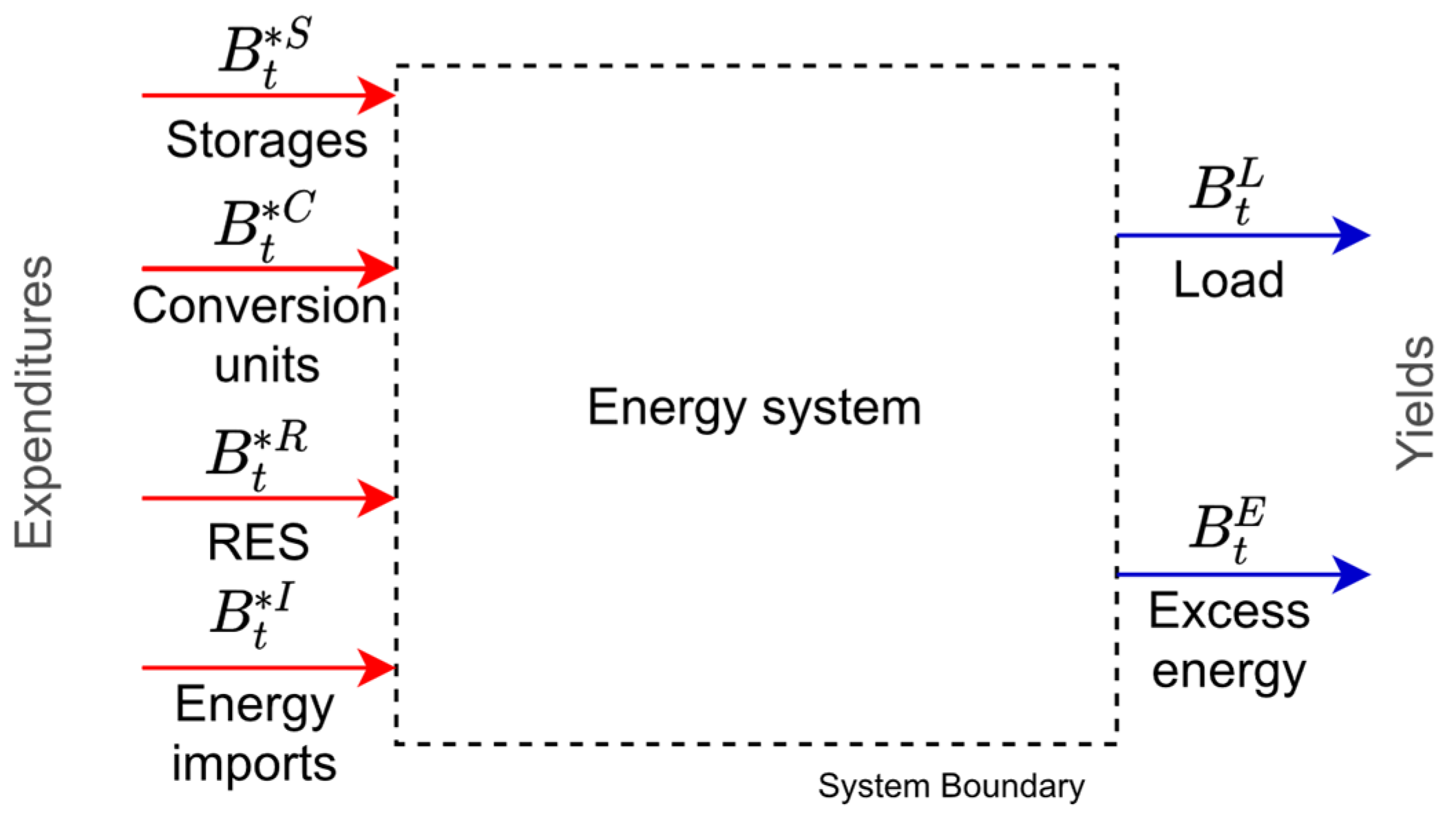
3.3.1. Energy Imports, Loads and Excess Energy

Imports, loads and excess energy are flows of energy carriers over the system boundary, for example electricity or gas exchange with their respective slacks (Figure 2). To model those, the oemof components source and sink are used. Imports are flows of pre-processed energy carriers such as electricity, natural gas, biomass or industrial waste heat into the energy system. They have a maximum power $P_{i,max}^I$ constraint (Equation (10)) and the CExC $B_i^{*I}$ is added to the objective function (Equation (11)). No investment expenditures are incurred, as they are already included in the CExC-factor $r_i^{*I}$.

$$P_i^I\left(t\right)-P_{i,max}^I\left(t\right)\le 0$$

(10)

$$B_i^{*I}=\sum _t{P}_i^I\left(t\right)·r_i^{*I}·\tau$$

(11)

Loads are flows of energy carriers to the consumers, for example electricity, process heat or domestic heat. The demand time-series are given, and therefore, the actual values $P_{l,actv}^L$ of any load is prescribed (Equation (12)). The yield $B_l^L$ is the exergy delivered to the consumer (Equation (13)):

$$P_l^L\left(t\right)-P_{l,actv}^L\left(t\right)=0$$

(12)

$$B_l^L=\sum _t{P}_l^L\left(t\right)·r·\tau$$

(13)

Excess energy $P_e^E$ are energy carriers that are neither consumed nor stored locally and are returned to the grid. In our case this only applies to electricity. Excess energy has a maximum power $P_{e,max}^E$ constraint (Equation (14)). The yield is the exergy $B_e^E$ stored in the energy carrier (Equation (15)).

$$P_e^E\left(t\right)-P_{e,max}^E\left(t\right)\le 0$$

(14)

$$B_e^E=\sum _t{P}_e^E\left(t\right)·r_e^E·\tau$$

(15)

3.3.2. RES

RES includes electricity produced by wind and PV. Their time-series are given, and therefore, an actual value $P_{r,actv}^R$ is prescribed (Equation (16)). Since RES potentials are usually limited, a maximum capacity $P_{r,inst, max}^R$ constraint is added (Equation (17)). RES CExC $B_r^{*R}$ comprise both investment and operating expenditures (Equation (18)). In the case of RES, the CExC-factor is equal to the exergy-factor $r_r^R$ [53].

$$P_r^R\left(t\right)-P_{r,actv}^R\left(t\right)=0$$

(16)

$$P_{r,inst}^R-P_{r,inst, max}^R \le 0$$

(17)

$$B_r^{*R}=P_{r,inst}^R·r_r^{*p,R}+\sum _t{P}_r^R\left(t\right)·r_r^R·\tau$$

(18)

3.3.3. Conversion Units

Conversion units such as boilers, CHPs or heat pumps can have single or multiple inputs $P_{c,in}$ and outputs $P_{c,out}$. For a set of different energy carriers α, β, … ∈ Γ = {electricity, natural gas, heat, hydrogen, biomass, …}, energy conversion is modelled using a conversion matrix $C_c$, which consists of the conversion efficiencies ${\eta }_c$ [33]. Therefore, the following constraints are added:

$$\underset{P_{c,out}}{\underbrace{\left(\begin{array}{c}{P}_{c,out}^{\alpha }\left(t\right)\\ P_{c,out}^{\beta }\left(t\right)\\ ⋮\\ P_{c,out}^{\omega }\left(t\right)\end{array}\right)}}=\underset{C_c}{\underbrace{\left(\begin{array}{cccc}{\eta }_c^{\alpha ,\alpha }& {\eta }_c^{\beta ,\alpha }& \cdots & {\eta }_c^{\omega ,\alpha }\\ {\eta }_c^{\alpha ,\beta }& {\eta }_c^{\beta ,\beta }& \cdots & {\eta }_c^{\omega ,\beta }\\ ⋮& ⋮& \ddots & ⋮\\ {\eta }_c^{\alpha ,\omega }& {\eta }_c^{\beta ,\omega }& \cdots & {\eta }_c^{\omega ,\omega }\end{array}\right)}}*\underset{P_{c,in}}{\underbrace{\left(\begin{array}{c}{P}_{c,in}^{\alpha }\left(t\right)\\ P_{c,in}^{\beta }\left(t\right)\\ ⋮\\ P_{c,in}^{\omega }\left(t\right)\end{array}\right)}}$$

(19)

As there are several interdependent inputs and outputs, one of them must be defined as a reference $P_{c,ref}^C$. The installed capacity $P_{c,inst}^C$ and the equivalent periodic CExC-factor $r_c^{*p,C}$ refer to this reference. The reference input or output must be always less than or equal to the installed capacity (Equation (20)). The expenditures are the CExC B^*C necessary to install a conversion unit (Equation (21)):

$$P_{c,ref}^C\left(t\right)-P_{c,inst}^C\le 0$$

(20)

$$B_c^{*C}=P_{c,inst}^C·r_c^{*p,C}$$

(21)

3.3.4. Storages

A differential energy balance between two consecutive timesteps is used to model energy storage. The change in state of energy $SO{E}_s$ describes the currently stored energy, where ${\eta }_{s,in}$ and ${\eta }_{s,out}$ are the input and output efficiencies and ${\eta }_{s,loss}$ are the standby losses:

$$∆SO{E}_s\left(t\right)=\left[{\eta }_{s,in}·P_{s,in}\left(t\right)-{\eta }_{s,out}·P_{s,out}\left(t\right)\right]·\tau -{\eta }_{s,loss}·SO{E}_s\left(t-1\right)$$

(22)

The current $SO{E}_s$ of energy must always be less than or equal to the installed capacity $C_{s,inst}^S$ (Equation (23)). The expenditures are the CExC $B_s^{*S}$ necessary to install a conversion unit (Equation (24)):

$$SO{E}_s\left(t\right)-C_{s,inst}^S\le 0$$

(23)

$$B_s^{*S}=C_{s, inst}^S·r_s^{*p,S}$$

(24)

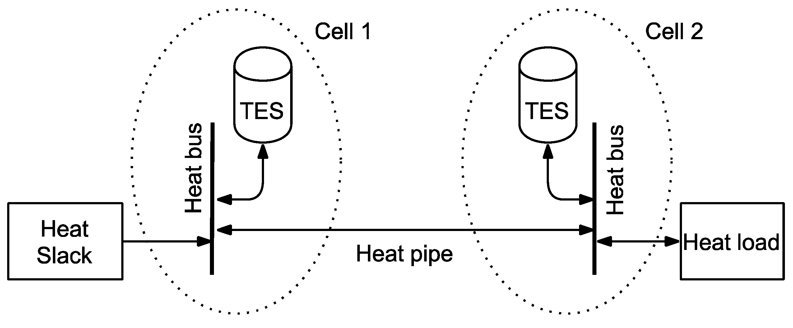
3.3.5. Energy Transmission

For energy transmission, two different models are compared. Basic and simplified network flow models are compared with higher detail power flow models. The network flow models only consider energy losses and are equivalent for all energy carriers. The power flow models also consider the driving potential such as voltage or pressure in electricity, heat and natural gas grids, respectively.

Network flow models only use two constraints. One describes the transmission losses using the transmission efficiency ${\eta }_t^T$ (Equation (25)). The other one limits the maximum capacity $P_{t,max}^T$ (Equation (26)):

$$P_{t,in}^T\left(t\right)·{\eta }_t^T-P_{t,out}^T\left(t\right)=0$$

(25)

$$P_{t,in}^T\left(t\right)-P_{t,max}^T\le 0$$

(26)

The power flow models require additional constraints representing the physical power flow relations. For the electricity flows we assume that the ohmic resistance $R$ is negligibly small compared to the reactance $X_t^T$. In such a case, we can use a DC-approximated power flow model [11], where the transmitted power $P_t^{T,el}$ is only dependent on the voltage angles ${\mathsf{\Theta }}_{t,in}^{T,el}$ and ${\mathsf{\Theta }}_{t,out}^{T,el}$, and the reactance $X_t^{T,el}$:

$$P_t^{T,el}\left(t\right)=\frac{{\mathsf{\Theta }}_{t,in}^{T,el}-{\mathsf{\Theta }}_{t,out}^{T,el}}{X_t^{T,el}}$$

(27)

For heat and natural gas flows the non-linear relationship between power $P_t^{T,g,h}$ and pressure drop ($p_{t,in}^{T,g,h}$, $p_{t,out}^{T,g,h}$) is represented by piecewise linearised functions. The resistance $R_t^{T,g,h}$ depends on the properties of the pipe ${\mathsf{\Phi }}_{\mathrm{t}}^P$ (diameter, length, roughness, etc.) and the fluid ${\mathsf{\Phi }}_{\mathrm{t}}^F$ (pressure, temperature, composition). A detailed derivation is shown in the Appendix A.

$$P_t^{T,g,h}\left(t\right)=\frac{\sqrt{p_{t,in}^{T,g,h}-p_{t,out}^{T,g,h}}}{R_t^{T,g,h}\left({\mathsf{\Phi }}_{\mathrm{t}}^P,{\mathsf{\Phi }}_{\mathrm{t}}^F\right)}$$

(28)

3.3.6. Busses

All components such as conversion units, storages or transmission lines are connected via busses in which all power flows ($P_{b,in}^B$, $P_{b,out}^B$) are balanced. Therefore, we add the following constraint for any bus:

$$\sum _{in}{P}_{b,in}^B\left(t\right)-\sum _{out}{P}_{b,out}^B\left(t\right)=0$$

(29)

For the power flow models, additional constraints are necessary. They balance and limit voltage angles and pressure levels. At any electrical bus just one voltage angle ${\mathsf{\Theta }}_{\mathrm{b}}^{B,el}$ is allowed, which is equal to the voltage angles of all inflows ${\mathsf{\Theta }}_{b,in}^{B,el}$ and outflows ${\mathsf{\Theta }}_{b,out}^{B,el}$ (Equation (30)). The voltage angles must stay within their bounds of ${\mathsf{\Theta }}_{b,min}^{B.el}$ and ${\mathsf{\Theta }}_{b,max}^{B,el}$ (Equation (31)):

$${\mathsf{\Theta }}_{\mathrm{b}}^{B,el}\left(t\right)={\mathsf{\Theta }}_{b,in}^{B,el}\left(t\right)={\mathsf{\Theta }}_{b,out}^{B,el}\left(t\right)$$

(30)

$${\mathsf{\Theta }}_{b,min}^{B.el}\le {\mathsf{\Theta }}_{\mathrm{b}}^{B,el}\left(t\right)\le {\mathsf{\Theta }}_{b,max}^{B,el}$$

(31)

For heat and natural gas networks the same rules apply for the pressure level $p_b^{B,g,h}$ in the busses:

$$p_b^{B,g,h}\left(t\right)=p_{b,in}^{B,g,h}\left(t\right)=p_{b,out}^{B,g,h}\left(t\right)$$

(32)

$$p_{b,min}^{B,g,h}\le p_b^{B,g,h}\left(t\right)\le p_{b,max}^{B,g,h}$$

(33)

4. Case Study

We have designed a case study that aims to answer our research questions. It combines CExC-minimisation, a multi-cell energy system and network and power flow representations. For a given demand, grid capacities and renewable potentials, the optimal operation and installed capacities of energy conversion units and storage facilities shall be determined. The different results of the network flow(NF) model and the power flow (PF) model will be discussed.

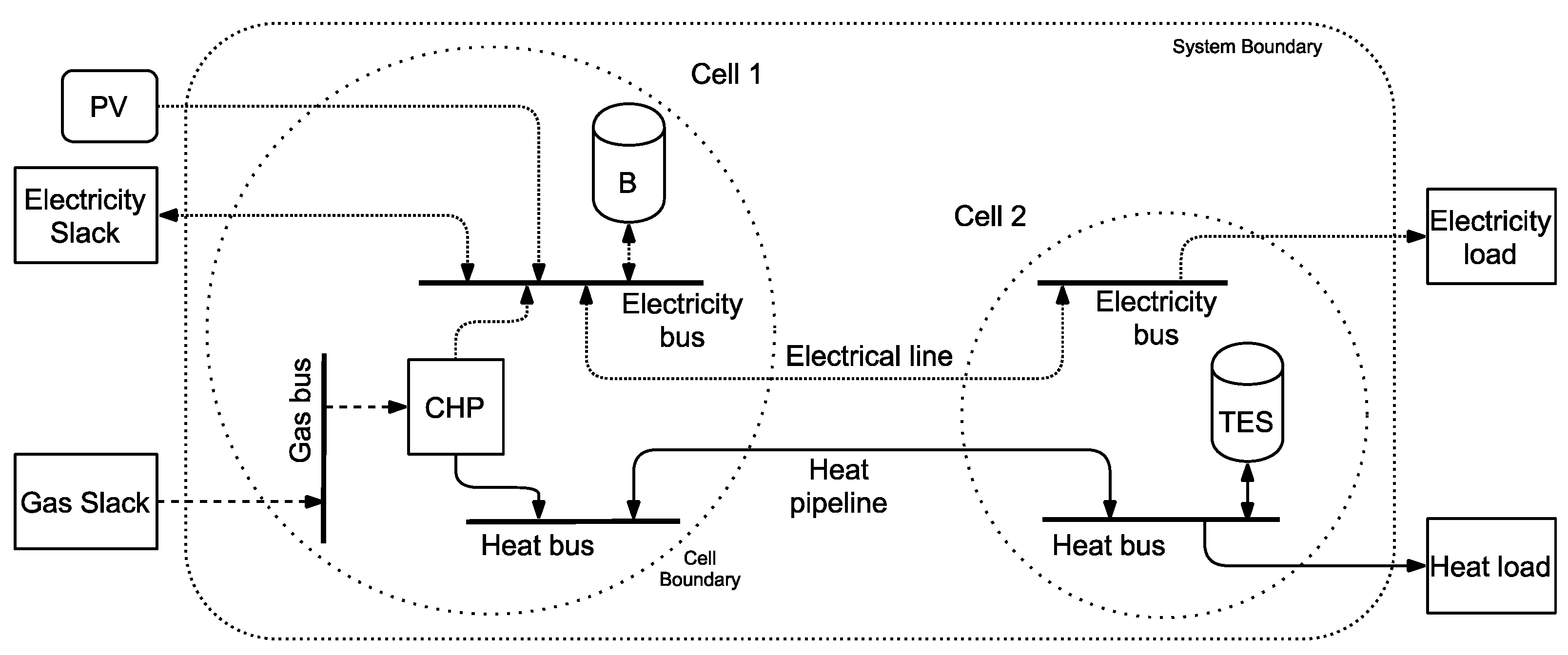
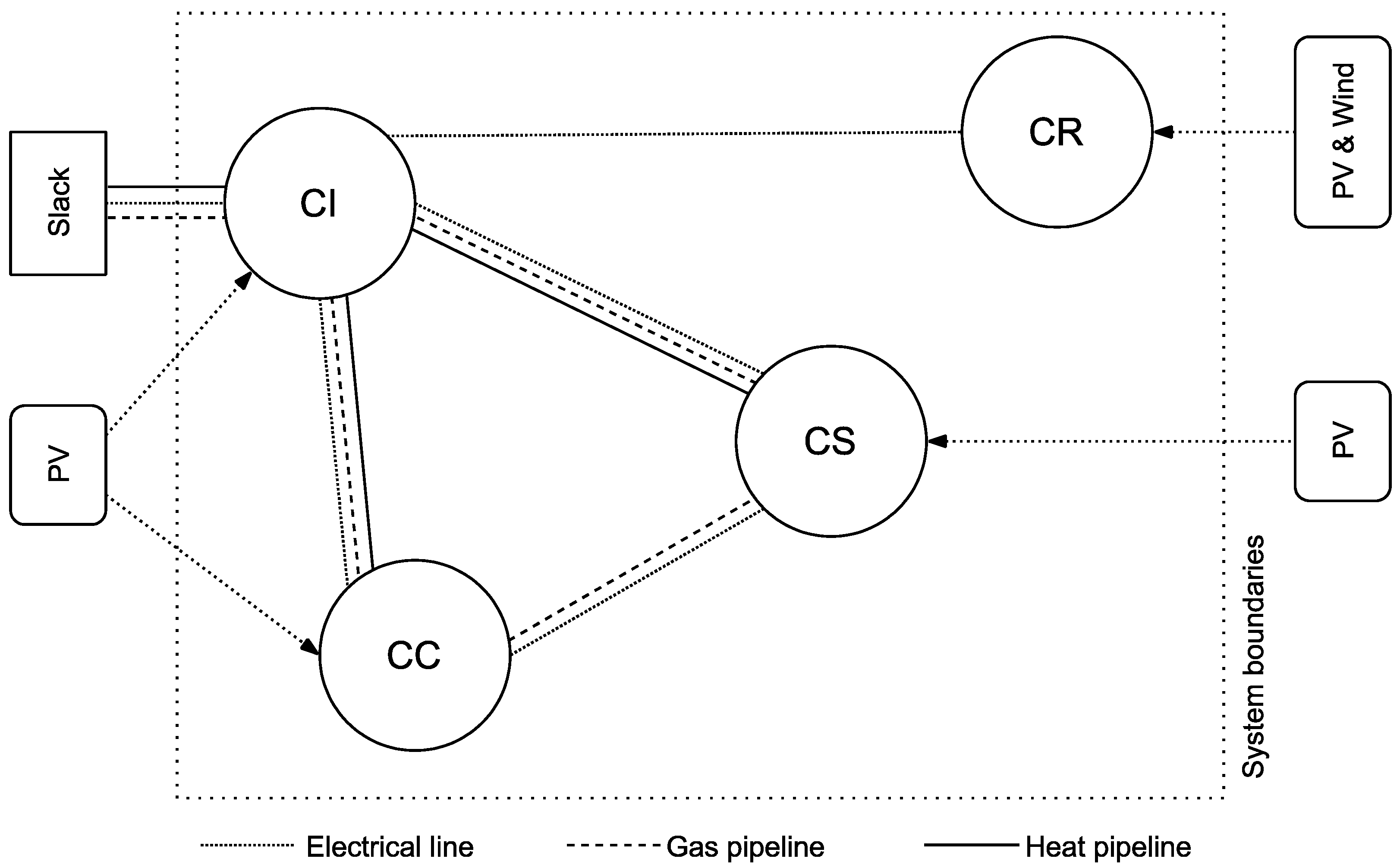
4.1. System Description

We use a simplified model city, which is divided into four cells. Simplification is carried out according to the cellular approach [29]. The cells represent the areas typical for a city: city centre (CC), suburbs (CS), industrial areas (CI) and rural areas (CR) (Figure 3). In any cell, a range of conversion technology, storages and RES for possible installation is provided. We use the same components as used in [27]: battery, thermal energy storage (TES), H₂-Storage, PV, wind, biomass boiler, gas boiler, heat pump, PEM electrolyser, PEM fuel cell, resistance heater, biomass CHP, gas CHP. All relevant data such as efficiencies and equivalent periodic CExC factors are overtaken from there. Tables presenting this data are provided in the Appendix B.

Each imported energy carrier (electricity and natural gas from the transmission grids, waste heat from an industrial plant, biomass from the rural areas) needs to be assessed by its CExC-factor (

Table 1. CExC-factors for the different imported energy carriers [27].

	Electricity	Natural Gas	Waste Heat	Biomass
CExC-factor $r_i^I$ in $\frac{MWh}{MWh}$	2.0	1.21	0.21	1.1

). Again, we apply the values of [27], which correspond to the current CExC-factors. An exception is made for electricity. The current CExC-factor is 2.96, but we use a lower value of 2 because this already corresponds to a future energy system with a higher share of renewable energy sources.

The connection to the slack nodes for energy import is in CI. While the connection for electricity is bidirectional, gas and waste heat can only be obtained from the source. The cells are connected by electricity, natural gas and heat grids. While all cells are covered by the electricity grid, only the denser populated cells are connected to the natural gas and heat grids. Maximum transmission capacities and efficiencies can be found in

Table 2. Installed slack node capacities and installed grid capacities and efficiencies.

		Electricity	Natural Gas	Heat
CI-Slack	Max. cap. $P_{CI-S,max}^I$	600 MW	1000 MW	20 MW
CI-CC	Max. cap. $P_{CI-CC,max}^T$	36 MW	163 MW	30 MW
	Efficiency ${\eta }_{CI-CC}^T$	99.9%	99.9%	85%
CI-CS	Max. cap. $P_{CI-CS,max}^T$	36 MW	141 MW	30 MW
	Efficiency ${\eta }_{CI-CS}^T$	99.9%	99.9%	85%
CC-CS	Max. cap. $P_{CC-CS,max}^T$	36 MW	100 MW
	Efficiency ${\eta }_{CC-CS}^T$	99.9%	99.9%
CI-CR	Max. cap. $P_{CI-CR,max}^T$	36 MW
	Efficiency ${\eta }_{CI-CR}^T$	99.9%

.

While maximum capacities and transmission capacities are sufficient for the network flow, we also need the line and pipeline lengths, reactances $X_t^{T,el}$ and the pressure drops at maximum heat and gas load ($\Delta p_{t, max}^{T,g}$, $\Delta p_{t, max}^{T,h}$) for the power flow calculations (

Table 3. Lengths, reactances and pressure drops for the power flow calculations.

	$\mathbf{Length}{\mathit{l}}_{\mathit{t}}^{\mathit{T}}$	$\mathbf{Reactance}{\mathit{X}}_{\mathit{t}}^{\mathit{T},\mathit{e}\mathit{l}}$	$\mathbf{Pressure}\mathbf{Drop}\mathbf{Gas}\mathsf{\Delta }{\mathit{p}}_{\mathit{t}, \mathit{m}\mathit{a}\mathit{x}}^{\mathit{T},\mathit{g}}$	$\mathbf{Pressure}\mathbf{Drop}\mathbf{Heat} \mathsf{\Delta }{\mathit{p}}_{\mathit{t}, \mathit{m}\mathit{a}\mathit{x}}^{\mathit{T},\mathit{h}}$
	$\mathit{k}\mathit{m}$	$\mathit{W}/\mathit{k}\mathit{m}$	$\mathit{m}\mathit{b}\mathit{a}\mathit{r}$	$\mathit{m}\mathit{b}\mathit{a}\mathit{r}$
CI-CC	2.5	0.0729	40.5	119.1
CI-CS	5.0	0.0729	40.5	119.1
CC-CS	7.5	0.0729	40.5
CI-CR	10.0	0.0729

). The normalised power–pressure drop relation (

Table A1. Pipe properties.

	Heat Pipe	Gas Pipe
Diameter	350 mm	300 mm
Length	1000 m	1000 m
Temperature difference Supply/return	50 °C
Gross calorific value		11 kWh/Nm3
Pipe roughness	1 mm	0.3 mm
Max. power	50 MW	163 MW

) is denormalised using the maximum capacities (Table 2) and the corresponding maximum pressure drops (Table 3).

For any cell electricity and domestic or process heat, time series are created based on the annual demand $E_l^L$ (

Table 4. Annual demand, annual RES potentials and the corresponding maximum power per cell.

Cell			Electricity	Domestic Heat	Process Heat	PV	Wind
CC	Ann. Demand $E_{CC}^L$	GWh	137.5	405.0		31.8
	Max. Power $P_{CC,max}^L$	MW	26.1	162.2		62.5
CS	Ann. Demand $E_{CS}^L$	GWh	110.0	315.0		65.5
	Max. Power $P_{CS,max}^L$	MW	20.9	140.4		50
CI	Ann. Demand $E_{CI}^L$	GWh	220.0		72.0	130.9
	Max. Power $P_{CI,max}^L$	MW	52.8		22.1	100
CR	Ann. Demand $E_{CR}^L$	GWh	82.5	180.0		49.1	697.1
	Max. Power $P_{CR,max}^L$	MW	17.6	92.5		37.5	330

). In total, 80% of the process heat is considered to be waste heat and can be further utilised for domestic heating. To create time series with a resolution of 15 min, the load profile generator oemof.demandlib [54] was used. For any cell, a maximum potential for PV and wind RES was assumed. Time series were obtained using renewables.ninja (location: latitude: 47.84, longitude: 16.54; year 2014) [55,56].

4.2. Results

The results show two basic, but different findings. The total CExC-expenditures and total installed capacities show only minor differences for both cases. Nevertheless, the capacities of the installed components in the individual cells differ significantly from the NF to PF case.

The largest deviations occur in the capacities of heat pumps, CHP, TES and batteries in the well meshed CC and CS cells. Nevertheless, summed up over all cells, the installed conversion unit capacities differ only marginally (see gap in

Table 5. Installed conversion unit capacities $P_{c,inst}^C$ and RES capacities $P_{r,inst}^R$.

		CI	CC	CS	CR	Total	Gap
		MW	MW	MW	MW	MW	MW
Gas boiler PH	NF	22.1				22.1	0.0
	PF	22.1				22.1
Resistance heater PH	NF	20.8				20.8	0.0
	PF	20.8				20.8
Heat pump	NF		163.0	145.4	240.2	548.6	+1.8
	PF		138.8	171.6	240.0	550.4
Biomass CHP	NF		7.1			7.1	+3.9
	PF		11.0			11.0
Fuel Cell	NF				20.0	20.0	0.0
	PF				20.0	20.0
Electrolyser	NF				66.3	66.3	−0.2
	PF				66.1	66.1
Wind	NF				214.9	214.9	+0.1
	PF				215.0	215.0
PV	NF	100	62.5	50		212.5	0.0
	PF	100	62.5	50		212.5

). The biggest difference in total installed capacity is for the CHP plant in CC. In most cases lower installed capacities are obtained with the NF model than with the PF case. The same applies to the installed storage capacities (

Table 6. Installed storage capacities $P_{s,inst}^S$.

		CI	CC	CS	CR	Total	Gap
		MWh	MWh	MWh	MWh	MWh	MWh
Battery	NF	22.0	96.3	73.1	443.3	634.7	+1.5
	PF	22.0	162.5	6.9	444.8	636.2
TES	NF		1340.0	1625.2	8614.2	11579.4	−15.8
	PF		1728.8	1219.7	8614.2	11,563.6
H2 storage	NF				13,474.0	13,474.0	−12.8
	PF				13,461.2	13,461.2

). Here, the power flow model provides the lower installed capacities, except for the battery.

In the poorly interconnected cells such as CR or the process heat production the installed capacities hardly differ, neither in the conversion units nor in the storages. Overall, apart from process heat production where gas boilers and resistance heaters are used, only exergy-efficient technology such as CHP and heat pumps are used for domestic heat production.

For operational analysis and comparison, we apply statistical methods on the time series of the installed components. The parameters calculated for conversion units, powerlines, and pipes include the mean power $P_{x,m}^X$, the minimum power $P_{x,min}^X$, the maximum power $P_{x,max}^X$ and the median power $P_{x,md}^X$. Additionally, we calculated the capacity factor $c_{x,F}^X$. For the storages we carried out the same calculations using the state of energies ($SOE$). Instead of the capacity factor, we calculated the number of annual storage cycles $c_{x,SC}^X$. The results are presented in

Table 7. Statistical analysis of the conversion unit and RES timeseries.

			${\mathit{c}}_{\mathit{c},\mathit{F}}^{\mathit{C}}$	${\mathit{P}}_{\mathit{c},\mathit{m}}^{\mathit{C}}$	${\mathit{P}}_{\mathit{c},\mathit{m}\mathit{i}\mathit{n}}^{\mathit{C}}$	${\mathit{P}}_{\mathit{c},\mathit{m}\mathit{a}\mathit{x}}^{\mathit{C}}$	${\mathit{P}}_{\mathit{c},\mathit{m}\mathit{d}}^{\mathit{C}}$
			-	$\mathit{M}\mathit{W}$	$\mathit{M}\mathit{W}$	$\mathit{M}\mathit{W}$	$\mathit{M}\mathit{W}$
CI	Gas boiler PH	NF	0.39	8.6	0.0	22.1	8.4
		PF	0.39	8.6	0.0	22.1	8.4
	Resistance heater PH	NF	0.08	1.7	0.0	20.8	0.0
		PF	0.08	1.7	0.0	20.8	0.0
	PV	NF	0.15	14.9	0.0	85.0	0.5
		PF	0.15	14.9	0.0	85.0	0.5
CC	Heat Pump	NF	0.21	34.2	0.0	163.0	0.3
		PF	0.23	31.9	0.0	138.8	3.7
	Biomass CHP	NF	0.05	0.4	0.0	7.1	0.0
		PF	0.10	1.1	0.0	11.0	0.0
	PV	NF	0.15	9.3	0.0	53.1	0.3
		PF	0.15	9.3	0.0	53.1	0.3
CS	Heat Pump	NF	0.20	29.4	0.0	145.4	0.0
		PF	0.18	30.7	0.0	171.6	0.0
	PV	NF	0.15	7.5	0.0	42.5	0.3
		PF	0.15	7.5	0.0	42.5	0.3
CR	Heat Pump	NF	0.09	21.8	0.0	240.2	0.0
		PF	0.09	21.8	0.0	240.0	0.0
	Fuel Cell	NF	0.26	6.9	0.0	26.7	0.0
		PF	0.26	6.9	0.0	26.7	0.0
	Electrolyser	NF	0.11	5.1	0.0	20.0	0.0
		PF	0.11	5.1	0.0	20.0	0.0
	Wind	NF	0.24	51.8	0.1	212.9	39.6
		PF	0.24	51.8	0.1	212.9	39.6

,

Table 8. Statistical analysis of the storages’ SOE time series.

			${\mathit{c}}_{\mathit{s},\mathit{S}\mathit{C}}^{\mathit{S}}$	$\mathit{S}\mathit{O}{\mathit{E}}_{\mathit{s},\mathit{m}}^{\mathit{S}}$	$\mathit{S}\mathit{O}{\mathit{E}}_{\mathit{s},\mathit{m}\mathit{i}\mathit{n}}^{\mathit{S}}$	$\mathit{S}\mathit{O}{\mathit{E}}_{\mathit{s},\mathit{m}\mathit{a}\mathit{x}}^{\mathit{S}}$	$\mathit{S}\mathit{O}{\mathit{E}}_{\mathit{s},\mathit{m}\mathit{d}}^{\mathit{S}}$
			-	$\mathit{M}\mathit{W}\mathit{h}$	$\mathit{M}\mathit{W}\mathit{h}$	$\mathit{M}\mathit{W}\mathit{h}$	$\mathit{M}\mathit{W}\mathit{h}$
CI	Battery	NF	108.1	3.9	0	22.0	0.0
		PF	135.4	4.7	0	22.0	0.0
CC	Battery	NF	131.8	50.6	0	96.3	51.7
		PF	129.2	82.5	0	162.5	79.1
	TES	NF	55.6	285.5	0	1339.8	138.7
		PF	50.9	327.8	0	1728.8	153.8
CS	Battery	NF	137.1	38.8	0	73.1	39.4
		PF	128.7	3.4	0	6.9	2.9
	TES	NF	40.0	297.3	0	1625.2	125.1
		PF	38.9	204.3	0	1219.7	32.3
CR	Battery	NF	72.4	221.9	0	443.3	212.2
		PF	72.8	277.9	0	444.8	303.0
	TES	NF	13.2	1583.5	0	8614.2	692.7
		PF	13.2	1577.5	0	8614.2	684.7
	H2-storage	NF	4.5	8738.7	0	13,474.0	9881.4
		PF	4.5	8698.5	0	13,461.2	9823.1

and

Table 9. Statistical analysis of the powerline and heat pipeline time series.

		${\mathit{P}}_{\mathit{t},\mathit{m}}^{\mathit{T}}$	${\mathit{P}}_{\mathit{t},\mathit{m}\mathit{i}\mathit{n}}^{\mathit{T}}$	${\mathit{P}}_{\mathit{t},\mathit{m}\mathit{a}\mathit{x}}^{\mathit{T}}$	${\mathit{P}}_{\mathit{t},\mathit{m}\mathit{d}}^{\mathit{T}}$
		$\mathit{M}\mathit{W}$	$\mathit{M}\mathit{W}$	$\mathit{M}\mathit{W}$	$\mathit{M}\mathit{W}$
CI-CC Heat	NF	11.8	0.0	20.8	13.4
	PF	13.1	0.0	20.8	10.7
CI-CS Heat	NF	6.8	0.0	20.5	6.8
	PF	5.4	0.0	20.8	6.4
CC-CS Electricity	NF	−0.1	−5.9	0.0	0.0
	PF	2.3	−16.6	18.4	1.7
CI-CC Electricity	NF	17.8	−27.2	36.0	14.7
	PF	19.1	−31.7	36.0	18.9
CI-CR Electricity	NF	−29.6	−36.0	36.0	−36.0
	PF	−29.6	−36.0	36.0	−36.0
CI-CS Electricity	NF	15.4	−21.1	36.0	11.2
	PF	13.0	−20.2	36.0	10.7

.

The data shows comparable capacity factors for the NF and PF case. Capacity factors for most conversion units and RES range from 0.05 to 0.26. Exceptional is only the gas burner with 0.39 and the gap for the biomass CHP between the NF and PF case. For all conversion units except for the process heat gas boiler and the heat pump in CC, median values are zero. This means that they are switched off for at least half of the time.

Storage cycles differ for all storages between NF and PF, with the exception of TES and H2-storage in CR. In the well meshed cells CI, CC and CS batteries and TES show higher storage cycles compared to CR. The mean TES’ SOE ranges from 17% to 21% of its maximum SOE. For batteries, this value ranges from 49% to 62% in CC, CS and CR, and 18% to 21% in CI. The battery in CI is also the only storage that is empty for more than 50% of the time (median is zero).

The normalised load duration curves and boxplots in Figure 4 show changes between the NF and PF model in all load flows except for the electrical stub line CI-CR. The occurring maximum values in both directions stay the same for all load flows, apart from CC-CS. The electrical line CC-CS is barely used in the NF case. The direct electricity flows from CI to CS in the NF case are partially rerouted in the PF case. This leads to higher flows through CI-CC and CC-CS and reduced flows through CI-CS. This can be seen from the shifted boxes in the box plot (Figure 4) and the changed mean values (Table 9). Those changed electricity flows also cause a better utilisation of the CI-CC heat pipeline at the expense of the CI-CS pipeline (Table 9).

The overall results show a total CExC-expenditures increase by 0.1% in the PF case compared to the NF case (

Table 10. CExC expenditures and yields.

	Expenditures in GWh				Yields in GWh
	RES	Import	Infrastructure	Total	Load	Excess	Total
NW	732.1	454.8	133.3	1320.2	766.0	19.9	785.9
PF	732.2	455.7	133.6	1321.5	766.0	19.9	785.9

). These are due to increased energy imports and higher infrastructure expenditures (+0.2% each). Electricity imports decrease (−5.8% compared to NF), while the biomass increases by 1.9 times (

Table 11. CExC for the imported energy carriers.

	Electricity	Gas	Heat	Biomass
	GWh	GWh	GWh	GWh
NF	312.6	95.9	36.4	9.9
PF	294.5	95.9	36.4	28.9

). The yields do not differ for both cases.

5. Discussion and Conclusions

First, we will discuss the results and analyse the reasons for the differences between the results of the NF and PF models. Then we will close this section with a conclusion and an outlook.

5.1. Model Discussion and Comparison

The difference of only 0.1% shows that the two different load flow models only have a minor impact on the overall results. The same conversion and storage technology systems are selected for the NF and PF models, but there are differences in the installed capacities and the operating behaviour. In cells at the end of stub lines, such as CR or the process heat demand in CI, the installed capacities and the operational statistical parameters hardly change at all. The main differences occur in the well meshed cells CC and CS (compare Table 5, Table 6, Table 7, Table 8 and Table 9).

In NF models, the flows from one to another cell are independent from any other flow and are only restricted by the maximum capacity. In PF models all flows are linked by the power flow equations leading to specific voltage angles and pressure levels in the respective busses. Compared to the NF calculations, this leads to changes in load flows and the installed capacities of heat pumps and storages in the CC and CS cells. To fulfil the load flow equations in the PF case, the direct electricity flows from CI to CS are reduced, but they are rerouted via CI-CC and CC-CS. The CC-CS line is hardly used in the NF case (Figure 4). In the PF case, this rerouting causes an increased heat pump capacity and decreased battery and TES capacities in CS. For CC it is vice-versa.

The component with the most significant differences between NF and PF is the CHP in CC. The total installed capacity and operational statistical parameters differ between the NF and PF case like for no other component. Its capacity increases by 55% and its capacity factor doubles compared to the NF case. In the PF case the CHP is needed in times of high heat and power demand in CS and CC. Then the powerlines from CI to CC and CS are fully loaded. To satisfy the load flow equations, a flow from CC to CS must also be established, which is provided by the CHP. The load duration curve shows this state in Figure 4 with a small horizontal section at 79.4% of the maximum transmission capacity.

In the well meshed inner parts of the city (CI, CS, CC) the capacity factors of heat pumps (01.18–0.23 to 0.09) and the annual storage cycles for batteries (108.1–137.1 to 72.4–72.8) and TES (38.9–55.6 to 13.2) are higher than in cell CR for the NF and PF case (Table 7 and Table 8). This is caused by the lower demand to RES potential ratio in the inner cells compared to the rural cell CR and the limited network connection of CR. Due to excess energy, this leads to lower operational expenditures for energy production and therefore allows higher infrastructure expenditures. This is analogous to results for a nodal pricing scheme in the electricity market [57].

Data in Table 10 shows that the use of the NF or PF model does not lead to significant differences in expenditures and yields. Additionally, operating and investment expenditures remain in the same order of magnitude. Even though the total expenditures for energy import only change by $0.9 GWh$ (this is equivalent to 0.2%), in the PF case there is a shift from electricity imports to biomass imports. This is caused by the biomass CHP, which must be installed in CC due to the load flow equations in the PF case.

In the real world, the high and medium voltage levels of electricity grids can be regarded as heavily meshed. Low-voltage networks are also built as meshed networks but are operated as radial networks for reasons of easier fault clearance. Large scale district heating networks are usually meshed, smaller ones are implemented as radial networks [58]. High pressure transmission gas networks are operated as radial networks, but the low pressure distribution grids are meshed [59]. Based on the results of the case studies, general recommendations for the modelling of different network levels and types can be derived (

Table 12. Proposed use of NF and PF for different energy carriers and types of networks.

		NF	PF
Electricity grids	High voltage/transmission		X
	Medium voltage/distribution		X
	Low voltage/distribution	X
District heating networks	Large scale		X
	Small scale	X
Gas networks	High pressure/transmission	X
	Low pressure/distribution		X

): PF models best reflect meshed networks, NF models offer insight to radial networks and stub lines.

5.2. Conclusion and Outlook

This work compares NF and PF formulations for the optimum installed conversion unit and storage capacities in a multi-cell municipal energy system model. The results show that the total CExC-expenditures for both approaches are in the same order of magnitude. However, on a cellular level there occur differences in installed storage and conversion unit capacities, especially in well-meshed cells. More detail in the model delivers more accurate results, but also requires more input parameters (which are not always available) and is computationally more expensive. For our models, computation times were in the range of one to several hours for the NF model and in the range of one to several days for the PF model (used system configuration: 32-core AMD Ryzen Threadripper 2990WX with 128GB RAM). Parametrisation of components in a multi-cell model has major impacts on computation times and result quality. Further details are provided in Appendix C.

In general, NF-like models are often used for large scale energy system models, for example in a scenario analysis for the future configuration of Great Britain’s power system [60]. In the context of optimal system design, PF models are employed for electricity grid specific applications, like the long term capacity planning in Switzerland [61]. Which energy transmission representation to select for a certain model depends on the objective and purpose of the task, the available input data and the energy grid design. In radial networks, differences between an NF and PF approach will be smaller than in meshed networks.

The basic concept of CExC-minimisation was presented in [27]. In the current work we added the spatial dimension by investigating two different grid representations. Future research fields may concern the methodology and input data as well as the application of the methodology on different sectors. Improvements to the methodology include the implementation of further RES, conversion and storage technology. There is also the possibility that DSM can reduce the necessary storage capacity. Through stochastic modelling, variable RES can be modelled more realistically.

For the input data, the quality of the CExC-factors is crucial. This applies to the parameters themselves, as well as to the accuracy of the modelling. At the moment we mainly use data from the life cycle assessment database ProBas [62], a comparison to the data from other databases such as ecoinvent [63] can be beneficial. At the time of writing, all CExC-factors are constant. However, for electricity it will vary over the day and the year depending on the supply of RES. The same applies for the demand, which is currently also modelled-fixed.

The methodology is so general that future applications will cover a wide field. This ranges from small energy systems such as houses to larger energy systems such as entire countries. In our case study, we only modelled the domestic sector, which includes households, small businesses and governmental organisations. In particular, the inclusion of the transport sector (electromobility) and the industrial sector can reveal additional synergies.

References

1. European Commission. Energy Roadmap 2050. Communication from the Commission to the European Parliament, the Council, the European Economic and Social Committee and the Committee of the Regions; 885 Brussels, Belgium, 2011; European Commission: Brussels, Belgium, 2011. [Google Scholar]
2. Eurostat. Energy Balances. Available online: https://ec.europa.eu/eurostat/web/energy/data/energy-balances (accessed on 6 November 2019).
3. Sejkora, C.; Kienberger, T. Dekarbonisierung der Industrie mithilfe elektrischer Energie? In 15. Symposium Energieinnovation; Technische Universität Graz: Graz, Austria, 2018. [Google Scholar]
4. Geyer, R.; Knöttner, S.; Diendorfer, C.; Drexler-Schmid, G. IndustRiES. Energieinfrastruktur Für 100% Erneuerbare Energie in der Industrie; Klima-und Energiefonds der österreichischen Bundesregierung: Wien, Austria, 2019. [Google Scholar]
5. Wall, G. Exergy. A Useful Concept; TH: Göteborg, Sweden, 1986; ISBN 9170322694. [Google Scholar]
6. International Energy Agency. Key World Energy Statistics. Also Available on Smartphones and Tablets; International Energy Agency: Paris, France, 2017. [Google Scholar]
7. Statistik Austria. Nutzenergieanalyse (NEA). 2017. Available online: http://www.statistik.at/web_de/statistiken/energie_umwelt_innovation_mobilitaet/energie_und_umwelt/energie/nutzenergieanalyse/index.html (accessed on 18 January 2018).
8. Haas, R.; Panzer, C.; Resch, G.; Ragwitz, M.; Reece, G.; Held, A. A historical review of promotion strategies for electricity from renewable energy sources in EU countries. Renew. Sustain. Energy Rev. 2011, 15, 1003–1034. [Google Scholar] [CrossRef]
9. Kriechbaum, L.; Scheiber, G.; Kienberger, T. Grid-based multi-energy systems—modelling, assessment, open source modelling frameworks and challenges. Energ. Sustain. Soc. 2018, 8, 244. [Google Scholar] [CrossRef] [Green Version]
10. Sejkora, C.; Kühberger, L.; Radner, F.; Trattner, A.; Kienberger, T. Exergy as Criteria for Efficient Energy Systems—A Spatially Resolved Comparison of the Current Exergy Consumption, the Current Useful Exergy Demand and Renewable Exergy Potential. Energies 2020, 13, 843. [Google Scholar] [CrossRef] [Green Version]
11. Böckl, B.; Greiml, M.; Leitner, L.; Pichler, P.; Kriechbaum, L.; Kienberger, T. HyFlow—A Hybrid Load Flow-Modelling Framework to Evaluate the Effects of Energy Storage and Sector Coupling on the Electrical Load Flows. Energies 2019, 12, 956. [Google Scholar] [CrossRef] [Green Version]
12. Krause, T.; Kienzle, F.; Art, S.; Andersson, G. Maximizing exergy efficiency in multi-carrier energy systems. In Proceedings of the Energy Society General Meeting, Minneapolis, MN, USA, 25–29 July 2010; pp. 1–8. [Google Scholar]
13. Wall, G. Exergy tools. Proc. Inst. Mech. Eng. A J. Power Energy 2003, 217, 125–136. [Google Scholar] [CrossRef]
14. Dewulf, J.; van Langenhove, H.; Muys, B.; Bruers, S.; Bakshi, B.R.; Grubb, G.F.; Paulus, D.M.; Sciubba, E. Exergy: Its Potential and Limitations in Environmental Science and Technology. Environ. Sci. Technol. 2008, 42, 2221–2232. [Google Scholar] [CrossRef]
15. Tsatsaronis, G. Thermoeconomic analysis and optimization of energy systems. Prog. Energy Combust. Sci. 1993, 19, 227–257. [Google Scholar] [CrossRef]
16. Szargut, J.; Morris, D.R. Cumulative exergy consumption and cumulative degree of perfection of chemical processes. Int. J. Energy Res. 1987, 11, 245–261. [Google Scholar] [CrossRef]
17. Valero, A.; Lozano, M.A.; Munoz, M. A general theory of exergy saving: I. On the exergetic cost. In Computer-Aided Engineering of Energy Systems: Vol 3. Second Law Analysis and Modelling, Proceedings of the Winter Annual Meeting of the American Society Mechan. Engin., Anaheim, CA, USA, 7–12 December 1986; Gaggioli, R.A., Ed.; ASME: New York, NY, USA, 1986. [Google Scholar]
18. Lozano, M.A.; Valero, A. Theory of the exergetic cost. Energy 1993, 18, 939–960. [Google Scholar] [CrossRef]
19. Sciubba, E.; Bastianoni, S.; Tiezzi, E. Exergy and extended exergy accounting of very large complex systems with an application to the province of Siena, Italy. J. Environ. Manag. 2008, 86, 372–382. [Google Scholar] [CrossRef]
20. Sciubba, E. Beyond thermoeconomics? The concept of Extended Exergy Accounting and its application to the analysis and design of thermal systems. Exergy, Int. J. 2001, 1, 68–84. [Google Scholar] [CrossRef]
21. Ziębik, A.; Gładysz, P. Analysis of the cumulative exergy consumption of an integrated oxy-fuel combustion power plant. Arch. Thermodyn. 2013, 34, 105–122. [Google Scholar] [CrossRef]
22. Wang, S.; Liu, C.; Liu, L.; Xu, X.; Zhang, C. Ecological cumulative exergy consumption analysis of organic Rankine cycle for waste heat power generation. J. Clean. Prod. 2019, 218, 543–554. [Google Scholar] [CrossRef]
23. Ertesvåg, I.S. Society exergy analysis: A comparison of different societies. Energy 2001, 26, 253–270. [Google Scholar] [CrossRef]
24. Sun, B.; Nie, Z.; Gao, F. Cumulative exergy consumption (CExC) analysis of energy carriers in China. IJEX 2014, 15, 196. [Google Scholar] [CrossRef]
25. Ukidwe, N.U.; Bakshi, B.R. Industrial and ecological cumulative exergy consumption of the United States via the 1997 input-output benchmark model. Energy 2007, 32, 1560–1592. [Google Scholar] [CrossRef]
26. Causone, F.; Sangalli, A.; Pagliano, L.; Carlucci, S. An Exergy Analysis for Milano Smart City. Energy Procedia 2017, 111, 867–876. [Google Scholar] [CrossRef] [Green Version]
27. Kriechbaum, L.; Kienberger, T. Optimal Municipal Energy System Design and Operation Using Cumulative Exergy Consumption Minimisation. Energies 2020, 13, 182. [Google Scholar] [CrossRef] [Green Version]
28. Mancarella, P. MES (multi-energy systems): An overview of concepts and evaluation models. Energy 2014, 65, 1–17. [Google Scholar] [CrossRef]
29. Böckl, B.; Kriechbaum, L.; Kienberger, T. Analysemethode für kommunale Energiesysteme unter Anwendung des zellularen Ansatzes. In 14. Symposium Energieinnovation, Proceedings of the Energie für unser Europa. 14. Symposium Energieinnovation, Graz, Austria, 10–12 February 2016; Institut für Elektrizitätswirtschaft und Energieinnovation, Ed.; TU Graz: Graz, Austria, 2016; ISBN 978-3-85125-448-8. [Google Scholar]
30. Geidl, M.; Koeppel, G.; Perrod, P.F.; Klockl, B.; Andersson, G.; Frohlich, K. Energy hubs for the future. IEEE Power Energy Mag. 2007, 5, 24–30. [Google Scholar] [CrossRef]
31. Geidl, M.; Andersson, G. Optimal Power Flow of Multiple Energy Carriers. IEEE Trans. Power Syst. 2007, 22, 145–155. [Google Scholar] [CrossRef]
32. Mohammadi, M.; Noorollahi, Y.; Mohammadi-ivatloo, B.; Yousefi, H. Energy hub: From a model to a concept—A review. Renew. Sustain. Energy Rev. 2017, 80, 1512–1527. [Google Scholar] [CrossRef]
33. Geidl, M.; Andersson, G. Operational and topological optimization of multi-carrier energy systems. In Proceedings of the 2005 International Conference on Future Power Systems, Amsterdam, The Netherlands, 16–18 November 2005; p. 6. [Google Scholar]
34. Koeppel, G. Reliability Considerations of Future Energy Systems: Multi-Carrier Systemsand the Effect of Energy Storage. Ph.D. Dissertation, ETH Zürich, Zürich, Sweden, 2007. [Google Scholar]
35. Morvaj, B.; Evins, R.; Carmeliet, J. Comparison of individual and microgrid approaches for a distributed multi energy system with different renewable shares in the grid electricity supply. Energy Procedia 2017, 122, 349–354. [Google Scholar] [CrossRef]
36. Asmus, P. Microgrids, virtual Power Plants and Our Distributed Energy Future. Electr. J. 2010, 23, 72–82. [Google Scholar] [CrossRef]
37. Bracco, S.; Delfino, F.; Pampararo, F.; Robba, M.; Rossi, M. A mathematical model for the optimal operation of the University of Genoa Smart Polygeneration Microgrid: Evaluation of technical, economic and environmental performance indicators. Energy 2014, 64, 912–922. [Google Scholar] [CrossRef]
38. Kusch, W.; Schmidla, T.; Stadler, I. Consequences for district heating and natural gas grids when aiming towards 100% electricity supply with renewables. Energy 2012, 48, 153–159. [Google Scholar] [CrossRef]
39. Glavitsch, H.; Bacher, R. Optimal Power Flow Algorithms. In Control and Dynamic Systems V41: Advances in Theory and Applications; Leonides, C.T., Ed.; Elsevier Science: Burlington, NJ, USA, 1991; pp. 135–205. ISBN 9780120127412. [Google Scholar]
40. Frank, S.; Rebennack, S. An introduction to optimal power flow: Theory, formulation, and examples. IIE Trans. 2016, 48, 1172–1197. [Google Scholar] [CrossRef]
41. Biskas, P.N.; Ziogos, N.P.; Tellidou, A.; Zoumas, C.E.; Bakirtzis, A.G.; Petridis, V. Comparison of two metaheuristics with mathematical programming methods for the solution of OPF. IEE Proc. Gener. Transm. Distrib. 2006, 153, 16. [Google Scholar] [CrossRef]
42. Frank, S.; Steponavice, I.; Rebennack, S. Optimal power flow: A bibliographic survey I. Energy Syst. 2012, 3, 221–258. [Google Scholar] [CrossRef]
43. Geidl, M. Integrated Modeling and Optimization of Multi-Carrier Energy Systems. Ph.D. Thesis, ETH Zürich, Zürich, Sweden, 2007. [Google Scholar]
44. Purchala, K.; Meeus, L.; van Dommelen, D.; Belmans, R. Usefulness of DC power flow for active power flow analysis. In Proceedings of the IEEE Power Engineering Society General Meeting, San Francisco, CA, USA, 12–16 June 2005; pp. 2457–2462, ISBN 0-7803-9157-8. [Google Scholar]
45. Geidl, M.; Andersson, G. Optimal power dispatch and conversion in systems with multiple energy carriers. In Proceedings of the 15th Power System Computation Conference (PSSC), Liege, Belgium, 22–26 August 2005. [Google Scholar]
46. Shao, C.; Wang, X.; Shahidehpour, M.; Wang, X.; Wang, B. An MILP-Based Optimal Power Flow in Multicarrier Energy Systems. IEEE Trans. Sustain. Energy 2017, 8, 239–248. [Google Scholar] [CrossRef]
47. Xu, X.; Li, K.; Liu, Y.; Jia, H. Integrated optimal power flow for distribution networks in local and urban scales. In Proceedings of the 2016 UKACC 11th International Conference on Control (CONTROL), Belfast, UK, 31 August–2 September 2016; pp. 1–6, ISBN 978-1-4673-9891-6. [Google Scholar]
48. Unsihuay, C.; Lima, J.W.M.; de Souza, A.Z. Modeling the Integrated Natural Gas and Electricity Optimal Power Flow. In Proceedings of the IEEE Power Engineering Society General meeting, Tampa, FL, USA, 24–28 June 2007; pp. 1–7, ISBN 1-4244-1296-X. [Google Scholar]
49. Pfenninger, S.; Hawkes, A.; Keirstead, J. Energy systems modeling for twenty-first century energy challenges. Renew. Sustain. Energy Rev. 2014, 33, 74–86. [Google Scholar] [CrossRef]
50. Qiu, Z.; Deconinck, G.; Belmans, R. A literature survey of Optimal Power Flow problems in the electricity market context. In Proceedings of the PES’09, IEEE/PES Power Systems Conference and Exposition, Seattle, WA, USA, 15–18 March 2009; pp. 1–6, ISBN 978-1-4244-3810-5. [Google Scholar]
51. Oemof Developer Group. Open Energy Modelling Framework (Oemof)—A Modular Open Source Framework to Model Energy Supply Systems. Version V0.1.4; Zenodo: Berlin, Germany, 2017. [Google Scholar]
52. Hilpert, S.; Kaldemeyer, C.; Krien, U.; Günther, S.; Wingenbach, C.; Plessmann, G. The Open Energy Modelling Framework (oemof)—A new approach to facilitate open science in energy system modelling. Energy Strategy Rev. 2018, 22, 16–25. [Google Scholar] [CrossRef] [Green Version]
53. United Nations (Ed.) International Recommendations for Energy Statistics (IRES); United Nations: New York, NY, USA, 2017; ISBN 9789211615845. [Google Scholar]
54. Oemof Developer Group. The Oemof Demandlib (Oemof.Demandlib); Zenodo: Berlin, Germany, 2016. [Google Scholar]
55. Pfenninger, S.; Staffell, I. Long-term patterns of European PV output using 30 years of validated hourly reanalysis and satellite data. Energy 2016, 114, 1251–1265. [Google Scholar] [CrossRef] [Green Version]
56. Staffell, I.; Pfenninger, S. Using bias-corrected reanalysis to simulate current and future wind power output. Energy 2016, 114, 1224–1239. [Google Scholar] [CrossRef] [Green Version]
57. Ding, F.; Fuller, J.D. Nodal, Uniform, or Zonal Pricing: Distribution of Economic Surplus. IEEE Trans. Power Syst. 2005, 20, 875–882. [Google Scholar] [CrossRef]
58. Frederiksen, S.; Werner, S. District Heating and Cooling; Studentliteratur: Lund, Sweden, 2013; ISBN 9789144085302. [Google Scholar]
59. Handbuch der Gasversorgungstechnik. Logistik—Infrastruktur-Lösungen, 1. Auflage; Homann, K., Hüwener, T., Klocke, B., Wernekinck, U., Eds.; DIV Deutscher Industrieverlag: München, Germany, 2017; ISBN 9783835672994. [Google Scholar]
60. Pfenninger, S.; Keirstead, J. Renewables, nuclear, or fossil fuels? Scenarios for Great Britain’s power system considering costs, emissions and energy security. Appl. Energy 2015, 152, 83–93. [Google Scholar] [CrossRef] [Green Version]
61. Singh, A.; Willi, D.; Chokani, N.; Abhari, R.S. Optimal power flow analysis of a Switzerland’s transmission system for long-term capacity planning. Renew. Sustain. Energy Rev. 2014, 34, 596–607. [Google Scholar] [CrossRef]
62. ProBas; Umwelbundesamt: Dessau-Roßlau, Germany, 2015.
63. Ecoinvent. Ecoinvent; Ecoinvent: Zurich, Sweden, 2020.
64. Pavić, Z. Convex combinations, barycenters and convex functions. J. Inequal. Appl. 2013, 2013. [Google Scholar] [CrossRef] [Green Version]
65. Siemens, A.G. PSS®SINCAL; Siemens AG: Munich, Germany, 2016. [Google Scholar]
66. Kriechbaum, L.; Heinrich, D.; Kienberger, T. Werkzeug zur Ermittlung der Exergieeffizienz von Fernwärmesystemen. In Proceedings of the 10. Internationale Energiewirtschaftstagung, Wien, Austria, 15–17 February 2017. [Google Scholar]
67. Gurobi Optimization. Gurobi; Gurobi Optimization: Beaverton, OR, USA, 2020. [Google Scholar]
Figure 1. Cumulative exergy consumption (CExC)-expenditures (imports, renewable energy sources (RES), storages and conversion units) and yields (load and excess).
Energies 13 03900 g001
Figure 2. Example of a multi-cell open energy modelling framework (oemof) energy system model with slacks nodes, loads, RES, conversion units, storages, electrical lines and heat pipelines and busses.
Energies 13 03900 g002
Figure 3. Network topology of the model city and available RES potentials. CC: city centre, CS: suburbs, CI: industrial areas and CR: rural areas.
Energies 13 03900 g003
Figure 4. Normalised annual load duration curve of hourly mean values and boxplot for statistical analysis of the time series including maximum load flows in both directions.
Energies 13 03900 g004