Wastewater Treatment Plant: Modelling and Validation of an Activated Sludge Process


Abstract
:1. Introduction
2. Method
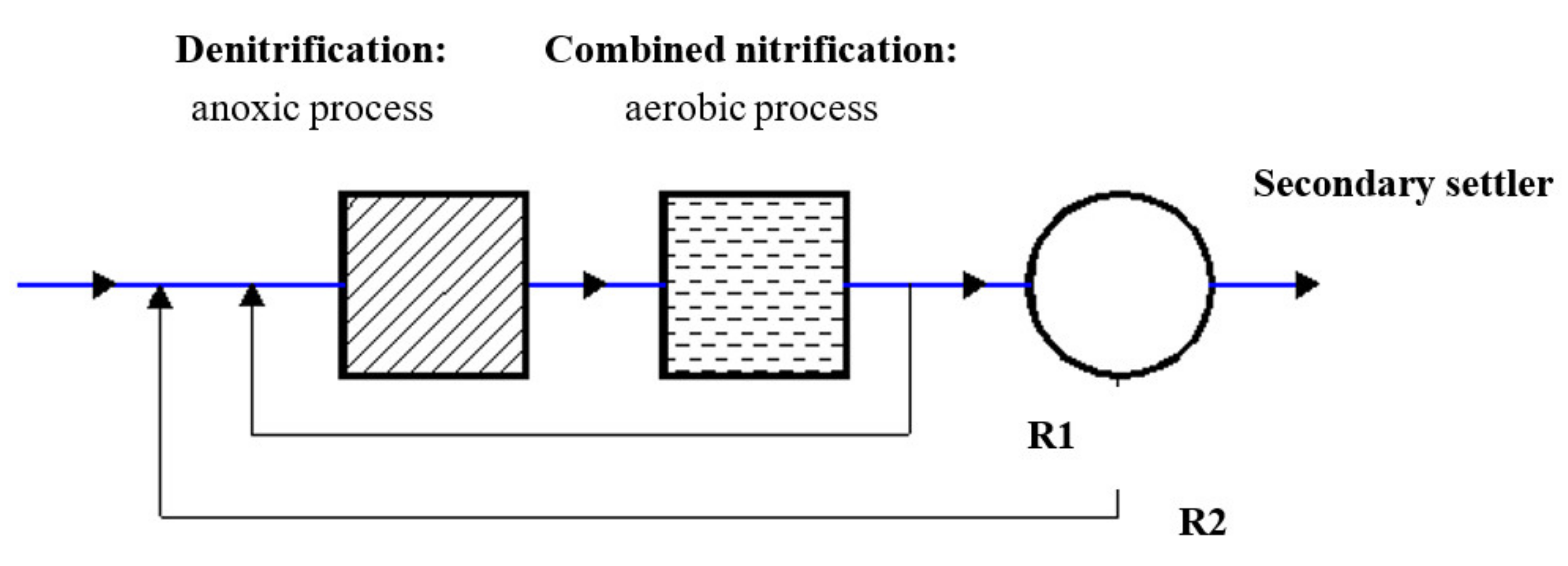
2.1. System Layout
2.2. Calibration and Validation Procedure
3. Results and Discussion
3.1. Sensitivity Analysis
3.2. Energy Analysis
4. Conclusions
Author Contributions
Funding
Conflicts of Interest
Appendix A
Appendix A.1. System Model

| Parameter | Description | Unit | |
|---|---|---|---|
| 1 | SI | Soluble inert organic matter: consists of organic compounds that do not take part in the wastewater treatment processes | mgCODl−3 |
| 2 | SS | Readily biodegradable substrate: simple organic carbon compounds that provide energy to heterotrophic bacteria | mgCODl−3 |
| 3 | XI | Particulate inert organic matter: undissolved organic particles such as soil organic matter or other particulates isolated by sieving or filtration | mgCODl−3 |
| 4 | XS | Slowly biodegradable substrate: consists of relatively complex compounds that must be hydrolysed to simple compounds by extracellular enzymes in order to be assimilated by microorganisms | mgCODl−3 |
| 5 | XBH | Active heterotrophic biomass: microorganisms using organic carbon for the formation of new biomass | mgCODl−3 |
| 6 | XBA | Active autotrophic biomass: microorganisms using carbon from carbon dioxide for the formation of new biomass | mgCODl−3 |
| 7 | XP | Particulate products arising from biomass decay: products which are inert to further biological attack after the decay of the biomass | mgCODl−3 |
| 8 | SO | Oxygen: the oxygen concentration for the biological process | mgl−3 |
| 9 | SNO | Nitrate and nitrite nitrogen: products obtained by autotrophic bacteria in aerobic condition and removed by heterotrophic bacteria in anoxic condition | mgNl−3 |
| 10 | SNH | NH4++ NH3 nitrogen: the soluble ammonia nitrogen, assumed to be the sum of the ionized (ammonium, NH4+) and un-ionized form (ammonia, NH3) | mgNl−3 |
| 11 | SND | Soluble biodegradable organic nitrogen: products formed by the hydrolysis of particular organic nitrogen by ammonification | mgNl−3 |
| 12 | XND | Particulate biodegradable organic nitrogen: products generated from decay of autotrophic and heterotrophic bacteria | mgNl−3 |
| 13 | Salk | Alkalinity | mol m−3 |
| Process, j | Component, i | |||||||||||||
|---|---|---|---|---|---|---|---|---|---|---|---|---|---|---|
| 1 | 2 | 3 | 4 | 5 | 6 | 7 | 8 | 9 | 10 | 11 | 12 | 13 | Process Rate | |
| SI | SS | XI | XS | XBH | XBA | XP | SO | SNO | SNH | SND | XND | Salk | ρj | |
| 1. Aerobic growth of heterotrophs | 1 | |||||||||||||
| 2. Anoxic growth of heterotrophs | 1 | |||||||||||||
| 3. Aerobic growth of autotrophs | 1 | |||||||||||||
| 4. Decay of heterotrophs | 1-fP | −1 | fP | bHXB,H | ||||||||||
| 5. Decay of autotrophs | −1 | baXB,A | ||||||||||||
| 6. Ammonification of soluble nitrogen | 1 | −1 | kaSNDXB,H | |||||||||||
| 7. Hydrolysis of entrapped organics | 1 | −1 | ||||||||||||
| 8. Hydrolysis of entrappedorganic nitrogen | 1 | −1 | ρ7(XND/XS) | |||||||||||
- H = the maximum heterotrophic growth rate, equal to 4.0 (day−1).
- KS = the saturation (heterotrophic growth), equal to 10.0 (g COD m−3).
- KO,H = the half saturation (heterotrophic oxygen), equal to 0.2 (g O2 m−3).
- KNO = the half saturation (nitrate), equal to 0.5 (g NO3-Nm−3).
- bH = the heterotrophic decay rate, equal to 0.3 (day−1).
- ηg = the anoxic growth rate correction factor, equal to 0.8 (-).
- ηh = the anoxic hydrolysis rate correction factor, equal to 0.8 (-).
- kh = the maximum specific hydrolysis rate, equal to 3.0 (g, slowly biodegradable COD (g XBH COD day)−1).
- KX = the half saturation (hydrolysis), equal to 0.1 (g, slowly biodegradable COD (g XBH COD)−1).
- A = the maximum autotrophic growth rate, equal to 0.5 (day−1).
- KNH = the half saturation (auto: growth), equal to 1.0 (g NH3-Nm−3).
- KOA = the half saturation (auto: oxygen), equal to 0.4 (g O2 m−3).
- bA = the autotrophic decay rate, equal to 0.05 (day−1).
- ka = the ammonification rate, equal to 0.05 (m3 COD (g day)−1).
Appendix A.2. Aeration Energy Demand Evaluation
References
- Salgot, M.; Folch, M. Wastewater treatment and water reuse. Curr. Opin. Environ. Sci. Health 2018, 2, 64–74. [Google Scholar] [CrossRef]
- Filipe, J.; Bessa, R.J.; Reis, M.; Alves, R.; Póvoa, P. Data-driven predictive energy optimization in a wastewater pumping station. Appl. Energy 2019, 252, 113423. [Google Scholar] [CrossRef] [Green Version]
- Longo, S.; Mirkod’Antoni, B.; Bongards, M.; Chaparro, A.; Cronrath, A.; Fatone, F.; Lema, J.M.; Mauricio-Iglesias, M.; Soares, A.; Hospido, A. Monitoring and diagnosis of energy consumption in wastewater treatment plants. A state of the art and proposals for improvement. Appl. Energy 2016, 179, 1251–1268. [Google Scholar] [CrossRef]
- Zhang, Z.; Kusiak, A.; Zeng, Y.; Wei, X. Modeling and optimization of a wastewater pumping system with data-mining methods. Appl. Energy 2016, 164, 303–311. [Google Scholar] [CrossRef]
- Guven, H.; Dereli, R.K.; Ozgun, H.; Ersahin, M.E.; Ozturk, I. Towards sustainable and energy efficient municipal wastewater treatment by up-concentration of organics. Prog. Energy Combust. Sci. 2019, 70, 145–168. [Google Scholar] [CrossRef]
- Shen, Y.; Linville, J.L.; Urgun-Demirtas, M.; Mintz, M.M.; Snyder, S.W. An overview of biogas production and utilization at full-scale wastewater treatment plants (WWTPs) in the United States: Challenges and opportunities towards energy-neutral WWTPs. Renew. Sustain. Energy Rev. 2015, 50, 346–362. [Google Scholar] [CrossRef] [Green Version]
- Wang, J.; You, S.; Zong, Y.; Træholt, C.; Dong, Z.Y.; Zhou, Y. Flexibility of combined heat and power plants: A review of technologies and operation strategies. Appl. Energy 2019, 252, 113445. [Google Scholar] [CrossRef]
- Salman, C.A.; Naqvi, M.; Thorin, E.; Yan, J. Impact of retrofitting existing combined heat and power plant with polygeneration of biomethane: A comparative techno-economic analysis of integrating different gasifiers. Energy Convers. Manag. 2017, 152, 250–265. [Google Scholar] [CrossRef]
- Picardo, A.; Soltero, V.M.; Peralta, M.E.; Chacartegui, R. District heating based on biogas from wastewater treatment plant. Energy 2019, 180, 649–664. [Google Scholar] [CrossRef]
- Calise, F.; Cappiello, F.L.; Dentice d’Accadia, M.; Infante, A.; Vicidomini, M. Modeling of the Anaerobic Digestion of Organic Wastes: Integration of Heat Transfer and Biochemical Aspects. Energies 2020, 13, 2702. [Google Scholar] [CrossRef]
- Di Fraia, S.; Macaluso, A.; Massarotti, N.; Vanoli, L. Energy, exergy and economic analysis of a novel geothermal energy system for wastewater and sludge treatment. Energy Convers. Manag. 2019, 195, 533–547. [Google Scholar] [CrossRef]
- Nelson, M.I.; Sidhu, H.S.; Watt, S.; Hai, F.I. Performance analysis of the activated sludge model (number 1). Food Bioprod. Process. 2019, 116, 41–53. [Google Scholar] [CrossRef]
- Henze, M.; Grady, C.P.L., Jr.; Gujer, W.; Marais, G.V.R.; Matsuo, T. A general model for single-sludge wastewater treatment systems. Water Res. 1987, 21, 505–515. [Google Scholar] [CrossRef] [Green Version]
- Hauduc, H.; Rieger, L.; Oehmen, A.; van Loosdrecht, M.C.M.; Comeau, Y.; Héduit, A.; Vanrolleghem, P.A.; Gillot, S. Critical review of activated sludge modeling: State of process knowledge, modeling concepts, and limitations. Biotechnol. Bioeng. 2013, 110, 24–46. [Google Scholar] [CrossRef] [PubMed]
- Moretti, C.J.; Jahan, K.; Schmit, K.H.; Debik, E.; Mahendraker, V. Activated Sludge and Other Aerobic Suspended Culture Processes. Water 2011, 3, 806–818. [Google Scholar] [CrossRef]
- Available online: https://pdfs.semanticscholar.org/b076/822899ab977bd49e271e51ae6fa8ec9ad951.pdf (accessed on 30 July 2020).
- Available online: https://op.europa.eu/en/publication-detail/-/publication/8448ef88-37dd-4d1a-823f-3143e7902429 (accessed on 30 July 2020).
- The European Co-Operation in the Field of Scient. ific and Technical Research, Action 624: Optimal Management of Wastewater SystemsCOST Action 624 Website. Available online: http://www.ensic.inpl-nancy.fr/COSTWWTP (accessed on 30 July 2020).
- Asadi, A.; Yang, K.; Mejabi, B. Wastewater treatment aeration process optimization: A data mining approach. J. Environ. Manag. 2017, 203, 630–639. [Google Scholar] [CrossRef] [PubMed]
- Sheridan, C.; Petersen, J.; Rohwer, J. Technical note on modifying the Arrhenius equation to compensate for temperature changes for reactions within biological systems. Water SA 2012, 38, 149–152. [Google Scholar] [CrossRef] [Green Version]
- Henze, M.; Gujer, W.; Mino, T.; van Loosdrecht, M.C.M. Activated Sludge Models ASM1, ASM2, ASM2d and ASM3; IWA Publishing: London, UK, 2000. [Google Scholar]
- Takacs, I.; Patry, G.G.; Nolasco, D. A dynamic model of the clarification-thickening process. Wat. Res. 1991, 25, 1263–1271. [Google Scholar] [CrossRef]
- Alex, J.; Benedetti, L.; Copp, J.; Gernaey, K.V.; Jeppsson, U.; Nopens, I.; Pons, M.N.; Rieger, L.; Rosen, C.; Steyer, J.P.; et al. Benchmark Simulation Model no 1 (BSM1). Department of Industrial Electrical Engineering and Automation, Lund University. Available online: https://www.iea.lth.se/publications/Reports/LTH-IEA-7229.pdf (accessed on 30 July 2020).


| Concentration of | Inflow | Anoxic Tank 1 Initial | Anoxic Tank 2 Initial | Aeration Tank 1 Initial | Aeration Tank 2 Initial | Aeration Tank 3 Initial |
|---|---|---|---|---|---|---|
| (gm−3) | ||||||
| Readily biodegradable substrate | 69.500 | 3.732 | 2.061 | 1.454 | 1.226 | 1.067 |
| Soluble inert organic | 30.000 | 30.000 | 30.000 | 30.000 | 30.000 | 30.000 |
| Particulate inert organic matter | 51.200 | 814.301 | 813.912 | 813.393 | 812.874 | 812.354 |
| Slowly biodegradable substrate | 202.320 | 83.073 | 81.401 | 68.023 | 57.215 | 49.092 |
| Active heterotrophic biomass | 28.170 | 2085.021 | 2083.728 | 2088.379 | 2091.048 | 2091.868 |
| Active autotrophic biomass | 0 | 69.621 | 69.535 | 69.839 | 70.152 | 70.382 |
| Particulate products arising from biomass decay | 0 | 227.672 | 228.044 | 228.540 | 229.037 | 229.534 |
| Dissolved oxygen | 0 | 0.012 | 0.000 | 2.938 | 3.752 | 1.076 |
| Nitrate and nitrite nitrogen | 0 | 1.649 | 0.543 | 2.177 | 3.881 | 5.089 |
| Ammonia nitrogen | 31.560 | 17.672 | 18.135 | 16.549 | 15.029 | 13.901 |
| Soluble biodegradable organic nitrogen | 6.950 | 1.319 | 0.859 | 0.914 | 0.881 | 0.808 |
| Particulate biodegradable organic nitrogen | 10.590 | 5.234 | 5.235 | 4.485 | 3.872 | 3.410 |
| Concentration of | Results Obtained | Biowin [4] | Simba [19] | Stoat [5] |
|---|---|---|---|---|
| (gm−3) | ||||
| Readily biodegradable substrate | 0.890 | 0.890 | 0.889 | 0.900 |
| Soluble inert organic | 30.000 | 30.000 | 30.000 | 30.000 |
| Particulate inert organic matter | 4.392 | 4.270 | 4.392 | 6.100 |
| Slowly biodegradable substrate | 0.188 | 0.210 | 0.188 | 0.140 |
| Active heterotrophic biomass | 9.782 | 9.510 | 9.782 | 6.600 |
| Active autotrophic biomass | 0.573 | 0.560 | 0.573 | 0.400 |
| Particulate products arising from biomass decay | 1.728 | 1.680 | 1.728 | - |
| Dissolved oxygen | 0.491 | 0.500 | 0.491 | 0.500 |
| Nitrate and nitrite nitrogen | 10.415 | 10.450 | 10.415 | 10.400 |
| Ammonia nitrogen | 1.733 | 1.740 | 1.733 | 1.700 |
| Soluble biodegradable organic nitrogen | 0.688 | 0.690 | 0.688 | 0.700 |
| Particulate biodegradable organic nitrogen | 0.013 | 0.010 | 0.013 | 0.000 |
| TSS Concentrations Along the Settler Height | Results Obtained | Biowin [4] | Simba [19] | Stoat [5] |
|---|---|---|---|---|
| (gSSm−3) | ||||
| Layer 1 (effluent source) | 12.497 | 12.170 | 12.500 | 12.500 |
| Layer 2 | 18.113 | n/a | 18.110 | 18.100 |
| Layer 3 | 29.540 | n/a | 29.540 | 29.500 |
| Layer 4 | 68.978 | n/a | 68.980 | 68.900 |
| Layer 5 | 356.075 | n/a | 356.070 | 356.100 |
| Layer 6 | 356.075 | n/a | 356.070 | 356.100 |
| Layer 7 | 356.075 | n/a | 356.070 | 356.100 |
| Layer 8 | 356.075 | n/a | 356.070 | 356.100 |
| Layer 9 | 356.075 | n/a | 356.070 | 356.100 |
| Layer 10 (activated sludge source) | 6393.984 | 6406.030 | 6393.980 | 6394.100 |
| Volume Tank 1, 2 (m3) | Volume Tank 3, 4, 5 (m3) | kLa (day−1) | EQI (kg pollutions d−1) | Electric Demand (kW) | Primary Energy Consumption (MWh/y) | ΔPE (%) | CO2 (tCO2/y) | ΔCO2 (%) |
|---|---|---|---|---|---|---|---|---|
| 1000 | 1333 | 240 | 5508 | 185 | 3520 | - | 782 | - |
| 1000 | 1666 | 144 | 5109 | 161 | 3061 | 13.0 | 680 | 13.0 |
| 1250 | 1666 | 144 | 4941 | 163 | 3105 | 11.8 | 690 | 11.8 |
| 1250 | 2000 | 120 | 4546 | 165 | 3145 | 10.7 | 699 | 10.6 |
| 1500 | 2000 | 108 | 4968 | 163 | 3103 | 11.8 | 689 | 11.9 |
| 2000 | 2666 | 84 | 4129 | 175 | 3339 | 5.1 | 742 | 5.1 |
© 2020 by the authors. Licensee MDPI, Basel, Switzerland. This article is an open access article distributed under the terms and conditions of the Creative Commons Attribution (CC BY) license (http://creativecommons.org/licenses/by/4.0/).
Share and Cite
Calise, F.; Eicker, U.; Schumacher, J.; Vicidomini, M. Wastewater Treatment Plant: Modelling and Validation of an Activated Sludge Process. Energies 2020, 13, 3925. https://doi.org/10.3390/en13153925
Calise F, Eicker U, Schumacher J, Vicidomini M. Wastewater Treatment Plant: Modelling and Validation of an Activated Sludge Process. Energies. 2020; 13(15):3925. https://doi.org/10.3390/en13153925
Chicago/Turabian StyleCalise, Francesco, Ursula Eicker, Juergen Schumacher, and Maria Vicidomini. 2020. "Wastewater Treatment Plant: Modelling and Validation of an Activated Sludge Process" Energies 13, no. 15: 3925. https://doi.org/10.3390/en13153925