Article

Energy Intensity and Long- and Short-Term Efficiency in US Manufacturing Industry

by
Oleg Badunenko
1,† and
Subal C. Kumbhakar
2,3,*,†
1
Department of Economics and Finance, College of Business, Arts and Social Sciences, Brunel University London, Uxbridge UB8 3PH, UK
2
Department of Economics, State University of New York at Binghamton, Binghamton, NY 13902-6000, USA
3
Department of Innovation, Management and Marketing, University of Stavanger Business School, University of Stavanger, N-4036 Stavanger, Norway
*
Author to whom correspondence should be addressed.
These authors contributed equally to this work.
Energies 2020, 13(15), 3954; https://doi.org/10.3390/en13153954
Submission received: 22 June 2020 / Revised: 16 July 2020 / Accepted: 27 July 2020 / Published: 1 August 2020
(This article belongs to the Collection Energy Use Efficiency)

Abstract

:
We analyze energy use efficiency of manufacturing industries in US manufacturing over five decades from 1960 to 2011. We apply a 4-component stochastic frontier model, which allows disentangling efficiency into a short- and long-term efficiency as well as accounting for industry heterogeneity. The data come from NBER-CES Manufacturing Industry Database. We find that relative to decade-specific frontiers, the overall efficiency of manufacturing industries, which is a product of transient and persistent efficiencies has deteriorated greatly in the 1970s and rebounded only in the 2000s. The industries are very efficient in the short-term and this has not changed over five decades. The high level of overall inefficiency is almost completely due to the structural inefficiency which can be explained by what is referred to as the “energy paradox”. Finally, higher energy-intensive industries perform worse in terms of energy use efficiency than their low energy-intensity counterparts.

1. Introduction

According to the U.S. Energy Information Administration, manufacturing industries in the US consume about a third of total energy consumed (see also [1]). (https://www.eia.gov/consumption/) The analysis of energy demand for manufacturing has therefore important implications for energy policy, where energy efficiency and savings is an important agenda (see, e.g., [2]). Additionally, improving energy use efficiency seems to be a natural way to mitigate climate change (see, e.g., [3]). If manufacturing industries are not efficient, it puts strains on the whole economy in general and energy producers and distributors in particular. This is especially true for the energy-intensive industries where energy consumption relative to its output is large.
For a long time, a lot of effort has been made to develop energy-efficient technologies, not only to lessen environmental damage but also to bring down the monetary cost of production. However, Reference [4] identify and discuss the wide-spread “energy-paradox”, whereby energy-efficient technologies, that would have paid-off, are in reality not adopted. The authors of [5] find that the adoption of energy-efficient technologies may be boosted by involving managers, who are in a position close to operations. The existence of the “energy-paradox” may indicate that the industry remains inefficient. Indeed, Reference [6] find that the mean plant-level efficiency in the United States over the time-period 1987–2012 ranges from 33% to 86% for plants in various manufacturing industries.
Such huge inefficiencies are a matter of concern. Enormous financial savings could have been achieved if manufacturing firms were more efficient. The performance of manufacturing in terms of energy use is heterogeneous both in time and cross-sectional dimensions. One common factor influencing energy consumption is the price of energy. The authors of [7] confirm that the biggest determinant of energy intensity is the price of electricity. The cross-sectional variation is further determined by technology, i.e., some industries require more energy than others. The time variation has many determinants. Most important is probably the change in macroeconomic conditions. The beginning of the 1970s was marked by the oil prices, which had a detrimental effect on costs related to energy in manufacturing. It was an expectation that there should have been a surge in adopting the new energy-saving technologies which would eventually improve energy efficiencies. However, Reference [8] finds that the energy consumption did not rebound quickly implying that the response to a decline in real energy prices was slow.
In this paper, we investigate the energy use efficiency of US manufacturing from 1958 to 2011. More specifically, we conduct an analysis at an aggregated level, where the unit of observation is defined as NBER 6-digit NAICS (see [9]). We split the whole time period into five decades and assume a decade-specific technology. We define energy intensity as energy demand per measure of economic activity (see, e.g., [10]). In each decade, we consider 10 percent the most and least energy-intensive industries. Further, following [11], we decompose overall inefficiency into persistent or structural and transient inefficiencies. This has an advantage over for example [3] or [6] since we can identify if efficiency can be improved with relatively small effort, or structural approach is required. We find a significant drop in energy use efficiency in the 1970s, which has probably been caused by the oil crisis. The return to the pre-1970s levels was reached only in the 2000s, which is in agreement with slow rebound estimates of energy consumption (see, e.g., [8]). Remarkably, such low levels of overall energy use efficiency owing to very low levels of structural inefficiency that cannot be managed with ease. This finding goes in unison with the “energy-paradox” (see [4]). Finally, higher energy-intensive industries are characterized by lower levels of energy use efficiency than low-intensive counterparts.
The paper is organized as follows. Section 3 introduces models that are used to measure energy use efficiency and 4-component stochastic frontier model that accounts for heterogeneity and splits overall inefficiency into persistent and transient components. Section 4 describes data and variable construction. Empirical results are presented and discussed in Section 5. Section 6 concludes.

2. Literature Review

Analysis of the energy use efficiency is interesting from both academic and business perspective. More efficient use, especially by energy-intensive industries, would result in lower demand for energy as well as output (see, e.g., [12]). Examining efficiency estimates could also complement accounting for rebound effects ([13]) when making energy consumption forecasts. Energy subsidies could also be inappropriately targeted to support highly inefficient producers if inefficiency measurement is improper (see, e.g., [14]). Here we provide a brief review of methods used in measuring energy and technical or cost efficiency.
Depending on the available data, measurement of technical efficiency can be done by using either stochastic frontier (SF) methods (see [15]) or data envelopment analysis (DEA) approach (see [16]). For a cross-sectional data with fewer observations, one can opt for DEA to estimate the benchmark and then measure inefficiency as a deviation from the benchmark. SF in contrast defines the benchmark accommodating stochastic noise and decomposes the composed error (sum of noise and inefficiency) into inefficiency and statistical noise. The noise can be both positive and negative and can be seen as positive and negative shocks to the production process. In the panel-data context, there are different possibilities to decompose the composed error term. One way is to allow inefficiency to be persistent and hence time-invariant. This approach is referred to as the first-generation panel-data SF modeling. The second-generation SF models assume that the inefficiency is time-varying. The first and second-generation models assume an error term (the deviation from the frontier) that has two components. Applying DEA to a panel data would be comparable to a second-generation SF model, which would produce time-varying efficiency estimates without accounting for possible noise. The third-generation SF model considers an error term with three components. The two components are time and firm-specific, i.e., statistical noise and time-varying inefficiency. The third component is time constant. The authors of [17,18,19,20] propose to treat it as time-invariant inefficiency. The authors of [21] assume it is an individual effect or firm heterogeneity. Thus, Kumbhakar and co-authors model two types of inefficiency (persistent and transient) ignoring heterogeneity, while Greene models transient inefficiency and heterogeneity ignoring persistent inefficiency. The fourth-generation class of SF models is originally introduced by [22] and accounts for both types of inefficiency as well as heterogeneity. Incidentally, the fourth-generation SF models are also known as the 4-component SF models.
Traditionally, energy efficiency measurement is contemplated in terms of energy intensity. However, it is argued that other measures should also be considered, for example DEA ([23]). This was one of the first studies to consider the production theory framework as a base for energy efficiency measurement. The authors of [23] employ DEA for the manufacturing sector constructed by the U.S. Bureau of Labor Statistics (BLS). She finds quite high efficiency scores for aggregate manufacturing for the 1970–2001 time period. Recall, however, that DEA does not account for heterogeneity or persistent efficiency akin to the second generation SF models, which can be seen as a disadvantage of using DEA. Furthermore, she finds higher efficiency scores towards the end of the sample. But because she used an intertemporal frontier approach, she could not distinguish whether this is attributed to technical progress or not. This can be viewed as the second disadvantage of using DEA when panel data are available. Many other studies have used DEA to analyze energy efficiency. The authors of [24], for example, investigate the energy efficiency of the Indian manufacturing sector for the 1998–2004 time period. The authors of [25] apply DEA to measure economy-wide energy efficiency using aggregated data on the OECD countries. The authors of [26] investigate energy use efficiency of canola production in Iran. See the review of [27] for other studies that employ DEA.
SFA has also been used to measure energy efficiency and efficiency in the energy sector. The authors of [28,29] were the first to advocate using SFA to estimate efficiency in manufacturing sectors. However, he did not go beyond a cross-sectional analysis. The authors of [30] use the second-generation SF model to measure energy efficiency of different states in the US residential sector. The authors of [31] investigate energy efficiency in the automotive manufacturing sector using plant-level data. The authors again use the second generation model. The authors of [32] are the first to use the third generation SF model to analyze the efficiency of the Swiss electricity distribution sector. The authors of [33] used the fourth-generation model to aggregate frontier energy demand model and estimate economy-wide persistent and transient energy efficiency in the US. The authors confirm the findings and arguments of [23] that energy intensity is not a good indicator of energy efficiency. The authors of [33] as well as [34] emphasize the importance of accounting for heterogeneity as well as estimating two types of inefficiency. This is the approach, which we apply for the first time to this type of data using three different models. Our models are described in the next section.

3. Methodology

3.1. Models

In this paper, we apply three different models to investigate energy use efficiency. In all models, we assume that the production technology consists of one output Y and a vector of four inputs X = ( L , K , N E M , E ) , where L is the labor, K is the capital stock, N E M is the non-energy materials, and E is the energy. The production technology using multiple outputs (transformation function), can be written, in implicit form as,
A F ( Y , X ) = 1 .
If the manufacturing process does not experience production shocks, A = 1 , and F ( Y , X ) = 1 . However, since both positive and negative shows hit the production, the transformation function is made stochastic by setting A = exp ( v ) , v can be both positive and negative. Besides, if inputs are not used with 100% efficiency, the transformation function in (1) can be expressed as
A F ( Y , θ X ; β ) = 1 ,
where θ < 1 is the input technical efficiency (defined as the ratio of minimum of each input required and actual amount used) and β is the set of the technology parameters of the function F . Since the transformation function is homogeneous of degree 1 in inputs (see [35]), so we can rewrite (2) as
A F ( Y , λ θ X ; β ) = λ , λ > 0 .
Further, we can set λ = ( E θ ) 1 , where E is the energy input. Note that any other input could have been chosen to be in place of E. Then (3) becomes
X 1 1 θ 1 = f ( Y , X ˜ E ; β ) exp v ,
where X ˜ E = ( L / E , K / E , N E M / E ) . Taking logs of both sides of (4) and denoting u = log θ 0 , we obtain (Model 1)
log E = log f ( Y , X ˜ E ; β ) + v u .
The stochastic frontier (SF) formulation in (5) is known as the input distance function formulation, where u is input oriented inefficiency, which measures percentage (when multiplied by 100) over-use of all the inputs. For small values of u, e u 1 u . That is, technical efficiency is 1 minus technical inefficiency. It is important to keep this relationship in mind because we switch from one to the other quite frequently. Technical efficiency in this model refers to the efficiency of all inputs including energy. That is, in this model, inefficiency, u, is interpreted as over-use of all the all inputs, including energy, at the same rate. The other two models focus exclusively on energy-use efficiency. Before we explain how u can be estimated, we introduce two other approaches.
The transformation function can also be written as a factor requirement function (see, e.g., [36]). Since the focus is on energy use, we can express the technology in terms of E, and write it as,
E = G ( Y , X E ) ,
where X E = ( L , K , N E M ) . Again, assuming that both positive and negative shocks v can influence energy requirement and positing that energy is not used 100% efficiently used, we can rewrite (6) as
E = g ( Y , X E ; γ ) exp v exp u ,
where γ is the vector of parameters of the energy requirement function, v is a symmetric error term and u is the energy use inefficiency. Taking to logs of both sides of the (7) gives us the energy requirement function with inefficiency, viz., (Model 2)
log E = log g ( Y , X E ; γ ) + v + u .
This approach was, for example, applied by [6,29] to plant-level data using the second-generation SF model. Note that (8) has a stochastic cost function type formulation. Any inefficiency in the use of energy will increase cost.
Finally, in our last model we recognize endogeneity of output Y. That is, we assume profit maximizing behavior to derive the energy demand function
E = H ( w , X E ) ,
where w = w E / p , w E is the energy price and p is the output price. Similar to the factor requirement function, we can obtain energy use inefficiency from the demand function (Model 3)
log E = log h ( w , X E ; δ ) + v + u ,
where δ is the vector of parameters of the energy demand function, v is a symmetric error term and u is the energy use inefficiency.
The difference between (5) and (10) is that in the latter energy input is chosen optimally by maximizing profit. In (5) energy overuse treats all other inputs as given. That is, inefficiency in this model shows by how much energy is overused to produce a given level of output and all other inputs. On the other hand, inefficiency in (10) comes from excess use of energy when all other inputs and output are chosen optimally instead of taking them as exogenously given. From econometric estimation point of view this means Y and X E are exogenous in Model 2, whereas they are endogenous in Model 3.
In the next sub-section we examine all three models in more detail in the light of panel stochastic frontier framework. In particular, we add firm-heterogeneity and decompose inefficiency into persistent and transient components.

3.2. Stochastic Frontier Approach with Panel Data

The stochastic production frontier function approach was introduced for cross-sectional data independently by [37,38]. This is expressed as
log q i = r ( X i ; ω ) + v i u i ,
where r ( · ) is the technology (namely, the production function in logarithmic form), q i is an output, X i is a vector of inputs (in log) for a production unit i, ω is a vector of parameters that define the technology, v i is the usual error/noise term, and u i 0 is the inefficiency. In this model, the data are cross-sectional and hence error components v i and u i represents cross-sectional shocks to the production and production unit-specific inefficiency. When panel data are available, shocks and inefficiency can be both time-constant and time-varying. The authors of [22,39,40] were first to recognize this and formulated the following 4-component stochastic frontier model for panel data. We use this framework for our Model 1, and write it as:
log q i t = r ( X i t , t r e n d ; ω ) + v 0 i u 0 i + v i t u i t ,
where t is a time period in which a production unit i is observed. In (12) we have two additional terms compared to (11). More specifically, v i t is the usual symmetric error term, v 0 i is an individual (production unit) effect also known to represent individual production shock (or heterogeneity), u 0 i 0 is the persistent or structural time-invariant inefficiency, and finally u i t 0 is the transient or short-term time-varying inefficiency. Thus, the overall inefficiency is the sum of persistent and transient inefficiency and overall efficiency T E o v e r a l l is decomposed into persistent T E p e r s i s t e n t and transient T E t r a n s i e n t , i.e.,
T E o v e r a l l = T E p e r s i s t e n t × T E t r a n s i e n t
Note that persistent and transient efficiency ( T E p e r s i s t e n t and T E t r a n s i e n t ) are defined as e u 0 i and e u i t , respectively. The originally proposed model assumed all 4 components to be random and homoskedastic. This model did not include the determinants of inefficiency. In our analysis, we will use the [11] model that introduces determinants of both types of inefficiency in (12).
To estimate parameters ω in (12), we assume that v i t N 0 , σ v i t , v 0 i N 0 , σ v 0 i , u i t N + 0 , σ u i t , and u 0 i N + 0 , σ u 0 i , where N + means the positive part of the zero mean normal distribution, making u i t and u 0 i half-normally distributed. We assume that both noise v i t and individual effects v 0 i are homoskedastic, so that σ v i t = σ v and σ v 0 i = σ v 0 . We introduce determinants of time-varying inefficiency via the pre-truncated variance of u i t . More specifically, we assume
σ u i t 2 = exp z u i t ψ u , i = 1 , , n , t = 1 , , T i ,
where z u i t denotes the vector of covariates that explain time-varying inefficiency. Since u i t is half-normal, E ( u i t ) = ( 2 / π ) σ u i t = ( 2 / π ) exp 1 2 z u i t ψ u , and therefore, anything that affects σ u i t also affects time-varying inefficiency. The determinants of persistent inefficiency can be modeled similarly. However, because the data-set does not provide natural determinants of the persistent inefficiency, we leave it homoskedastic, i.e., σ u 0 i = σ u 0 .
The parameters ω , as well as variances of the 4 components and their determinants, can be estimated by the single stage maximum simulated likelihood (MSL) method (see Appendix B and [11] for details of the estimation procedure). We follow [39] to calculate the persistent and transient efficiencies. The overall efficiency is then calculated as the product of the persistent and transient efficiencies.
We add firm-heterogeneity and decompose inefficiency into persistent and transient inefficiency in the same way as in Model 1, for both Models 2 and 3, which are outlined in (8) and (10). After adding these components, the models will look quite similar to (12) mathematically. Because of this, we skip the details and avoid repetitions. However, note that the interpretation of inefficiency in these models are different. In Model 2 inefficiency refers to overuse of energy, given everything else. Consequently, persistent and transient inefficiency in Model 2 decompose energy overuse into a time-invariant and a time-varying components, ceteris paribus. Similar to Model 2, inefficiency in Model 3 described in (10) after adding firm heterogeneity and persistent inefficiency is specifically related to energy overuse. But it does not take other inputs as given, which is what Model 2 does. In Model 3 inputs are chosen optimally, and inefficiency in production is transmitted to overuse of inputs via demand for energy. That is, we focus only on energy by examining the energy demand function.

4. Data

The source of the data we use in this paper is NBER-CES Manufacturing Industry Database, which can be accessed at http://www.nber.org/nberces/. It covers 473 six-digit 1997 NAICS manufacturing industries over 1958–2011. We split our analysis into five decades: 1958–1969 (labeled “the 1960s”), 1970–1979 (labeled “the 1970s”), 1980–1989 (labeled “the 1980s”), 1990–1999 (labeled “the 1990s”), and 2000–2011 (labeled “the 2000s”).
The output Y of an industry is calculated as the difference between the value of industry shipments, which are based on net sales, after discounts and allowances, and the change in end-of-year inventories. The labor L is calculated as P R O D H P A Y / P R O D W , where P R O D H is the number of production worker hours, P A Y is the total payroll, and P R O D W is production workers’ wages. Capital stock K is obtained as the sum of real equipment and real structures. Energy E is the expenditure on purchased fuels and electrical energy. The cost of overall materials M A T C O S T in the database includes delivered cost of raw materials, parts, and supplies put into production or used for repair and maintenance and purchased electric energy and fuels consumed for heat and power and contract work done by others for the plant. The cost excludes the costs of services used, overhead costs, or expenditures related to plant expansion. Because the overall cost of materials includes energy, the non-energy materials, N E M are determined as the difference between overall materials and E. See [9] for more details.
The paper analyzes the differences in energy use efficiency between industries that use relatively little and a lot of energy in their production. We define energy intensity E N _ I N T E N S I T Y as the ratio of the expenditures on purchased fuels and electrical energy E and the value of industry shipments V S H I P , which is the energy cost per unit of sales. The authors of [10], for example, define energy intensity as energy consumption divided by a measure of economic activity. Alternatively, one can define energy intensity as the cost of energy in total costs. We have tried this approach and the correlation coefficient between these two measures of energy intensity was 0.98. So either of them could be used.
Table A1 shows the summary statistics for output and four inputs for 10 percent of the top and bottom energy-intensive manufacturing industries in the respective decade. The criterion to include an industry is that data on it is available for at least 4 years in a decade.

5. Empirical Results

5.1. Change in Energy Intensity of Industries

First, we analyze how energy intensity has evolved in US manufacturing for over the five decades. We concentrate on the top and bottom 10% of the industries in terms of their energy intensity. More specifically, we calculate the 10th and 90th percentile of energy intensity in the 1960s, then we consider industries whose energy intensity is smaller than the 10th percentile and larger than the 90th percentile in the 1960s. Of these industries, we consider only those for which data are available for a period of at least 4 years. Then we repeat this exercise for the other four decades. Table 1 gives a summary statistics of the energy intensity for all industries for the period 1958–2011 as well as by decade and by energy intensity. As we can see, there are industries for which the energy use is negligible. However, some industries consume quite a lot of energy in the production process. All parts of the distribution were increasing up to the 1990s and then started declining.
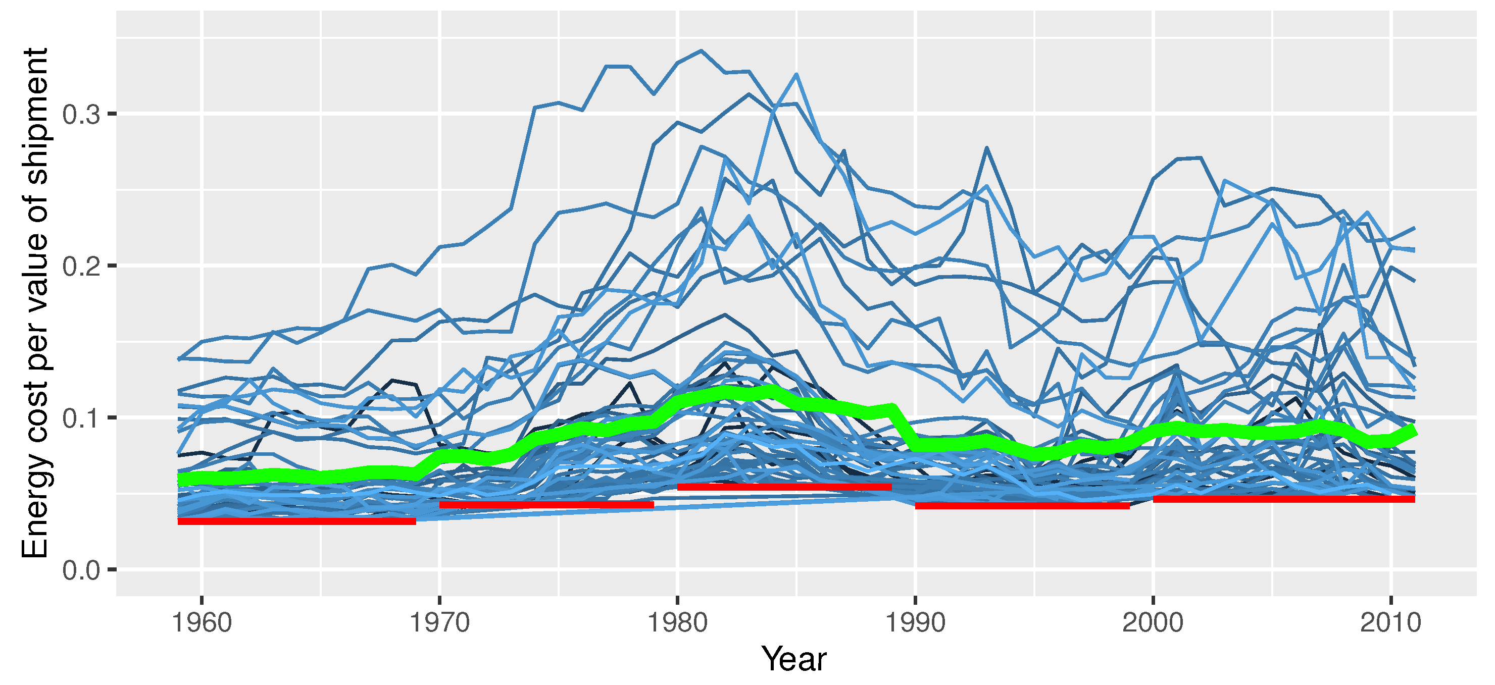
It can be seen that in each decade, the 10th and 90th percentiles are specific for the decade. The industries that satisfy the above procedure are shown in Figure 1 and Figure 2. The red decade-specific horizontal lines show 10th and 90th percentiles for low and high energy-intensive industries, respectively. The bold green solid line shows the mean of energy intensity for these industries.
One conclusion that we can draw from Figure 1 and Figure 2 and Table 1 is that the energy intensity has a shape that is closer to a parabola than a flat line. Whether we are looking at the 10th or the 90th percentile, the energy intensity has been increasing from 1960s through the 1980s and then started to fall in the 1990s and then stalled through the 2000s. One possible explanations can be that energy was abundant and relatively cheap up until 1990s when manufacturers started to consider better and more energy-saving technologies.

5.2. Energy Use Efficiency

In this section, we present the results from three models that are presented in Equations (3), (8) and (10). In all three models, the transient inefficiency is modeled to follow either linear or quadratic trend, that is σ u i t is a function of time in (14). Further, in all three models, we used a translog (log quadratic) specification for the underlying technology. The first model considers energy use inefficiency via an input distance function (IDF). Since inefficiency is radial in the IDF formulation in (3), the energy use efficiency is the same as the efficiency in the use of all other inputs. In the latter two models, inefficiency comes from energy use alone. The difference is that in (10), output can be endogenous, and manufacturing firms are assumed to be profit-maximizing.
The results from models 1, 2, and 3 by decade are presented in Table 2, Table 3 and Table 4. We observe that in all these models, with an exception of the model 3 for the 1990s, all 4 components are statistically significant and thus use of the [11] model is justified. So, the conclusion about appropriateness of using the 4-component model is in line with [33,34]. This means that models that account for only two components such as [41,42,43], or three components such as [21] or [18,19,20] are misspecified and likely to produce wrong results on efficiency. For the 1990s, model 3 could have been estimated using [20] approach.
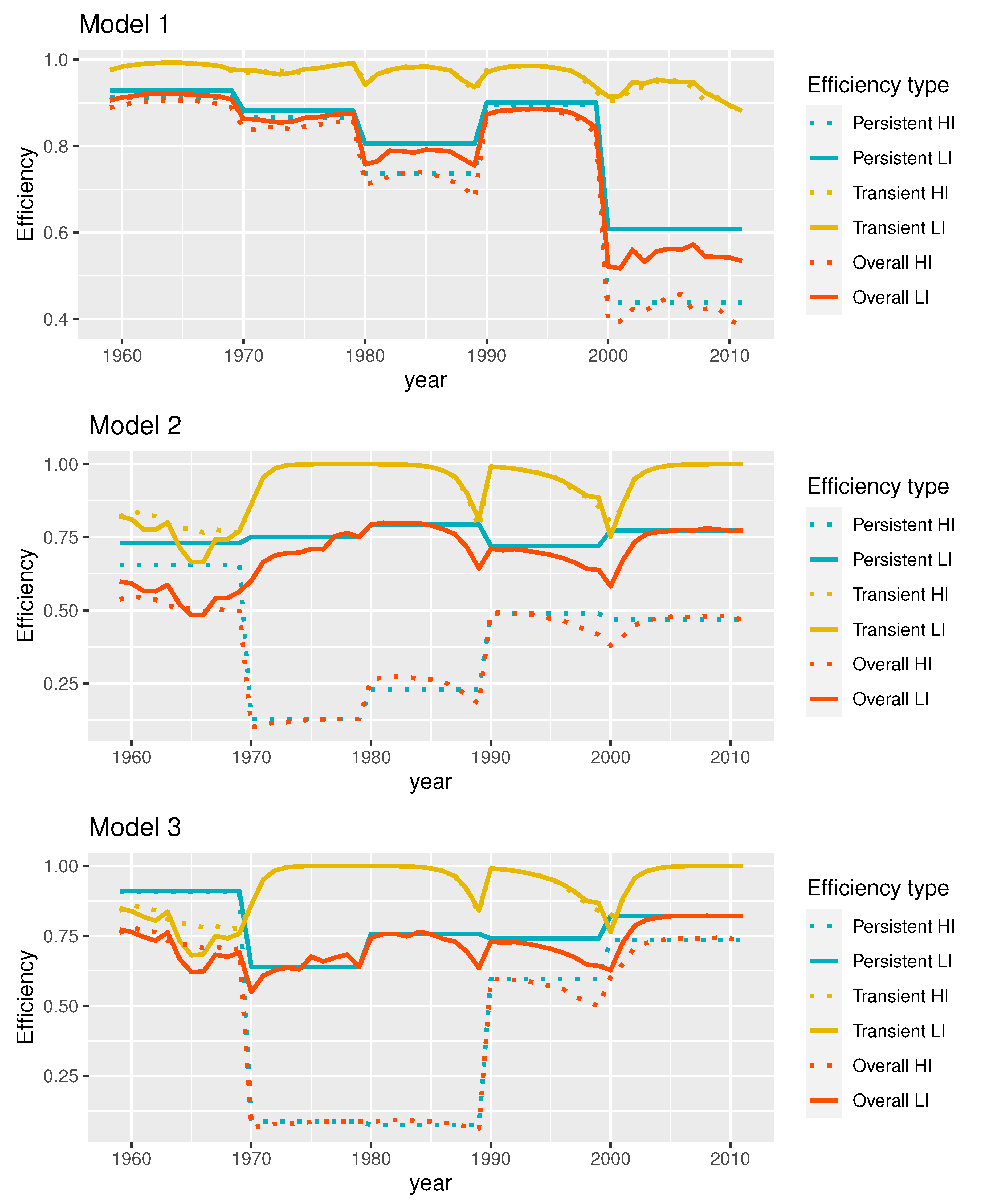
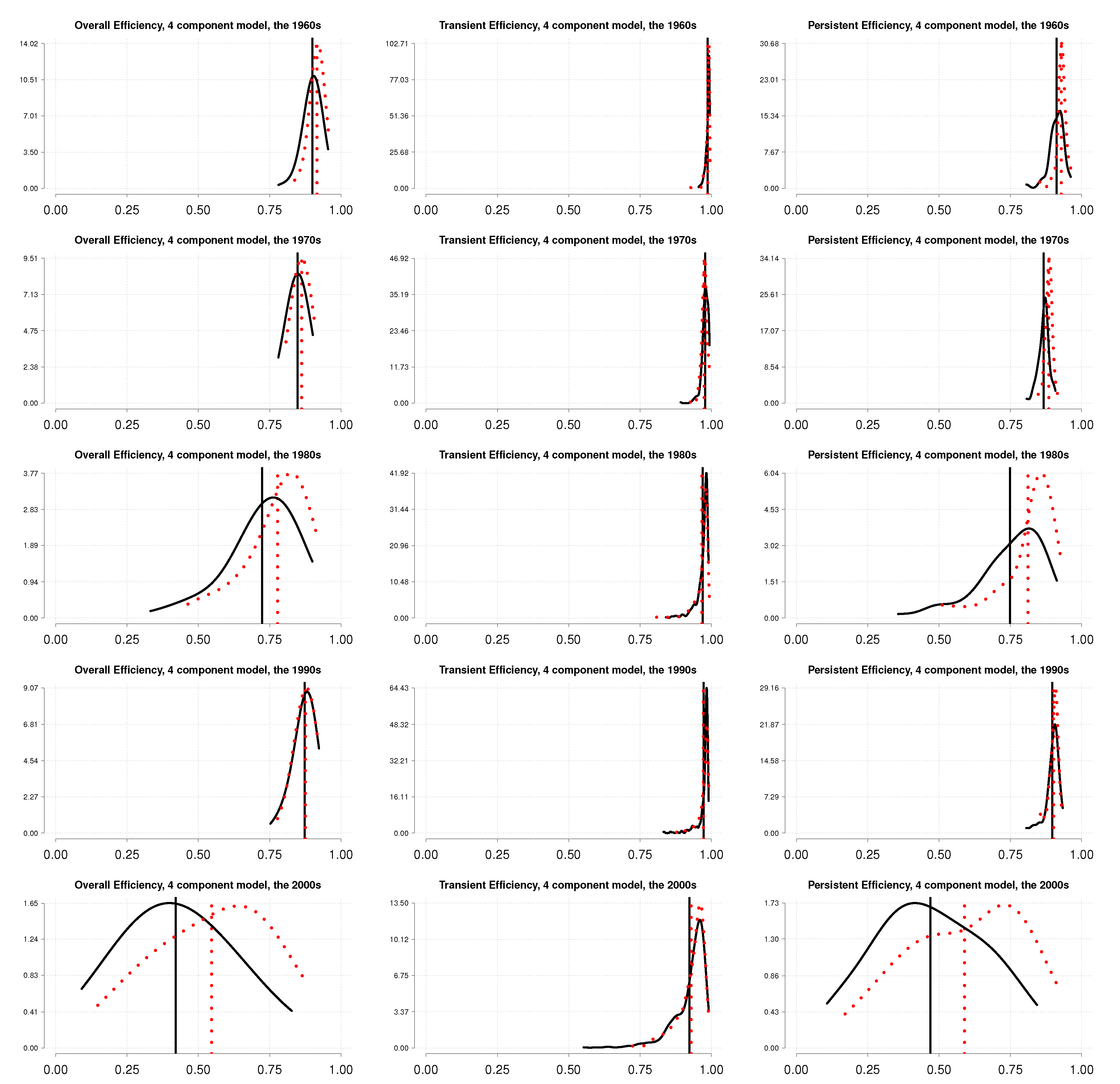
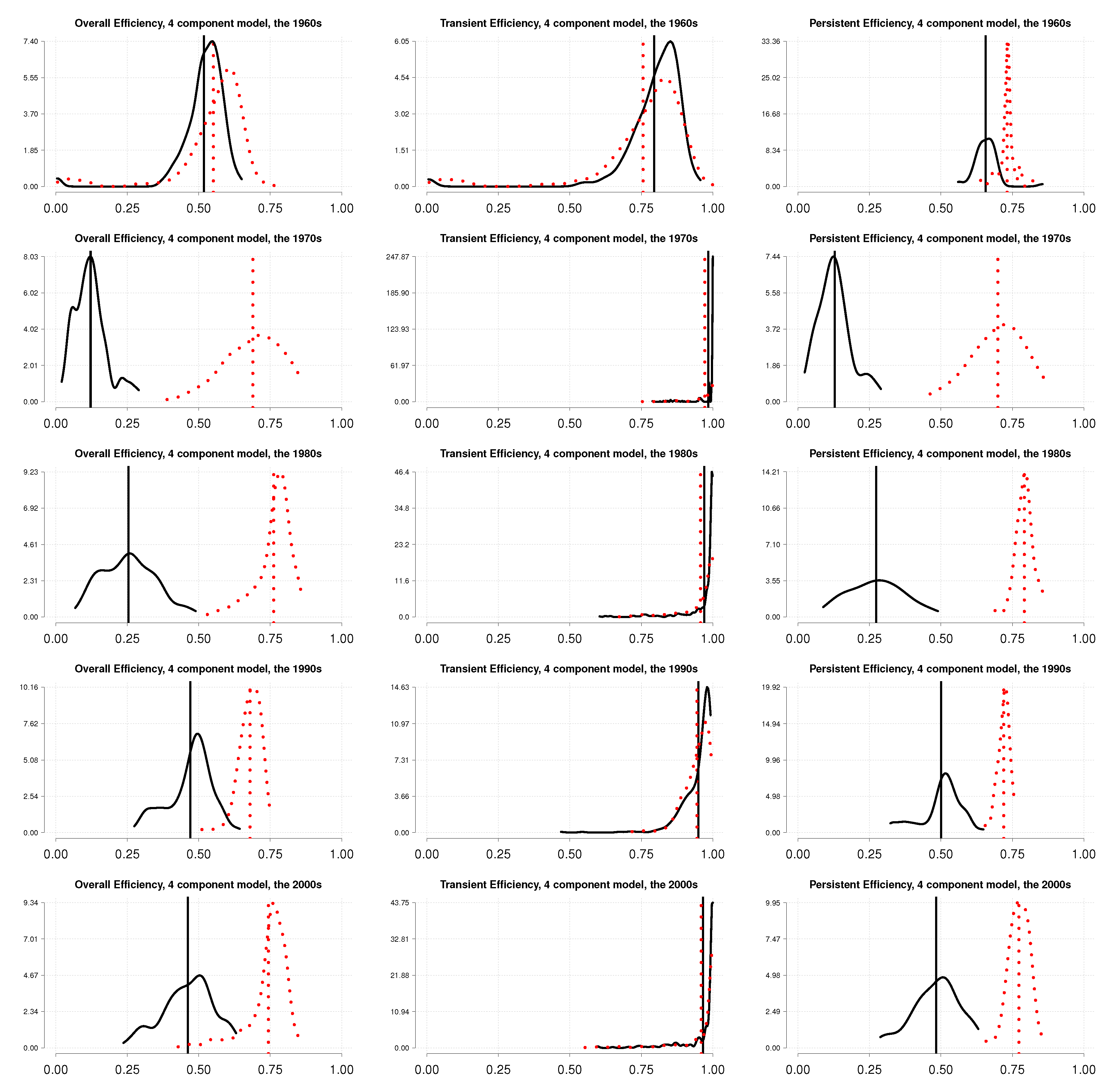
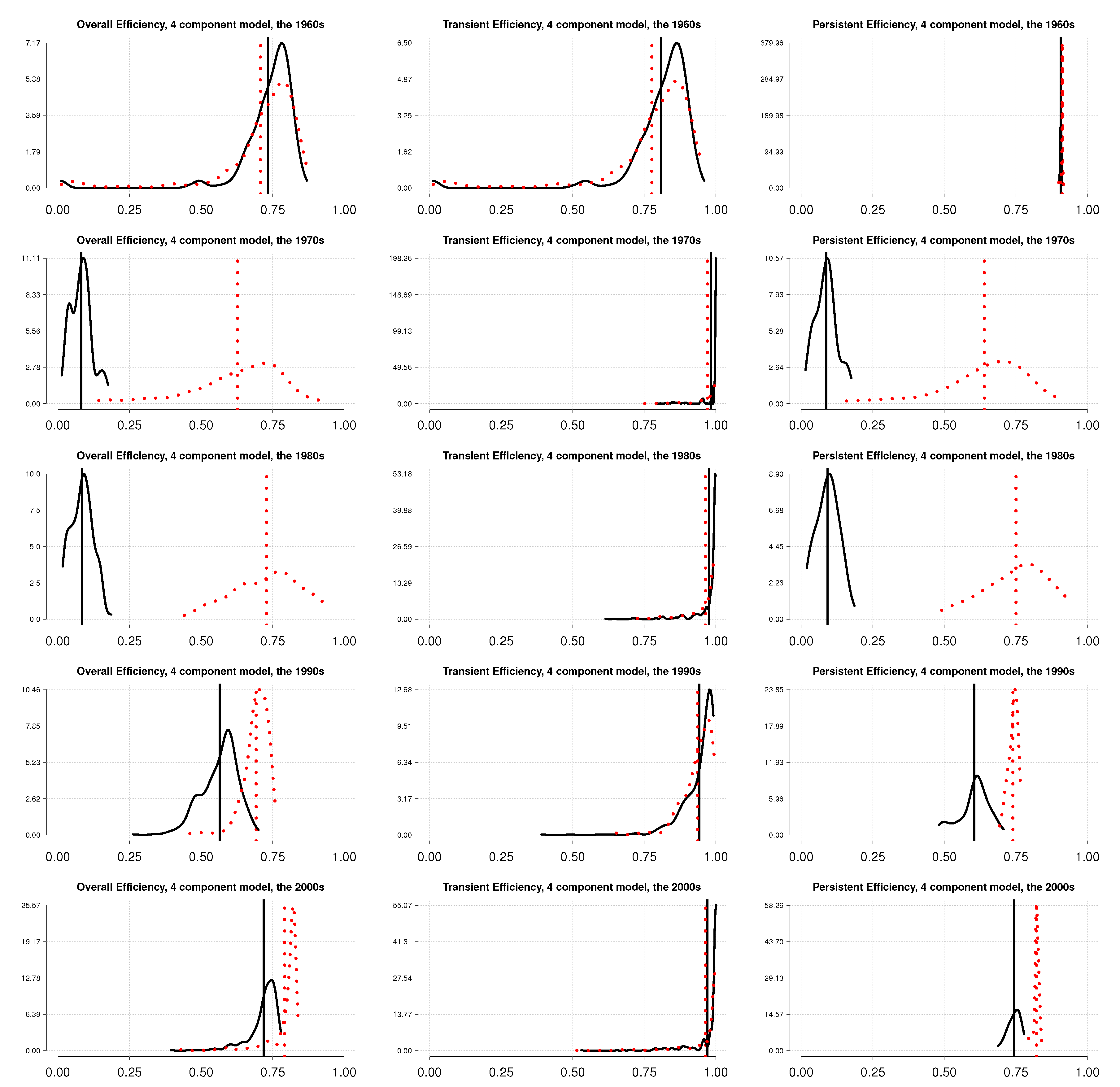
Figure 3 shows the evolution of average efficiency over time by the type of efficiency. Figure 4, Figure 5 and Figure 6 show densities of three types of efficiencies using the formula in (13) for models 1, 2, and 3, respectively by decade. The three columns in each of the there figures present overall, transient, and persistent efficiencies. Recall that the overall efficiency is the product of transient and persistent efficiencies. The rows from 1 to 5 show the decades from the 1960s through the 2000s.
Models 2 and 3 measure energy use efficiency directly. Since we are applying the 4-component model, the overall energy use efficiency is decomposed into the persistent and transient components. The left column of Figure 5 reveals that the overall energy use efficiency has deteriorated over time. This is also confirmed by the middle and lower panels in Figure 3. We note again that the efficiencies are not comparable as they are measured relative to decade-specific frontiers, however, we can gauge how industries performed within decades. The energy use efficiency was very low in the 1970s, which could be the result of the oil crisis, which hit all industries of the economy. The overall efficiency figure in the 1970s, however, additionally reveals that the high energy-intensive industries were hit much harder. We have seen in Table 1 that some industries consume energy up to about a third of their actual sales. The lower panels in the left column of Figure 5 and middle panel in Figure 3 indicate that high energy-intensive industries were rebounding from the oil crisis and were only short of reaching the level of overall energy use efficiency only in the 2000s. The levels of overall energy use efficiency are still very low by any standard for energy-intensive industries. The energy use efficiency of the low energy-intensive industries is quite stable relative to the decade specific frontiers. Clearly, if the share of energy costs in production is very low as Table 1 suggests, the shocks to energy use are not that profound.
Looking at the components of the overall efficiency, we again observe that the overall inefficiency is mainly rooted in the structural energy use inefficiency. The density of the transient efficiency with an exception of the 1960s is concentrated around unity. The structural efficiency is shown in the third column of Figure 5 and as persistent efficiency in Figure 3. For low energy-intensive industries, it remains virtually unchanged, albeit relative to the decade-specific frontier. As is expected after discussion of the overall efficiency, the persistent efficiency of the high energy-intensive industries plummeted in the 1970s and increased gradually only in the 2000s.

5.3. Discussion

It is worth noting that because we have estimated decade-specific frontiers, the efficiencies across decades are not directly comparable. Thus, we discuss the differences in efficiencies that are estimated relative to their frontiers. Overall, the level of efficiency is close to that reported by [44]. Based on Model 1, one result the becomes evident is that the industries move further away from the frontier over time. We cannot say whether this is because they were lagging behind technological progress or whether they were becoming less efficient. The second feature is that transient inefficiency is almost non-existent and input inefficiency almost completely stems from structural inefficiency. Third, we see a drop in efficiency in the 2000s, which can be attributed to downturns at the beginning of the 2000s as well as the financial crisis at the end of the decade. Finally, in terms of overall input inefficiency, both high and low energy-intensive industries perform similarly. Only in the 2000s, low energy-intensive industries seem to slightly over-perform high energy-intensive industries. We find confirmation for average levels in Figure 3.
Figure 6 summarizes the energy use efficiency for the third model, which is only slightly different from Model 2. The change that we observe in Figure 6 relative to Figure 5 is only quantitative. Conclusions that we drew from Figure 5 can be repeated for Model 3, so that the results of the third model can be seen as a robustness check.
It is difficult to say why we observe the so-called “energy paradox”. The US is known to promote energy efficiency policy (see, e.g., [33]). However, such policies lead to different outcomes. In Sweden for example, the adoption rate of energy efficiency measures is over 40% ([45]). Although financial intensive may be an important one in some industries and countries ([46]), Refernece [4] document lack of adoption, which constitutes the above paradox. The authors of [47] find that the most important barriers to more energy-efficient organization are internal economic and behavioral barriers. The authors of [48] name additional barriers including lack of interest in energy efficient technologies. Further, their findings suggest that adopting sound energy management practices is the most important driver of increased energy efficiency. Adopting cost-effective technologies is also important, but less so than the above-mentioned practices.

6. Conclusions

Energy is one of the most important inputs in manufacturing industries. It is a scarce input that is expensive in both monetary and environmental terms. Hence, both policymakers and businesses should consider the efficient use of this input in the long-term.
This study uses the stochastic frontier approach to measure energy use efficiency in the US manufacturing during the time period 1958–2011 using the NBER-CES Manufacturing Industry Database. When panel data are available as in our case, we advocate using the latest or the 4-component SF model. We concentrate on the most and least energy-intensive manufacturing industries. More specifically, we first define energy intensity as the costs of energy in total economic activity. Then for each of five decades, we identify the top 10% and bottom 10% energy-intensive industries. We apply the 4-component stochastic frontier model that decomposes overall efficiency into the long-term or persistent and short-term efficiencies. Our main findings suggest that energy use efficiency in US manufacturing hit hard by the oil shock in the 1970s and it did not rebound until the 2000s. The major culprit of the low overall energy use efficiency was structural inefficiency, a finding that goes hand in hand with the “energy paradox” (see, e.g., [4]). It seems that one of the ways to mitigate low levels of energy use efficiency should be to do more research along the lines of [5,47,48] to promote, adopt, and establish energy-efficient technologies as the new benchmark.

Author Contributions

Conceptualization, O.B. and S.C.K.; Methodology, O.B. and S.C.K.; Data collection S.C.K., formal analysis, O.B.; Writing—original draft preparation, O.B., Writing—Review and Editing, O.B. and S.C.K. All authors have read and agreed to the published version of the manuscript.

Funding

This research received no external funding.

Conflicts of Interest

All authors declare that they have no conflict of interest.

Appendix A

Table A1. Descriptive statistics by decade and by the intensity of energy use.
Time PeriodIndustriesMedianMeanSDMinMax
Y
The 1960sLeast energy-intensive832.951509.602214.5227.1017,931.30
The 1960sMost energy-intensive546.851251.662780.7979.7021,983.20
The 1970sLeast energy-intensive1438.453796.497199.52150.3043,128.30
The 1970sMost energy-intensive1128.703024.256117.26111.6054,446.30
The 1980sLeast energy-intensive3639.008997.8414,000.49286.8073,925.10
The 1980sMost energy-intensive2222.154855.718216.35136.6056,738.40
The 1990sLeast energy-intensive6168.6016,492.6723,594.40219.30145,256.20
The 1990sMost energy-intensive3312.506678.9310,571.67116.3056,895.00
The 2000sLeast energy-intensive7992.9019,773.5130,016.89149.1016,2181.80
The 2000sMost energy-intensive4243.009790.0617,328.47130.80123,129.80
K
The 1960sLeast energy-intensive400.851131.831841.056.209507.70
The 1960sMost energy-intensive1548.304670.4512,180.26111.1090,867.10
The 1970sLeast energy-intensive631.452049.623965.9527.6020,595.00
The 1970sMost energy-intensive2646.906482.3114,042.12257.7092,312.80
The 1980sLeast energy-intensive960.603075.505135.9752.8025,549.50
The 1980sMost energy-intensive2475.656780.6313,499.10236.7091,786.60
The 1990sLeast energy-intensive1338.904242.536078.2339.4027,170.30
The 1990sMost energy-intensive2933.306867.7712,257.56172.2070,528.90
The 2000sLeast energy-intensive1605.605526.128706.7357.3053,612.40
The 2000sMost energy-intensive3162.857044.3511,075.66165.7058,371.10
L
The 1960sLeast energy-intensive72.40127.50147.791.351018.47
The 1960sMost energy-intensive31.6683.17164.733.751145.57
The 1970sLeast energy-intensive76.74121.04122.079.94727.97
The 1970sMost energy-intensive30.7080.51150.273.901070.72
The 1980sLeast energy-intensive69.93116.73125.136.91686.44
The 1980sMost energy-intensive28.3859.7292.652.98762.71
The 1990sLeast energy-intensive64.72113.52117.394.49659.60
The 1990sMost energy-intensive26.6655.9274.332.09423.21
The 2000sLeast energy-intensive55.1892.3596.652.29487.05
The 2000sMost energy-intensive20.6339.7353.022.48380.14
NEM
The 1960sLeast energy-intensive432.60917.371687.3816.9015,436.70
The 1960sMost energy-intensive193.25555.571414.466.5011,553.60
The 1970sLeast energy-intensive787.602501.265759.8565.8037,855.40
The 1970sMost energy-intensive485.101460.073318.9614.7029,737.30
The 1980sLeast energy-intensive1832.105568.4110,423.51129.6050,316.50
The 1980sMost energy-intensive873.202306.364384.7727.7031,836.00
The 1990sLeast energy-intensive2950.909604.1416,286.3280.50102,924.30
The 1990sMost energy-intensive1276.853034.875404.5125.3029,446.20
The 2000sLeast energy-intensive3954.4010,175.9418,271.4463.80110,074.70
The 2000sMost energy-intensive1602.304847.6710,339.0624.8075,089.60
E
The 1960sLeast energy-intensive2.504.838.950.1075.70
The 1960sMost energy-intensive29.0070.23135.822.601056.00
The 1970sLeast energy-intensive7.0018.2235.640.40225.20
The 1970sMost energy-intensive96.30248.52513.127.105325.20
The 1980sLeast energy-intensive23.7056.5684.231.50348.40
The 1980sMost energy-intensive202.60494.83782.7420.305858.60
The 1990sLeast energy-intensive29.3066.0086.921.00350.40
The 1990sMost energy-intensive219.90486.65689.628.903570.80
The 2000sLeast energy-intensive35.0078.93126.080.70858.00
The 2000sMost energy-intensive355.60777.171158.6012.006775.10

Appendix B

Here we describe how to estimate the model in (11). To facilitate the discussion, rewrite
log q i t = r ( X i t , t r e n d ; ω ) + v 0 i u 0 i + v i t u i t
as
log q i t = r ( X i t , t r e n d ; ω ) + ϵ 0 i + ϵ i t ,
where ϵ i t = v i t u i t and ϵ 0 i = v 0 i u 0 i decompose the error term into two ‘composed error’ terms (both of which contain a two-sided and a one-sided error terms). Assume the most general case where all four components are heteroskedastic
σ u i t 2 = exp z u i t ψ u , i = 1 , , n , t = 1 , , T i ,
σ u 0 i 2 = exp z u 0 i ψ u 0 , i = 1 , , n ,
σ v i t 2 = exp z v i t ψ v , i = 1 , , n , t = 1 , , T i ,
σ v 0 i 2 = exp z v 0 i ψ v 0 , i = 1 , , n ,
where z u i t are the determinants of transient inefficiency, z u 0 i are the determinants of persistent inefficiency, and z v i t and z v 0 i define the heteroskedasticity functions of the noise and random effects. The homoskedastic error component is easily derived from (A2–A5) by setting the vector of determinants to a constant. For example if v i t is homoskedastic, z v i t is a vector of ones of length i = 1 n T i . The conditional density of ϵ i = ( ϵ i 1 , , ϵ i T i ) is given by
f ϵ i | ϵ 0 i = t = 1 T i 2 σ i t ϕ ϵ i t σ i t Φ ϵ i t λ i t σ i t ,
where σ i t = exp z u i t ψ u + exp z v i t ψ v 1 / 2 and λ i t = exp z u i t ψ u / exp z v i t ψ v 1 / 2 .
Integrate ϵ 0 i (the distribution of which we know) out to get the unconditional density of ϵ i
f ϵ i = t = 1 T i 2 σ i t ϕ ϵ i t σ i t Φ ϵ i t λ i t σ i t × 2 σ 0 i ϕ ϵ 0 i σ 0 i Φ ϵ 0 i λ 0 i σ 0 i d ϵ 0 i ,
where σ 0 i = [ exp z u 0 i ψ u 0 + exp z v 0 i ψ v 0 ] 1 / 2 and λ 0 i = [ exp z u 0 i ψ u 0 / exp z v 0 i ψ v 0 ] 1 / 2 . The log-likelihood function for the i-th observation of model (A1) is therefore given by
log L i β , ψ u 0 , ψ v 0 , ψ u , ψ v = log + t = 1 T i 2 σ i t ϕ r i t ϵ 0 i σ i t × Φ ( r i t ϵ 0 i ) λ i t σ i t 2 σ 0 i ϕ ϵ 0 i σ 0 i Φ ϵ 0 i λ 0 i σ 0 i d ϵ 0 i = log + t = 1 T i 2 σ i t ϕ ϵ i t σ i t Φ ϵ i t λ i t σ i t × 2 σ 0 i ϕ ϵ 0 i σ 0 i Φ ϵ 0 i λ 0 i σ 0 i d ϵ 0 i ,
where ϵ i t = r i t ( v 0 i + u 0 i ) and r i t = log q i t r ( X i t , t r e n d ; ω ) . We rely on the Monte-Carlo integration as a method to approximate the integral in (A6). For estimation purposes, we write ϵ 0 i = [ exp z u 0 i ψ u 0 ] 1 / 2 V i + [ exp z v 0 i ψ v 0 ] 1 / 2 | U i | , where both V i and U i are standard normal random variables. The resulting simulated log-likelihood function for the i-th observation is
log L i S β , ψ u 0 , ψ v 0 , ψ u , ψ v = log 1 R r = 1 R t = 1 T i 2 σ i t ϕ r i t ( [ exp z u 0 i ψ u 0 ] 1 / 2 V i r + [ exp z v 0 i ψ v 0 ] 1 / 2 | U i r | ) σ i t × Φ [ r i t ( [ exp z u 0 i ψ u 0 ] 1 / 2 V i r + [ exp z v 0 i ψ v 0 ] 1 / 2 | U i r | ) ] λ σ i t = log 1 R r = 1 R t = 1 T i 2 σ ϕ ϵ i t r σ Φ ϵ i t r λ σ ,
where V i r and U i r are R random deviates from the standard normal distribution, and ϵ i t r = r i t ( [ exp z u 0 i ψ u 0 ] 1 / 2 V i r + [ exp z v 0 i ψ v 0 ] 1 / 2 | U i r | ) . R is the number of draws for approximating the log-likelihood function. The full log-likelihood is the sum of panel-i specific log-likelihoods given in (A7).
We use the results of [39] to calculate persistent and time-varying cost efficiencies. Using the moment generating function of the closed skew normal distribution, the conditional means of u 0 i , u i 1 , , u i T i are given by:
E ( exp { t u i } | r i ) = Φ ¯ T i + 1 R i r i + Λ i t , Λ i Φ ¯ T i + 1 R i r i , Λ i × exp t R i r i + 0.5 t Λ i t ,
where r i = r i 1 , , r i T i , A = [ 1 T i I T i ] , 1 T i is the column vector of length T i and I T i is the identity matrix of dimension T i , the diagonal elements of V i are exp z u 0 i ψ u 0 exp z u i t ψ u , Σ i = exp z v i t ψ v I T i + exp z v 0 i ψ v 0 1 T i 1 T i , Λ i = V i V i A Σ i + A V i A 1 A V i = V i 1 + A Σ i 1 A 1 , R i = V i A Σ i + A V i A 1 = Λ i A Σ i 1 , ϕ q x , μ , Ω is the density function of a q-dimensional normal variable with expected value μ and variance Ω and Φ ¯ q μ , Ω is the probability that a q-variate normal variable of expected value μ and variance Ω belongs to the positive orthant., u i = ( u 0 i , u i 1 , , u i T i ) , and t is a row of the identity matrix of dimension ( T i + 1 ) . If t is the τ -th row, Equation (A8) provides the conditional expected value of the τ -th component of the cost efficiency vector exp u i . In particular, for τ = 1 , we get the conditional expected value of the persistent technical efficiency.

References

  1. Menghi, R.; Papetti, A.; Germani, M.; Marconi, M. Energy efficiency of manufacturing systems: A review of energy assessment methods and tools. J. Clean. Prod. 2019, 240, 118276. [Google Scholar] [CrossRef]
  2. Kanellakis, M.; Martinopoulos, G.; Zachariadis, T. European energy policy-A review. Energy Policy 2013, 62, 1020–1030. [Google Scholar] [CrossRef]
  3. Wang, C.N.; Ho, H.X.T.; Hsueh, M.H. An integrated approach for estimating the energy efficiency of seventeen countries. Energies 2017, 10, 1597. [Google Scholar] [CrossRef]
  4. Gerarden, T.D.; Newell, R.G.; Stavins, R.N. Assessing the Energy-Efficiency Gap. J. Econ. Lit. 2017, 55, 1486–1525. [Google Scholar] [CrossRef] [Green Version]
  5. Blass, V.; Corbett, C.J.; Delmas, M.A.; Muthulingam, S. Top management and the adoption of energy efficiency practices: Evidence from small and medium-sized manufacturing firms in the US. Energy 2014, 65, 560–571. [Google Scholar] [CrossRef] [Green Version]
  6. Boyd, G.A.; Lee, J.M. Measuring plant level energy efficiency and technical change in the U.S. metal-based durable manufacturing sector using stochastic frontier analysis. Energy Econ. 2019, 81, 159–174. [Google Scholar] [CrossRef] [Green Version]
  7. Filipović, S.; Verbič, M.; Radovanović, M. Determinants of energy intensity in the European Union: A panel data analysis. Energy 2015, 92, 547–555. [Google Scholar] [CrossRef]
  8. Bentzen, J. Estimating the rebound effect in US manufacturing energy consumption. Energy Econ. 2004, 26, 123–134. [Google Scholar] [CrossRef]
  9. Bartelsman, E.J.; Gray, W. The NBER Manufacturing Productivity Database; Working Paper 205; National Bureau of Economic Research: Cambridge, MA, USA, 1996. [Google Scholar] [CrossRef] [Green Version]
  10. Parker, S.; Liddle, B. Energy efficiency in the manufacturing sector of the OECD: Analysis of price elasticities. Energy Econ. 2016, 58, 38–45. [Google Scholar] [CrossRef]
  11. Badunenko, O.; Kumbhakar, S.C. Economies of scale, technical change and persistent and time-varying cost efficiency in Indian banking: Do ownership, regulation and heterogeneity matter? Eur. J. Oper. Res. 2017, 260, 789–803. [Google Scholar] [CrossRef] [Green Version]
  12. Wei, T. Impact of energy efficiency gains on output and energy use with Cobb-Douglas production function. Energy Policy 2007, 35, 2023–2030. [Google Scholar] [CrossRef]
  13. Saunders, H.D. Historical evidence for energy efficiency rebound in 30 US sectors and a toolkit for rebound analysts. Technol. Forecast. Soc. Chang. 2013, 80, 1317–1330. [Google Scholar] [CrossRef]
  14. Allcott, H.; Knittel, C.; Taubinsky, D. Tagging and Targeting of Energy Efficiency Subsidies. Am. Econ. Rev. 2015, 105, 187–191. [Google Scholar] [CrossRef] [Green Version]
  15. Kumbhakar, S.C.; Lovell, C.A.K. Stochastic Frontier Analysis; Cambridge University Press: Cambridge, UK, 2000. [Google Scholar] [CrossRef]
  16. Färe, R.; Grosskopf, S.; Lovell, C.A.K. Production Frontiers; Cambridge University Press: Cambridge, UK, 1994. [Google Scholar] [CrossRef]
  17. Kumbhakar, S.C. The Measurement and Decomposition of Cost-Inefficiency: The Translog Cost System. Oxf. Econ. Pap. New Ser. 1991, 43, 667–683. [Google Scholar] [CrossRef]
  18. Kumbhakar, S.C.; Heshmati, A. Efficiency Measurement in Swedish Dariy Farms: An Application of Rotating Panel Data. Am. J. Agric. Econ. 1995, 77, 660–674. [Google Scholar] [CrossRef]
  19. Kumbhakar, S.C.; Hjalmarsson, L. Technical Efficiency and Technical Progress in Swedish Dairy Farms. In The Measurement of Productive Efficiency. Techniques and Applications; Fried, H.O., Lovell, C.A.K., Schmidt, S.S., Eds.; Oxford University Press: Oxford, UK, 1993; pp. 256–270. [Google Scholar]
  20. Kumbhakar, S.C.; Hjalmarsson, L. Labour-Use Efficiency in Swedish Social Insurance Offices. J. Appl. Econ. 1995, 10, 33–47. [Google Scholar] [CrossRef]
  21. Greene, H.W. Reconsidering Heterogeneity in Panel Data Estimators of the Stochastic Frontier Model. J. Econ. 2005, 126, 269–303. [Google Scholar] [CrossRef]
  22. Kumbhakar, S.C.; Lien, G.; Hardaker, J.B. Technical Efficiency in Competing Panel Data Models: A Study of Norwegian Grain Farming. J. Product. Anal. 2014, 41, 321–337. [Google Scholar] [CrossRef]
  23. Mukherjee, K. Energy use efficiency in U.S. manufacturing: A nonparametric analysis. Energy Econ. 2008, 30, 76–96. [Google Scholar] [CrossRef]
  24. Mukherjee, K. Energy use efficiency in the Indian manufacturing sector: An interstate analysis. Energy Policy 2008, 36, 662–672. [Google Scholar] [CrossRef]
  25. Zhou, P.; Ang, B.W. Linear programming models for measuring economy-wide energy efficiency performance. Energy Policy 2008, 36, 2911–2916. [Google Scholar] [CrossRef]
  26. Mousavi-Avval, S.H.; Rafiee, S.; Jafari, A.; Mohammadi, A. Improving energy use efficiency of canola production using data envelopment analysis (DEA) approach. Energy 2011, 36, 2765–2772. [Google Scholar] [CrossRef]
  27. Sueyoshi, T.; Yuan, Y.; Goto, M. A literature study for DEA applied to energy and environment. Energy Econ. 2017, 62, 104–124. [Google Scholar] [CrossRef]
  28. Boyd, G.A. A Method for Measuring the Efficiency Gap between Average and Best Practice Energy Use: The ENERGY STAR Industrial Energy Performance Indicator. J. Ind. Ecol. 2005, 9, 51–65. [Google Scholar] [CrossRef] [Green Version]
  29. Boyd, G.A. Estimating Plant Level Energy Efficiency with a Stochastic Frontier. Energy J. 2008, 29, 23–43. [Google Scholar] [CrossRef]
  30. Filippini, M.; Hunt, L.C. US residential energy demand and energy efficiency: A stochastic demand frontier approach. Energy Econ. 2012, 34, 1484–1491. [Google Scholar] [CrossRef] [Green Version]
  31. Shui, H.; Jin, X.; Ni, J. Manufacturing productivity and energy efficiency: A stochastic efficiency frontier analysis. Int. J. Energy Res. 2015, 39, 1649–1663. [Google Scholar] [CrossRef] [Green Version]
  32. Farsi, M.; Filippini, M.; Greene, W. Application of Panel Data Models in Benchmarking Analysis of the Electricity Distribution Sector. Ann. Public Coop. Econ. 2006, 77, 271–290. [Google Scholar] [CrossRef] [Green Version]
  33. Filippini, M.; Hunt, L.C. Measuring persistent and transient energy efficiency in the US. Energy Effic. 2016, 9, 663–675. [Google Scholar] [CrossRef] [Green Version]
  34. Kumbhakar, S.C.; Lien, G. Yardstick Regulation of Electricity Distribution – Disentangling Short-run and Long-run Inefficiencies. Energy J. 2017, 38, 1944–9089. [Google Scholar] [CrossRef]
  35. Kumbhakar, S.C. Specification and estimation of multiple output technologies: A primal approach. Eur. J. Oper. Res. 2013, 231, 465–473. [Google Scholar] [CrossRef]
  36. Diewert, W.E. Functional Forms for Revenue and Factor Requirements Functions. Int. Econ. Rev. 1974, 15, 119–130. [Google Scholar] [CrossRef]
  37. Aigner, D.; Lovell, C.A.K.; Schmidt, P. Formulation and estimation of stochastic frontier production function models. J. Econ. 1977, 6, 21–37. [Google Scholar] [CrossRef]
  38. Meeusen, W.; van den Broeck, J. Efficiency estimation from {C}obb-{D}ouglas production functions with composed error. Int. Econ. Rev. 1977, 18, 435–444. [Google Scholar] [CrossRef]
  39. Colombi, R.; Kumbhakar, S.C.; Martini, G.; Vittadini, G. Closed-skew normality in stochastic frontiers with individual effects and long/short-run efficiency. J. Product. Anal. 2014, 42, 123–136. [Google Scholar] [CrossRef]
  40. Tsionas, E.G.; Kumbhakar, S.C. Firm Heterogeneity, Persistent And Transient Technical Inefficiency: A Generalized True Random Effects model. J. Appl. Econ. 2014, 29, 110–132. [Google Scholar] [CrossRef]
  41. Battese, G.E.; Coelli, T.J. Frontier production functions, technical efficiency and panel data: With application to paddy farmers in India. J. Product. Anal. 1992, 3, 153–169. [Google Scholar] [CrossRef]
  42. Cornwell, C.; Schmidt, P.; Sickles, R.C. Production frontiers with cross-sectional and time-series variation in efficiencylevels. J. Econ. 1990, 46, 185–200. [Google Scholar] [CrossRef]
  43. Kumbhakar, S.C. Production frontiers, panel data, and time-varying technical inefficiency. J. Econ. 1990, 46, 201–211. [Google Scholar] [CrossRef]
  44. Hsiao, W.L.; Hu, J.L.; Hsiao, C.; Chang, M.C. Energy Efficiency of the Baltic Sea Countries: An Application of Stochastic Frontier Analysis. Energies 2019, 12, 104. [Google Scholar] [CrossRef] [Green Version]
  45. Thollander, P.; Danestig, M.; Rohdin, P. Energy policies for increased industrial energy efficiency: Evaluation of a local energy programme for manufacturing SMEs. Energy Policy 2007, 35, 5774–5783. [Google Scholar] [CrossRef] [Green Version]
  46. Thollander, P.; Backlund, S.; Trianni, A.; Cagno, E. Beyond barriers—A case study on driving forces for improved energy efficiency in the foundry industries in Finland, France, Germany, Italy, Poland, Spain, and Sweden. Appl. Energy 2013, 111, 636–643. [Google Scholar] [CrossRef] [Green Version]
  47. Brunke, J.C.; Johansson, M.; Thollander, P. Empirical investigation of barriers and drivers to the adoption of energy conservation measures, energy management practices and energy services in the Swedish iron and steel industry. J. Clean. Prod. 2014, 84, 509–525. [Google Scholar] [CrossRef] [Green Version]
  48. Trianni, A.; Cagno, E.; Worrell, E.; Pugliese, G. Empirical investigation of energy efficiency barriers in Italian manufacturing SMEs. Energy 2013, 49, 444–458. [Google Scholar] [CrossRef]
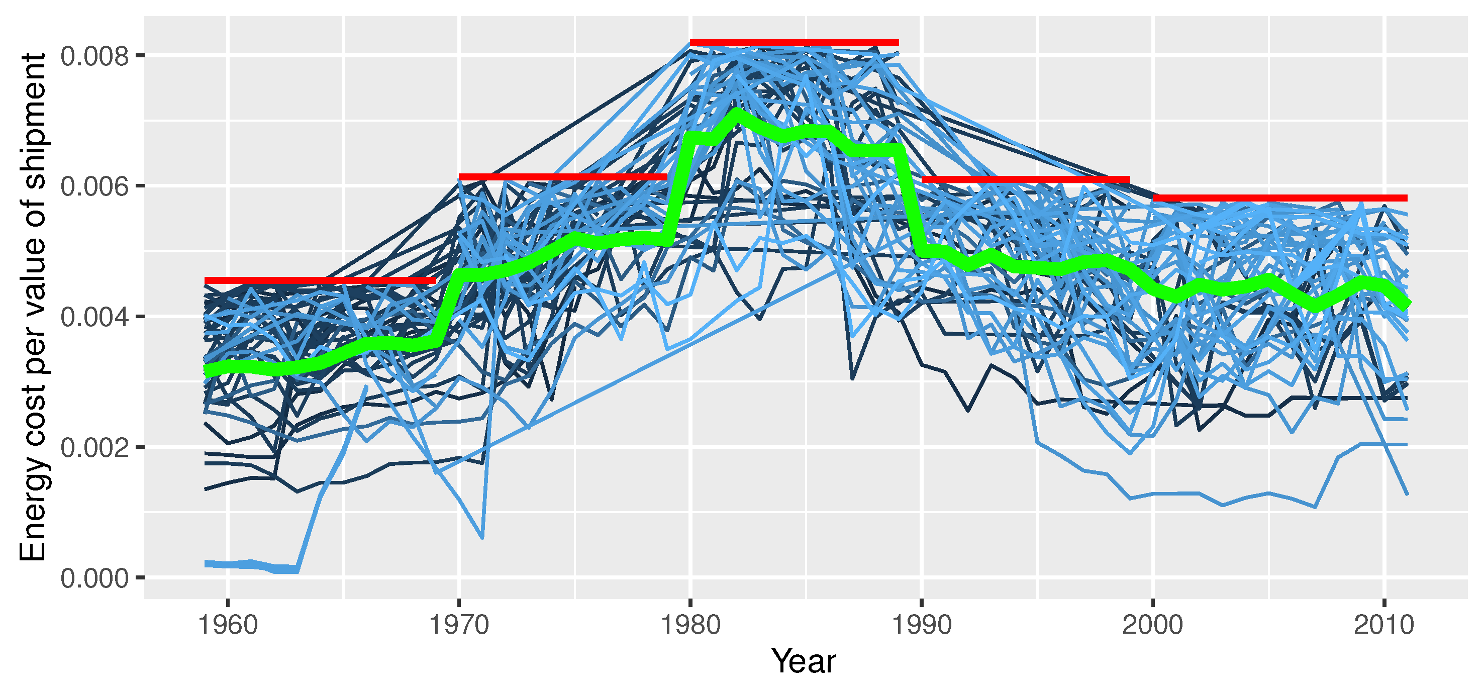
Figure 1. Energy intensity of industries. Shown are industries whose energy intensity are lower than the 10th percentile in a respective decade. Notes: Horizontal red lines show the 10th percentile of energy intensity in a respective decade. The bold green solid line shows the mean of energy intensity for industries whose energy intensity are lower than the 10th percentile in a respective decade.
Energies 13 03954 g001
Figure 2. Energy intensity of industries. Shown are industries whose energy intensity exceeds the 90th percentile in a respective decade. Notes: Horizontal red lines show the 90th percentile of energy intensity in a respective decade. The bold green solid line shows the mean of energy intensity for industries whose energy intensity exceeds the 90th percentile in a respective decade.
Energies 13 03954 g002
Figure 3. Average efficiency by year, energy intensity, and type of efficiency. The abbreviation HI stands for high intensity and LI means low intensity. Notes: The dotted time-series lines are for the high and solid lines are for low intensity industries.
Energies 13 03954 g003
Figure 4. Overall, transient and persistent energy efficiency, Model 1. Notes: Solid black curves are high energy-intensive industries, dotted red curves are low energy-intensive industries. Vertical lines are respective mean values.
Energies 13 03954 g004
Figure 5. Overall, transient and persistent energy efficiency, Model 2. Notes: Solid black curves are high energy-intensive industries, dotted red curves are low energy-intensive industries. Vertical lines are respective mean values.
Energies 13 03954 g005
Figure 6. Overall, transient and persistent energy efficiency, Model 3. Notes: Solid black curves are high energy-intensive industries, dotted red curves are low energy-intensive industries. Vertical lines are respective mean values.
Energies 13 03954 g006
Table 1. Descriptive statistics of energy intensity by decade and by the intensity of energy use.
Time PeriodIndustriesMedianMeanSDMinMax
AllBoth most and least energy-intensive0.04170.04890.05650.000080.3414
AllLeast energy-intensive0.00450.00460.00150.000080.0082
AllMost energy-intensive0.06900.08730.05270.031690.3414
The 1960sLeast energy-intensive0.00350.00330.00110.000080.0046
The 1960sMost energy-intensive0.04890.06270.03330.031690.2006
The 1970sLeast energy-intensive0.00490.00480.00090.000610.0061
The 1970sMost energy-intensive0.07060.08810.05130.042580.3311
The 1980sLeast energy-intensive0.00680.00650.00120.003040.0082
The 1980sMost energy-intensive0.08500.11280.06390.054260.3414
The 1990sLeast energy-intensive0.00470.00460.00100.001210.0061
The 1990sMost energy-intensive0.06450.08190.04770.042020.2775
The 2000sLeast energy-intensive0.00420.00420.00110.001080.0058
The 2000sMost energy-intensive0.07110.09210.05130.046300.2709
Table 2. Model 1 as in Equation (3). Dependent variable is log E . z-values in parentheses.
ParameterThe 1960sThe 1970sThe 1980sThe 1990sThe 2000s
Intercept1.430(24.95)1.094(6.44)1.635(7.17)1.109(6.55)2.459(16.77)
0.5 * log(K/E) 2 0.020(1.51)0.019(0.39)0.028(0.24)0.091(3.14)−0.031(−1.37)
0.5 * log(L/E) 2 0.107(9.48)−0.041(−3.25)0.092(4.83)−0.031(−1.77)0.072(2.69)
0.5 * log(NEM/E) 2 0.189(17.96)0.124(6.50)0.187(6.92)0.160(6.52)0.071(2.56)
0.5 * log(Y) 2 0.002(0.41)−0.017(−0.95)0.044(14.23)0.043(21.12)0.054(29.65)
0.5 * Trend 2 0.003(4.33) 5.8 × 10 4 (−0.45)0.004(3.40)0.003(2.72)0.003(4.58)
log(K/E)−0.082(−2.68)0.118(0.92)−0.142(−1.21)0.026(0.32)0.023(0.32)
log(K/E) * log(L/E)0.039(4.53)0.061(6.54)0.002(0.08)−0.031(−2.72)−0.052(−2.78)
log(K/E) * log(NEM/E)−0.037(−3.89)−0.057(−2.24)−0.006(−0.10)−0.064(−2.88)0.058(2.45)
log(K/E) * log(Y)0.020(3.53)0.002(0.29)0.042(2.29)0.016(3.78)0.023(2.52)
log(K/E) * Trend0.005(2.83)0.006(1.12)0.005(1.59)0.004(1.93)0.002(1.32)
log(L/E)0.493(17.03)0.418(4.42)0.501(6.96)0.862(11.33)0.903(10.50)
log(L/E) * log(NEM/E)−0.148(−10.56)−0.032(−2.54)−0.137(−4.89)−0.016(−1.08)−0.059(−2.67)
log(L/E) * log(Y)−0.011(−1.26)−0.030(−1.42)0.024(1.63)−0.051(−6.52)−0.032(−7.93)
log(L/E) * Trend0.006(5.75)−0.002(−0.42)−0.001(−0.84)0.002(0.98)−0.006(−2.65)
log(NEM/E)0.431(23.41)0.242(8.68)0.363(4.87)0.331(5.19)0.061(1.06)
log(NEM/E) * log(Y)−0.018(−2.14)0.018(1.00)−0.063(−3.79)−0.028(−6.73)−0.023(−2.72)
log(NEM/E) * Trend−0.007(−6.50)−0.005(−1.01)−0.005(−2.51)−0.007(−3.93)0.003(1.62)
log(Y)−0.932(−76.70)−0.772(−10.27)−1.014(−37.43)−0.991(−65.69)−1.059(−60.64)
log(Y) * Trend 1.1 × 10 4 (−0.16)−0.001(−0.70)−0.001(−0.50)−0.001(−1.49)−0.005(−4.01)
Trend−0.017(−2.39)0.017(1.14)0.006(0.28)0.020(2.40)0.012(0.81)
Random effects component: log σ v 0 i 2
lnVARv0iIntercept−3.820(−95.00)−2.548(−15.71)−2.978(−12.85)−2.066(−65.46)−3.204(−67.88)
Persistent inefficiency component: log σ u 0 i 2
lnVARu0iIntercept−4.570(−56.15)−3.936(−5.12)−2.197(−21.74)−3.943(−44.12)-0.764(−23.66)
Random noise component: log σ v i t 2
lnVARvitIntercept−6.571(−97.67)−6.445(−49.51)−6.455(−47.84)−6.379(−44.86)−7.431(−44.92)
Transient inefficiency component: log σ u i t 2
lnVARuitIntercept−4.548(−4.04)−7.251(−4.62)−3.859(−8.03)−5.909(−3.74)−3.658(−13.88)
lnVARuitTrend−1.372(−3.10)0.462(0.80)−1.469(−5.51)−0.931(−2.12)−0.634(−6.76)
lnVARuitTrend 2 0.098(2.91)−0.067(−1.17)0.139(5.54)0.104(3.09)0.056(7.84)
Sample Size
N10511310498109
i = 1 N T i 9688508358171005
Sim. logL1497.731144.891055.051021.781067.50
Table 3. Model 2 as in Equation (8). Dependent variable is log E . z-values in parentheses.
ParameterThe 1960sThe 1970sThe 1980sThe 1990sThe 2000s
Intercept−8.488(−21.97)−4.999(−8.78)−4.001(−42.61)−7.573(−33.18)−7.973(−26.42)
0.5 * log(K) 2 0.019(0.70)0.131(1.90)0.057(2.29)−0.038(−1.79)−0.130(−5.22)
0.5 * log(L) 2 −0.782(−15.67)−0.087(−3.52)0.106(6.43)0.047(1.26)−0.049(−1.44)
0.5 * log(NEM) 2 −0.486(−5.73)0.258(6.97)0.127(4.43)0.791(10.17)−0.256(−15.50)
0.5 * log(Y) 2 0.849(6.90)0.353(7.99)−0.310(−6.63)0.300(5.12)−0.678(−24.19)
0.5 * Trend 2 7.2 × 10 4 (−0.30)−0.009(−3.52)−0.027(−15.93)−0.006(−3.63)−0.017(−11.00)
log(K)1.504(26.62)−0.552(−2.51)−0.270(−3.07)−0.014(−0.20)0.129(1.03)
log(K) * log(L)0.349(9.52)−0.038(−0.97)−0.130(−4.60)−0.055(−1.17)−0.007(−0.16)
log(K) * log(NEM)−0.344(−10.11)0.198(2.41)−0.149(−10.31)0.068(1.75)−0.124(−3.52)
log(K) * log(Y)−0.158(−9.43)−0.150(−4.94)0.257(21.41)0.056(2.08)0.275(16.63)
log(K) * Trend0.023(7.19)0.008(1.50)−0.020(−6.35)0.004(1.15)0.006(1.55)
log(L)1.022(11.95)−0.138(−1.37)0.464(7.54)0.448(4.34)−0.114(−2.11)
log(L) * log(NEM)0.982(9.05)−0.080(−1.22)0.007(0.19)−0.413(−4.51) 8.7 × 10 5 ( 3.2 × 10 3 )
log(L) * log(Y)−0.758(−7.77)0.167(1.90)0.017(0.36)0.400(4.23)0.065(1.25)
log(L) * Trend−0.023(−2.89)−0.006(−0.73)0.003(0.76)−0.007(−1.45) 2.1 × 10 4 (−0.04)
log(NEM)0.763(5.20)0.148(0.64)0.527(4.98)0.792(8.17)0.005(0.04)
log(NEM) * log(Y)−0.052(−1.69)−0.405(−8.70)0.007(1.01)−0.684(−66.10)0.339(29.12)
log(NEM) * Trend0.039(3.99)0.001(0.11)−0.019(−2.58)0.002(0.26)−0.005(−0.94)
log(Y)−0.432(−1.28)1.182(5.33)0.393(2.43)0.954(12.19)1.475(6.87)
log(Y) * Trend−0.030(−1.75)0.004(0.20)0.036(2.78)−0.002(−0.13)0.005(0.43)
Trend−0.044(−2.14)0.061(2.18)0.105(4.91)0.018(0.78)0.085(3.62)
Random effects component: log σ v 0 i 2
lnVARv0iIntercept0.567(25.03)−2.153(−24.98)−1.542(−37.01)−0.367(−5.24)−0.643(−26.28)
Persistent inefficiency component: log σ u 0 i 2
lnVARu0iIntercept−1.363(−23.33)0.459(10.69)−0.469(−15.46)−0.730(−9.23)−1.022(−19.82)
Random noise component: log σ v i t 2
lnVARvitIntercept−6.180(−25.73)−4.043(−66.60)−4.723(−63.28)−4.185(−57.02)−4.079(−74.23)
Transient inefficiency component: log σ u i t 2
lnVARuitIntercept−3.195(−14.71)−1.013(−1.92)−17.732(−5.89)−9.850(−8.06)−0.320(−0.88)
lnVARuitTrend0.214(7.36)−2.225(−4.11)1.531(5.13)0.673(5.07)−1.666(−8.42)
Sample Size
N10511310498109
i = 1 N T i 9688508358171005
Sim. logL−274.84155.72328.12163.25136.60
Table 4. Model 3 as in Equation (10). Dependent variable is log E . z-values in parentheses.
ParameterThe 1960sThe 1970sThe 1980sThe 1990sThe 2000s
Intercept−5.788(−27.29)−4.111(−13.84)−4.328(−19.92)−6.833(−27.68)−6.349(−19.86)
0.5 * log(K) 2 −0.055(−1.54)0.091(3.74)0.011(0.67)−0.046(−1.66)−0.109(−5.19)
0.5 * log(L) 2 −0.480(−13.99)−0.036(−1.30)0.246(19.91)0.183(8.27)0.186(7.85)
0.5 * log(NEM) 2 −0.203(−1.30)−0.010(−0.50)0.047(1.19)0.176(5.53)0.069(3.56)
0.5 * log(wE/wY) 2 −0.340(−7.45)−0.005(−0.24)−0.071(−1.55)−0.067(−0.23)−0.105(−2.50)
0.5 * Trend 2 3.5 × 10 4 (0.13)−0.011(−4.85)−0.021(−12.95)−0.007(−4.07)−0.018(−12.46)
log(K)1.180(8.92)−0.377(−3.85)0.275(5.94)0.852(18.24)1.061(14.19)
log(K) * log(L)0.207(6.18)0.020(0.64)0.029(1.27)0.060(1.30)0.065(2.07)
log(K) * log(NEM)−0.264(−108.79)−0.005(−0.72)−0.003(−1.84)−0.035(−12.27)−0.012(−3.90)
log(K) * log(wE/wY)0.088(0.93)−0.003(−0.10)0.113(3.90)−0.075(−0.87)−0.070(−1.43)
log(K) * Trend0.016(5.66)0.019(5.67)−0.006(−3.55)0.009(3.87)0.006(2.00)
log(L)−0.426(−1.15)0.675(8.24)0.095(1.04)1.736(26.02)0.452(5.57)
log(L) * log(NEM)0.336(3.92)−0.057(−1.93)−0.146(−4.47)−0.311(−6.62)−0.163(−4.85)
log(L) * log(wE/wY)0.050(0.47)0.151(3.91)−0.031(−0.71)0.034(0.28)0.055(1.06)
log(L) * Trend−0.027(−6.74)−0.010(−1.85)0.019(7.95)0.001(0.40)0.010(2.29)
log(NEM)1.128(2.28)0.706(11.62)0.636(4.38)0.292(3.91)0.561(14.16)
log(NEM) * log(wE/wY)−0.053(−0.39)−0.090(−2.58)−0.079(−1.62)−0.111(−1.01)−0.019(−0.49)
log(NEM) * Trend0.023(4.45)−0.004(−0.83)−0.006(−2.29)−0.013(−3.77)−0.006(−1.55)
log(wE/wY)−0.542(−2.10)0.114(0.76)−0.094(−0.54)1.371(2.97)0.533(1.91)
log(wE/wY) * Trend−0.005(−0.62)0.024(5.10)0.021(4.38)0.013(0.65)0.011(1.43)
Trend−0.093(−2.22)0.092(4.71)0.113(8.89)0.056(3.85)0.111(6.40)
Random effects component: log σ v 0 i 2
lnVARv0iIntercept0.769(20.77)−3.036(−20.12)−3.841(−37.08)−0.039(−0.93)−0.071(−3.18)
Persistent inefficiency component: log σ u 0 i 2
lnVARu0iIntercept−4.199(−9.11)1.390(29.23)0.433(15.01)−0.981(−13.94)−2.428(−18.20)
Random noise component: log σ v i t 2
lnVARvitIntercept−5.714(−8.29)−4.004(−70.89)−4.749(−71.78)−4.218(−57.99)−3.912(−74.27)
Transient inefficiency component: log σ u i t 2
lnVARuitIntercept−3.459(−13.87)−1.055(−1.88)−18.646(−6.10)−9.658(−9.10)−0.409(−1.06)
lnVARuitTrend0.248(7.63)−2.300(−4.16)1.572(5.21)0.688(5.86)−1.765(−7.76)
Sample Size
N10511310498109
i = 1 N T i 9688508358171005
Sim. logL−290.77144.77376.35151.0784.05