Abstract
South Korea has been suffering from high PM2.5 pollution. Previous studies have contributed to establishing PM2.5 mitigation policies but have not considered provincial features and sector-interactions. In that sense, the integrated assessment model (IAM) could complement the shortcomings of previous studies. IAM, capable of analyzing PM2.5 pollution levels at the provincial level in Korea, however, has not been developed yet. Hence, this study (i) expands on IAM which can represent provincial-level spatial resolution in Korea (GCAM-Korea) with air pollutant emissions modeling which focuses on the road transportation sector and (ii) examines the zero-emission vehicles (ZEVs) subsidy policy’s effects on PM2.5 mitigation using the expanded GCAM-Korea. Simulation results show that PM2.5 emissions decrease by 0.6–4.1% compared to the baseline, and the Seoul metropolitan area contributes 38–44% to the overall PM2.5 emission reductions. As the ZEVs subsidy is weighted towards the light-duty vehicle 4-wheels (LDV4W) sector, various spillover effects are found: ZEVs’ share rises intensively in the LDV4W sector leading to an increase in its service costs, and at the same time, driving bus service costs to become relatively cheaper. This, in turn, drives an increase in bus service demand and emissions discharge. Furthermore, this type of impact of the ZEVs subsidy policy does not reduce internal combustion engine vehicles (ICEVs) in freight trucks, although diesel freight trucks are a major contributor to PM2.5 emissions and also to NOx.
1. Introduction
1.1. Background
In recent years, South Korea has been suffering from deteriorating air quality because of high particulate matter (PM) levels. In capital Seoul, PM2.5 (PM of 2.5 μm or less in diameter) concentration is nearly two times higher than what is prescribed by the World Health Organization (WHO) guidelines [1]. According to WHO, PM2.5 exposure leads to an increase in mortality because of respiratory and cardiovascular diseases [2]. In Korea, a total of 11,924 deaths were attributable to PM2.5 in 2015 [3].
PM2.5 can be directly emitted from human activities such as power plants, business facilities, and internal combustion engine vehicles (ICEVs). PM2.5 can also be produced secondarily by photochemical reaction with PM2.5 precursor species of nitrogen oxides (NOx), sulfur oxides (SOx), ammonia (NH3), and volatile organic carbons (VOC) in the atmosphere [4]. Regarding sources of domestic PM2.5 emissions, of all PM2.5 in the atmosphere in Korea, half of it comes from secondary formation. Business facilities are the largest PM2.5 emitters nationwide while diesel vehicles are the largest emitters in the Seoul metropolitan area (Seoul, Incheon, and Gyeonggi), where almost half the Korean population resides [5,6].
The Korean government has set up a series of countermeasures to control PM2.5 emissions including a Comprehensive Plan on Fine Dust Management (CPFDM). CPFDM is a comprehensive plan for cutting PM2.5 between 2020 and 2024 which aims to decrease the annual average PM2.5 concentration by 35% below the 2016 levels (26 μg/m3) by 2024. Also, domestic emission reduction target per year with reduction rate for PM2.5 (noted in the parenthesis) was set at 3300 tonnes (8%) for the industry sector; 2000 tonnes (63%) for the power generation sector; 8600 tonnes (35%) for the transportation sector; and 5200 tonnes (17%) for everyday surroundings such as road-cleaning, illegal incineration, and introduction of domestic low-NOx boilers (the term of “everyday surroundgins” is used in the official document) [7]. That is, the transportation sector, especially the road transportation sector, has the largest reduction target of PM2.5 emissions, although the power sector is facing a stricter emission reduction target in terms of the reduction rate. The road transportation sector accounted for around 70% of the total PM2.5 emissions from both road and non-road transportation sectors including fugitive road dust (FRD) in 2016. FRD is generated by tire wear, brake wear, and road wear. It is one of the major emitters accounting for 7% of the overall local emissions of PM2.5 in 2016. At that time, emissions from the road transportation sector were 11% [8].
Zero-emission vehicles (ZEVs) such as electric battery vehicles (BEVs) and fuel cell electric vehicles (FCEVs), are globally promoted for improving air quality and reducing oil consumption [9]. In Korea, ZEVs have been strongly promoted as one of PM2.5 mitigation measures for the transportation sector. In 2018, the government spent $757 million to carry forward PM2.5 mitigation measures for the transportation sector, which accounted for 56% of the total budget for domestic PM2.5 mitigation measures. In particular, budget spending on the subsidizing ZEVs’ purchase accounted for 71% of the PM2.5 mitigation budget for the transportation sector [10].
In addition to the ZEV purchase subsidy, the government also offers tax incentives (for example, tax breaks for special consumption tax, educational tax, acquisition tax, and automobile tax) for ZEVs’ buyers [7], and mandates automakers to supply a certain percentage of ZEVs including low-emission vehicles (hybrid electric vehicles (HEVs) and plug in HEVs) without any incentive. Instead, the amount of mandatory supply can be deducted if automakers invest in charging station installations as a contribution to infrastructure construction [11]. Unlike automakers, owners of apartment houses, business facilities, and large car parks get a subsidy for charging station installations [12].
1.2. Main Objectives of This Study
Studies have widely used an integrated assessment model (IAM) for analyzing environmental policy within inter-related systems such as the economy, energy, land-use, agriculture, and climate [13]. IAM has also been used for emission projections, mortality costs, and air quality management for PM2.5 (Table 1).

Table 1.
Previous studies on anthropogenic PM2.5 emissions using IAM.
CPFDM was established based on the following studies but the studies have some shortcomings. Kim et al. [14] prioritized PM reduction policies using the Analytic Hierarchy Process (AHP) and suggested ’Mandatory reduction of air pollution in the manufacturing industry and the suspension of such factories operation’ as the top priority. Since they did not consider provincial emissions patterns, their suggestion may not be applicable to some provinces. For example, policies associated with diesel vehicle reduction might have been given a higher priority than the suggested policy in the Seoul metropolitan area if Kim et al. [14] had taken into account provincial emission patterns. In this sense, our study can make up the gap in Kim et al.’s study.
For the computation of PM2.5, NOx, and SOx concentrations at monthly and grid levels, the Community Multiscale Air Quality (CMAQ) model was used with the national emissions inventory [15,16,17]. Anthropogenic emissions control is constrained in socioeconomics assumptions such as population and economic growth, as well as technology development assumptions [18]. However, since some studies are based on the point of view of atmospheric chemical reactivity, they do not consider socioeconomics assumptions. Besides, there is also a study which estimates social costs of PM2.5 [19].
An analysis of cross-sectoral dynamics is a pre-requisite for preventing unexpected harm of the spillover effects in multiple sectors, but there are few studies on how the policy impact of PM2.5 emissions changes in multiple sectors. Hence, using IAM can remedy the shortcomings of previous studies. However, to the best of our knowledge IAM has not been applied for tackling PM2.5 issues in Korea. Moreover, IAM is also capable of analyzing PM2.5 at the provincial level and this too has not been developed yet by researchers.
Hence, the first goal of this study is modeling air pollutant emissions using IAM that represents Korean province partial resolution (GCAM-Korea). This study focuses on the road transportation sector in GCAM-Korea as the first step. Pollutant coverage is primary PM2.5 as well as the precursors NOx, SOx, VOC, and NH3. The second goal is assessing the ZEV subsidy policy’s impact on air pollutant emissions across the road transportation sector and provinces.
2. Methodology and Data
2.1. Global Change Assessment Model and GCAM-Korea
GCAM is a community model which has been managed by the Joint Global Change Research Institute (JGCRI) for over 30 years. As a community model, GCAM is a fully open source code and model data on Github [25]. GCAM can investigate human-earth system dynamics alongside detailed representation of technology. The system consists of the economy, energy systems, agriculture and land-use, water, and the physical Earth system. As a partial equilibrium model based on a given socioeconomic pathway, GCAM finds equilibrium in the supply and demand of goods and services in each market and then determines market-clearing quantity and price [26,27]. GCAM models technology competition using the logit type of share equation based on the relative costs developed by McFadden [28]. The share of technology in each sector and period is changed smoothly by costs or policy changes [29]. That is, the logit share equation can prevent the winner-takes-all phenomenon which can be caused by an abrupt and slight price change in linear programming optimization [30,31].
Population and GDP (Gross Domestic Product) are exogenous inputs and driving forces for determining final energy service demand in conjunction with the cost of energy services and sector-specific energy services’ price elasticity. The model is calibrated for energy consumption and pollutant emissions at the base year. In GCAM, GDP can affect future emissions of air pollutants. Smith et al. [32] examined the relationship between sulfur dioxide emission reduction and GDP per capita in Purchasing Power Parity (PPP) in 17 world regions from 1850 to 2000. Their study developed an income-based parameterization for an IAM to control sulfur dioxide emissions. Based on their study, GCAM adopted the income-based emission control function for NOx and SOx. As a result, fast economic growth tends to implement emission reduction rapidly. In GCAM, anthropogenic air pollutant emissions are driven not only by fuel consumption but also GDP per capita.
While GCAM’s energy-economy system presents 32 regions globally including South Korea as a separate region, the recent GCAM represents various spatial resolutions for capturing the heterogeneity of certain regions which have not been modeled separately. As an example of a country-specific GCAM, which was not modeled as a separate region before, GCAM-Ethiopia was developed by separating Ethiopia from Eastern Africa that is one of the 32 global regions to go over biomass policy effects on Ethiopian energy consumption [33]. GCAM-Gujarat is a bit more detailed country GCAM. GCAM-Gujarat is an extended version of GCAM-India and was used for assessing building energy policies in Gujarat state in India [34]. GCAM-China has a higher resolution, which represents 31 provinces in China with other global regions. GCAM-China was used for examining the role of technologies such as carbon dioxide capture, utilization, and storage (CCUS) [35] and nuclear power plants [36] in China at the provincial level. Another example of higher spatial GCAM is GCAM-USA, which subdivided the USA region into 50 US states and D.C. and was also used as a PM2.5 analysis tool for US states and D.C. Shi et al. [17] projected NOx, SO2, and PM2.5 emissions, and Ou et al. [20] estimated PM2.5 mortality costs.
GCAM-Korea is developed based on GCAM-USA ver. 5.1.3 for investigating the South Korean energy system at the provincial level. GCAM-Korea subdivides South Korea into 16 provinces except for Sejong (Figure 1). As Sejong is a relatively new city established in 2012 and it has only 0.5% of South Korea’s residents not enough information is available on the region as yet. In GCAM-Korea, 31 global regions outside South Korea interact with 16 provinces in South Korea. Socioeconomics and energy systems are represented at the provincial level, while land-use and water systems adopt the default GCAM system. Although GCAM-Korea operates in 5-year periods from 2010 to 2040, the operation period can be extended through further modeling work. The base year is 2010 for calibration of energy and emissions. Input data for GCAM-Korea is available at GitHub (https://github.com/rohmin9122/gcam-korea-release) [37].
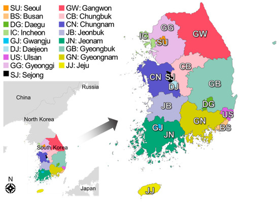
Figure 1.
Administration divisions in Korea [37].
GCAM-Korea exhibits the provincial features of the energy sector. Electricity from coal power plants is mostly generated in Chungnam and Gyeongnam. Electricity is mainly consumed by the building and industrial sectors which are mostly located in the Seoul metropolitan area, Gyeonggi, Chungnam, and Jeonbuk; 77% of the national industrial energy is consumed in four provinces: Jeonam, Chungnam, Ulsan, and Gyeongbuk. Energy consumption in the building and transportation sectors is intensive in the Seoul metropolitan area which accounted for 52% and 44% of the total energy consumption in the building and transportation sectors, respectively, in 2015.
2.2. Modeling Air Pollutant Emissions in GCAM-Korea
As the current GCAM-Korea is modeled only for socioeconomics and energy systems, air pollutant emissions modeling is a new feature which requires to be augmented. Hence, this study further develops GCAM-Korea by using air pollutant emissions data from the national air pollutant emissions inventory.
2.2.1. National Air Pollutant Emissions Inventory
The National Institute of Environmental Research (NIER) provides estimated annual emissions through the Clean Air Policy Support System (CAPSS). The source classification code (SCC) is based on the classification of CORe INventory AIR (CORINAIR) published by the European Environment Agency (EEA), and it is adjusted by NIER to fit Korean activity classifications. The sources of fugitive dust and biomass burning were not included in the annual information till 2015. SCC comprises of 13 large categories—energy production combustion, non-industrial combustion, manufacturing industry, industrial processes, energy transport and storage, solvent use, road transportation, non-road transportation, waste, agriculture, other sources and sinks, fugitive dust, and biomass burning; 56 medium categories; and more than 200 small categories (activity sources) at the district level since 2016. In the national emissions inventory, air pollutants consist of CO, NOx, SOx, TSP, PM10, PM2.5, VOC, NH3, and BC [38,39].
Road transportation is composed of eight vehicles by fuel type (gasoline, LPG, diesel and compressed natural gas (CNG)). The vehicle types are: passenger cars, taxis, vans, buses, freight cars, recreational vehicles, two-wheeled vehicles, and special vehicles. In the emissions inventory, emissions from road transportation are estimated using total vehicle kilometers traveled (VKT), the statistics of total registered motor vehicles, and emission factors by each type of vehicle, fuel, and species [38]. The total VKT is a sum of measured VKT and unmeasured VKT. Measured VKT is calculated using traffic volume and road length by road sections. Unmeasured VKT is estimated using vehicle type, vehicle age, and average driving speed on a district basis. All provinces are assumed to have the same emission factors for each vehicle type and species. Emission factors, however, are known to deteriorate with high driving speed and a vehicle’s age [40].
Fugitive dust in the emissions inventory is composed of eight sub-categories including paved road dust, unpaved road dust, and construction. However, this study only focuses on paved and unpaved road fugitive dust (from now on referred to as FRD). FRD’s estimation is based on total VKT and emission factor for wear (tire wear, brake wear, and road wear). The emission factor for tire and brake wear is calculated using data measured by the mandatory vehicle inspection. The road wear emission factor is calculated using vehicle weight and measured silt loading. Silt loading means resuspended road dust per road surface [41,42].
2.2.2. Applying Air Pollutant Emissions Data in GCAM-Korea
Air pollutant emissions data obtained from the National Air Pollutant Emissions Service [43] was reclassified to match NIER’s activity sources to road transportation modes in GCAM-Korea (see Appendix A), fuels, and provinces in GCAM-Korea; 276 districts excluding Sejong are merged into 16 provinces. Gasoline, LPG, and diesel are aggregated into refined liquids, and CNG is mapped to gas in GCAM-Korea. FRD sources are sub-divided based on their share of energy use that is calculated using the energy consumption survey [44], VKT [45], and fuel efficiency [46] because the sub-classification of FRD sources is aggregated across vehicle type, vehicle size, and fuel type in the emissions inventory. As FRD emissions data for BEVs and FCEVs is currently not available in the emissions inventory, these emissions models are ignored in this study.
The calibration year for GCAM-Korea is 2010. However, emissions data for various years is used for the model’s calibration (see Table 2) on account of missing data or data which contradicts energy use as illustrated in Figure 2.
Table 2.
Year of air pollutant emissions data used for the calibration.
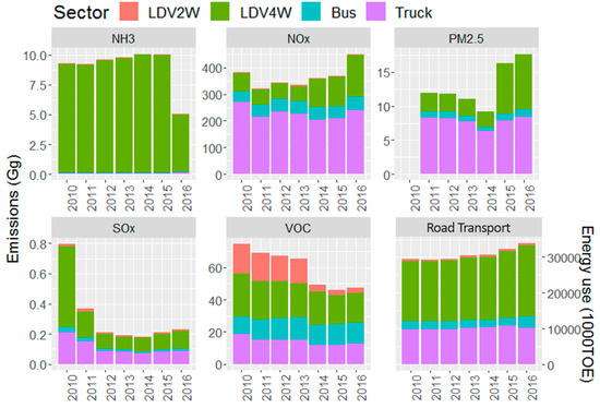
Figure 2.
Reclassified emissions and energy use in road transportation. Note: Total energy use of road transportation is from the energy balance table in the Yearbook of Energy Statistics [44], and the sectoral share [47,48,49] is applied to total energy use.
For example, SOx emissions from light-duty 4-wheel vehicles (LDV4W) were notably high only in 2010, while its energy use increased steadily during the study period. As VKT is closely related to energy use, comparing emissions to energy use instead of VKT is suitable under the assumption that there is no big change of technology development or regulations on SOx emissions. In actual fact, there is no big change. The main reason that the calibration year’s data is not used is for avoiding overestimation or underestimation of future emissions. If SOx emissions in 2010 are used for calibration, future emissions will be overestimated. Another reason for using different years’ emissions data is the absence of data in the calibration year. FRD and PM2.5 emissions from light-duty vehicle 2-wheels (LDV2W) were newly released in 2015 and 2016, respectively.
3. Scenario Design
The ZEVs purchase subsidy is provided for cars (LDV4W) and buses for both BEVs and FCEVs. Subsidy for motorcycles (LDV2W) and freight trucks (less than 1 tonne) is available only for BEVs. Subsidy is provided not only by the national government but also by the local government. Subsidy from the national government is the same everywhere, but subsidy from the local government is different. For example, local government subsidy for LDV4W’s BEVs range from $4100 in Seoul to $10,000 in Ulleung-gun, Gyeongbuk. The national government subsidy for LDV4W is between $5600 and $7500, depending on the vehicle model. On the other hand, local government subsidies for LDV4W’s FCEVs are available only in eight provinces, ranging from $9100 in Incheon to $18,000 in Goseong-gun, Gangwon. The government subsidy for one of the FCEVs, NEXO, manufactured by Hyundai, is $20,500. Note that subsidy for LDV2W, buses, and trucks is equally supported by all local governments. Although the national government offers tax incentives for ZEV buyers, this study considers only the ZEV purchase subsidy.
To apply subsidy to GCAM-Korea, vehicle models are first classified into vehicle types. Then, the average subsidy of each vehicle type is calculated for each province. The calculated subsidy for BEVs and FCEVs is given in Appendix B and Appendix C respectively.
Second, future subsidy scenarios are developed (Table 3). According to CPFDM, subsidy for passenger cars will gradually be phased out, although the exact information on expiration has not been announced. A ‘Sunset’ scenario, therefore, is assumed in which subsidy for only LDV4W’s BEVs will be phased out by 2040. In this scenario, the subsidy declines linearly to zero by 2040. A ‘NoSunset’ scenario is assumed for comparison. In both the scenarios, ZEVs subsidy is available from 2020. For the baseline analysis without any subsidy, a ‘REF’ or a reference case for the projected emissions of the baseline is prepared.
Table 3.
Description of scenarios.
In GCAM-Korea, new technologies such as hydrogen buses, electric buses, and electric freight trucks (less than 1 tonne), have not been modeled yet. Hence, these new technologies are added to the nesting structure of the transportation sector in GCAM-Korea for an analysis (Figure 3). As future technology cost estimations largely depend on the scope of research, a relative cost approach is adopted. Purchase costs are obtained from various sources, and maintenance costs are calculated by applying the ratio of maintenance costs to the present value of purchase costs from previous studies (see Appendix D). Infrastructure costs such as charging stations and hydrogen production facilities are not considered. Future cost trends of electric buses and trucks are assumed based on the decreasing rate of cost of electric passenger cars in GCAM version 5.1.3. Likewise, the trend of hydrogen buses is assumed based on the trend of hydrogen passenger cars in GCAM.
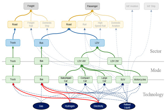
Figure 3.
New nesting structure for the transportation sector in GCAM-Korea. Note: Red line indicates a newly added technology and blurry figures denote non-road transportation sectors.
Finally, the subsidy is subtracted from the total cost of each vehicle technology. According to our calculations, the total cost of an electric bus and a hydrogen bus is about 2.1 times and 4.0 times that of a diesel bus respectively. The total cost of an electric freight truck is about 1.8 times that of a one-tonne diesel truck.
4. Results
4.1. Projected Emissions at the Baseline
Table 4 summarizes projected emissions at the baseline (REF). It compares emissions from GCAM-Korea and those from the national emissions inventory. The projected emissions are captured fairly well in terms of sectors and provinces. The NH3, NOx, PM2.5, SOx, and VOC emissions in 2015 are projected as 80%, 94%, 97%, 81%, and 129% respectively, compared to emissions in the emissions inventory. In REF, the LDV4W and truck sectors are the main contributors to PM2.5 emissions. The truck sector in particular accounted for 71% of NOx emissions while the LDV4W sector accounted for 98% of the total NH3 emissions.
Table 4.
Comparison of emissions from the national inventory and those from GCAM-Korea (2015).
Projected emissions by year and province are given in Figure 4. Sectoral emissions are projected between 72% and 119% compared to emissions in the emissions inventory except for VOC for LDV2W (456%) and NOx for LDV4W (53%). VOC emissions for LDV2W are overestimated because of the abrupt decrease in emissions reported in the national emissions inventory. Its emissions in 2015 (2.96 Gg) fell by 80% as compared to emissions in 2013 (15.25 Gg), whereas energy use for LDV2W increased slightly from 484 KTOE in 2013 to 514 KTOE in 2015. For a similar reason, NOx emissions for LDV4W cannot be captured well. Its emissions in the emissions inventory have dramatically increased since 2014, when it was more than two times the emissions in 2010.
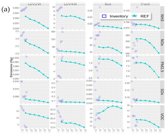
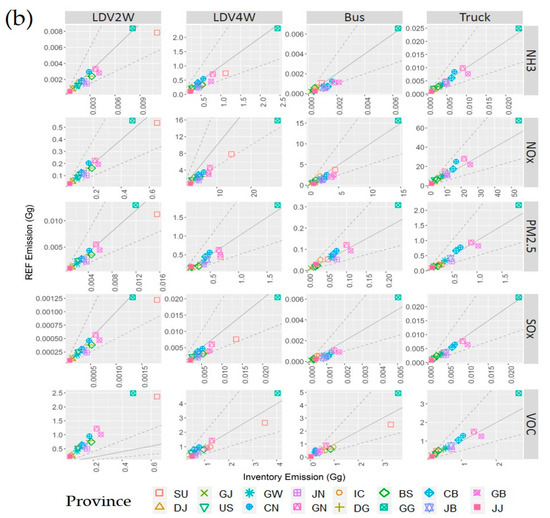
Figure 4.
Projected emissions from the baseline (REF) compared to the national emissions inventory. Note: (a) Trend of the projected emissions and (b) projected emissions by provinces in 2015.
The REF scenario shows that projected emissions in the future are on a downward trajectory because of fuel switching from refined liquids to natural gas (NG), electricity, and hydrogen (see Figure 5b,c). The trends in NOx and PM2.5 emissions for the truck sector show a steeper decline than that for other sectors. The difference in emissions between 2020 and 2040 is 1446 tonnes of PM2.5 and 47,050 tonnes of NOx. The LDV4W sector, a major contributor to NH3 emissions, is expected to reduce 860 tonnes of NH3 emissions from 2020 till 2040.
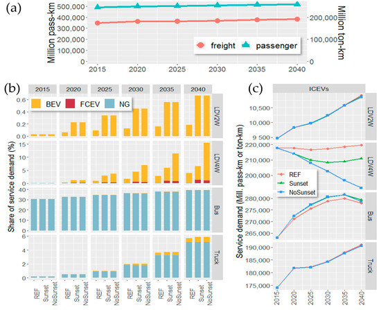
Figure 5.
Service demand in the road transportation sector. Note: Total service demand: (a), Technology share (b), Service demand of ICEVs (c). The rest of the percentage of bars in (b) is the share of service demand for refined liquid vehicles.
As mentioned earlier, Seoul and Gyeonggi, a populous urban area with the highest number of vehicles [50], are expected to have most of the air pollutant emissions from all road transportation sectors. The truck sector in particular produces large emissions in Gyeonggi. In this province, annual VKT of trucks is the highest among all provinces because of the massive road freight volume due to the manufacture of plastics and synthetic rubber [51].
The second most polluted area is Gyeongsang province (Gyeongbuk and Gyeongnam), since this province is the second most populous province next to the Seoul metropolitan area which accounted for 12% of the whole population of South Korea in 2015. In this province, energy consumption by trucks accounted for 16% of the total truck energy consumption, serving a huge industrial complex in this region.
4.2. ZEVs Promotion Using the Subsidy Policy
The ZEV subsidy increases ZEVs’ service demand in all the sectors (Figure 5b) while total transportation service demand is kept almost the same (Figure 5a), showing only around 0.1% difference depending on the scenarios. BEVs’ service demand noticeably increases in the LDV4W sector, since LDV4W is the main target of subsidy support. In the Sunset scenario, the share of service demand for BEVs and FCEVs is expected to be 2.6% and 0.2% respectively in 2025. In 2040, the share of BEVs and FCEVs increases to 5.3% and 1.2% respectively. REF’s share is 0.8% for BEVs and 0.03% for FCEVs in 2040. The share for BEVs rises further to 14.4% in 2040 if the current subsidy is maintained till 2040 (the NoSunset case), while the share of FCEVs starts decreasing to around 1% despite the same amount of subsidy. Even if FCEVs receive the same subsidy, their market entry is disturbed by the introduction of BEVs considering the total service demand, which does not change significantly.
On the other hand, other vehicles excluding LDV4W, show minor effects on service demand change. As NG vehicles dominate service demand in the truck and bus sectors, ZEVs’ share is less than 1% even in 2040. Besides, ICEVs’ service demand increases in the bus sector with the ZEV subsidy, that is, there are intensive share increases in ZEVs’ share in the LDV4W sector leading to an increase in its service demand and average service costs at the same time, while bus service costs become relatively cheaper. The reason for the increase in LDV4W sector’s service costs is high-cost technologies (BEVs and FCEVs) being introduced in this sector. In 2040, the relative service cost of the bus sector is 0.80 in the Sunset case and 0.81 in the NoSunset case based on the LDV service cost of 1. By the price response, bus service demand increases by 0.3–0.7% compared to REF and increases further in the Sunset case (Figure 5c).
Demand for electricity and hydrogen increases with the growth of BEVs and FCEVs’ service demands. In the Sunset case, electricity demand increases from 9.7PJ (REF case) to 12.2PJ in 2025, and from 16.1PJ (REF case) to 18.8PJ in 2040. In the NoSunset case, it further increases to 13.2PJ in 2025 and 31.3PJ in 2040. In the case of hydrogen demand, while the REF case shows the demand at 0.05PJ even in 2040, demands increases to 0.4PJ in 2025 and 2.3PJ in 2040 in the Sunset case. The NoSunset case shows the demand decreasing rather than increasing as compared to the Sunset case, which is 0.4PJ in 2025 and 1.9PJ in 2040, because of a decrease in FCEVs’ service demand. Changes in the prices of electricity and hydrogen are negligible ranging between 0.0% and 0.3% during the period.
Figure 6 shows the estimates of a cumulative number of ZEVs and a comparison with the government’s target for ZEV promotion. According to CPFDM, the goal is to have 850,000 BEVs and 150,000 FCEVs by 2024. In the Sunset case, the total number of vehicles is estimated to be approximately 313,000 BEVs and 22,000 FCEVs in 2025. BEVs and FCEVs are expected to be 3 times and 44 times more than the REF case respectively. In the NoSunset case, it is estimated at 399,000 BEVs and 21,000 FCEVs, which is a 22% increase and 3% decrease respectively compared to the Sunset case. But both scenarios fail to achieve the government’s target of ZEV promotion.
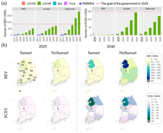
Figure 6.
Estimates of the cumulative number of ZEVs by sector (a) and by province (b).
In the Seoul metropolitan area, the cumulative number of BEVs is estimated at 128,000 in 2025, which accounts for 41% of the total BEVs. In 2040, BEVs in this area are estimated at 307,000 in the Sunset case and 738,000 in the NoSunset case. FCEVs are mostly promoted in provinces where local subsidies are provided and not in the Seoul metropolitan area. Accordingly, Gangwon, where the largest subsidy for FCEVs is provided, is the second most diffused province. In Gangwon, the estimated number of FCEVs is 2900 in 2025 in the Sunset scenario. Chungnam and Gyeongnam follow with 1900 FCEVs each.
Table 5 summarizes the required subsidy for meeting the ZEVs scenarios from 2020 to 2040. It is estimated that total subsidy required during the period will be approximately $9.6 billion in the Sunset case and $24.7 billion in the NoSunset case. Above all, around 90% of the total subsidy spending is concentrated in the LDV4W sector.
Table 5.
Required subsidy by scenarios (unit: Million $).
4.3. Effects of ZEV Promotion on Air Pollution
As shown in Figure 7, most emission reductions are expected from the LDV4W sector because ZEVs’ dissemination is mostly expected in this sector. In general, emissions slightly reduce for all pollutants. In the Sunset case, emission reduction rates of NH3, NOx, PM2.5, SOx, and VOC are expected to be 3.7% (254 tonnes), 0.5% (1488 tonnes), 1.2% (155 tonnes), 1.5% (2 tonnes), and 0.9% (462 tonnes) respectively in 2040. In the NoSunset case, the NH3 emission reduction rate is expected to be relatively higher due to the increase in ZEVs’ share in the LDV4W sector—the LDV4W sector has high NH3 emissions. On the other hand, emissions from the bus sector rise for all pollutants compared to REF with an increase in its service demand (Figure 5c). Estimates of PM2.5 emission reduction are smaller than autonomously reduced emissions over time without any policy (the REF case).
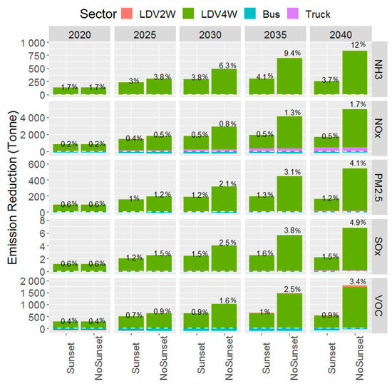
Figure 7.
Emission reductions compared to emissions in REF (each scenario minus REF). Note: The values above the bars represent the percentage of emission reductions compared to REF.
According to CPFDM, the government has set a target of reducing NOx, PM2.5, SOx, and VOC emissions in the transportation sector by 65%, 36%, 71%, and 44% of the emissions in 2024 respectively below those in 2016. In case of NH3, there is no reduction target for the transportation sector. To compare the simulation results, the emission reduction target in the transportation sector is divided into emissions targets for the road transportation sector and the non-road transportation sector according to their proportion in base year 2016. As the simulation results are represented in a 5-year step, projected emissions are linearly interpolated.
Table 6 gives a comparison of the simulation results for emission reduction targets for the road transportation sector. The SOx emission reduction target can be seen to be intended for the non-road transportation sectors considering the SOx emissions portion in road transportation (0.6%). The simulation results show that NOx, PM2.5, and VOC emission reduction targets can be achieved as much as 4.0%, 11.5%, and 4.8% respectively in the Sunset case. According to a report released by the National Assembly Budget Office [10], the ZEV subsidy policy does not have a significant impact on reducing PM2.5. PM2.5 emission reductions by the ZEV subsidy policy accounted for only 3% of the overall emission reductions by PM2.5 mitigation measures for the road transportation sector, whereas 76% of the overall budget for them was spent on the ZEVs subsidy in 2018 according to the report.
Table 6.
Expected emission reductions in 2024 compared to 2016.
Figure 8 illustrates expected emission reductions by province. The pattern of emission reductions is similar to expected ZEVs’ dissemination (Figure 6b). For example, the Seoul metropolitan area has the highest transportation activities, showing the biggest emission reductions in all the scenarios. In the Sunset scenario, the emission reductions expected in 2040 are 130 tonnes of NH3 (51% of national emission reductions); 711 tonnes of NOx (48%); 68 tonnes of PM2.5 (44%); 1 tonne of SOx (50% ); and 244 tonnes of VOC (53%). Chungnam and Chungbuk, which provide the highest subsidy for BEVs in LDV4W, show the second and third-largest emission reductions, following the Seoul metropolitan area. The expected emission reductions in these two provinces are 40 tonnes of NH3 (16%), 238 tonnes of NOx (16%), 32 tonnes of PM2.5 (21%), 0.3 tonnes of SOx (15%), and 57 tonnes of VOC (12%) in the Sunset case.
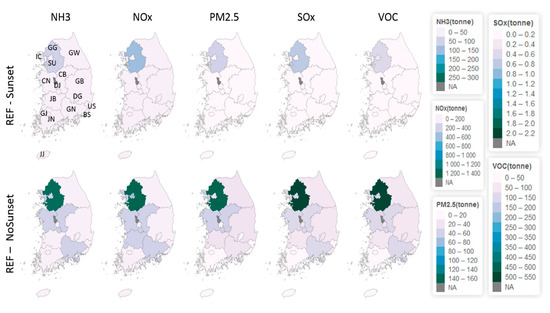
Figure 8.
Emission reductions compared to REF in 2040.
5. Conclusions and Policy Implications
This study modeled air pollutant emissions using GCAM-Korea focusing on the road transportation sector. The projected emissions compared to the national emissions inventory using GCAM-Korea works fairly well with empirical data across sectors and provinces except for VOC from LDV2W in which the reported emissions in the emissions inventory contradict energy use.
The study applied the extended GCAM-Korea with air pollutant emissions modeling for examining the ZEV subsidy’s effects on emission reductions for PM2.5 as well as its precursors. Subsidy scenarios based on the current policy are found to have a major impact on the LDV4W sector in terms of change in service demand and emission reduction, whereas it is expected to have a minor impact on the other sectors. In all the scenarios, the government’s target of ZEVs’ dissemination is expected to be not attainable. The resulting expected emission reductions of PM2.5 are 0.6–1.2% in the Sunset case and 0.6–4.1% in the NoSunset case compared to the baseline. The Seoul metropolitan area contributes 38–44% of the total emission reductions. Chungcheong province is the second most mitigated province next to the Seoul metropolitan area because of the second and third largest subsidy for BEVs in the LDV4W sector, even though this province has relatively low traffic and a small population compared to metropolitan areas. Its emission reduction accounts for 17–21% and 17–20% of the overall emission reductions in the Sunset and the NoSunset cases respectively. NH3 is the most mitigated pollutant, for which the emission reduction rate is 1.7–3.7% in the Sunset case and 1.7–12% in the NoSunset case. On the other hand, NOx emissions are expected to reduce very slightly with an emission reduction rate of 0.2–0.5% and 0.2–1.7% in the Sunset and NoSunset cases respectively.
As the ZEVs subsidy is weighted towards the LDV4W sector, as is shown in Table 5, various spillover effects are found: ZEVs’ share rises intensively in the LDV4W sector, which leads to an increase in its service costs, while this drives the bus service costs to become relatively cheaper. This whole process, in turn, drives an increase in bus service demand and emissions. In other words, an imbalanced ZEVs subsidy distribution may dampen the subsidy’s effect on air pollution improvements. Furthermore, the ZEVs subsidy is not expected to reduce ICEVs in the truck sector, although diesel freight trucks are a major contributor to PM2.5 emissions as also NOx. This means targeting emission reduction by promoting ZEVs might be misleading without explicit consideration of ICEVs in the truck sector. Another finding is that the decline in emissions over time without any policy is more than the ZEV subsidy’s effects.
As this analysis does not cover uncertainty in the total costs of ZEVs, this should be considered in a future study. While infrastructure costs increase ZEVs’ total costs, incentives for charging station installations and tax incentives for buyers decrease costs. Moreover, total costs can vary under future trends of efficiency and costs. The amount of ZEV purchase subsidy for the future is also uncertain because the government has not decided on this as yet. The uncertainty around cost eventually influences ZEVs’ service demand, which changes the effects of the ZEV subsidy policy on air quality mitigation. In addition, emissions caused by increasing electricity and hydrogen consumption for ZEVs should also be considered from the perspective of the entire energy system. Emissions modeling for other sectors such as power generation and industry sectors will be conducted which is expected to provide more meaningful implications for cross-sector and cross-province aspects in the future.
Author Contributions
Conceptualization, M.R., S.J., S.K. (Suduk Kim), S.K. (Soontae Kim), and S.Y.; Methodology, M.R. and S.J.; Software, M.R. and S.J.; Data curation, M.R. and S.J.; Visualization, M.R.; Writing—Original Draft Preparation, M.R.; Writing—Review & Editing, S.K. (Suduk Kim), S.Y., S.K. (Soontae Kim) and A.H.; Supervision, S.K. (Suduk Kim); Funding acquisition, S.K. (Suduk Kim). All authors have read and agreed to the published version of the manuscript.
Funding
This work was supported by the Technology Development Program to Solve Climate Changes of the National Research Foundation (NRF) funded by the Ministry of Science, ICT & Future Planning (NRF-2017M1A2A2081253), and the Korea Ministry of Environment (MOE) as Graduate School specialized in Climate Change.
Acknowledgments
We would like to thank Jaeick Oh, Jaesung Jung, and three anonumous reviewers for their valuable comments.
Conflicts of Interest
The authors declare no conflict of interest.
Appendix A
Table A1.
The Mapping of Vehicle Type in the National Inventory to Vehicle Mode in GCAM-Korea.
Table A1.
The Mapping of Vehicle Type in the National Inventory to Vehicle Mode in GCAM-Korea.
| Classification of National Emissions Inventory | GCAM-Korea | |
|---|---|---|
| Medium Category | Small Category | Mode |
| Passenger car | Compact | Subcompact Car |
| Passenger car | Small | Subcompact Car |
| Passenger car | Medium | Compact Car |
| Passenger car | Large | Large Car |
| Taxi | Medium | Compact Car |
| Taxi | Large | Large Car |
| Van | Compact | Bus |
| Van | Small | Bus |
| Van | Medium | Bus |
| Van | Large | Bus |
| Van | Special purpose | Bus |
| Bus | Chartered bus | Bus |
| Bus | City bus | Bus |
| Bus | Intercity bus | Bus |
| Bus | Express bus | Bus |
| Freight car | Compact | Truck |
| Freight car | Small | Truck |
| Freight car | Medium | Truck |
| Freight car | Large | Truck |
| Freight car | Special purpose | Truck |
| Freight car | Dump truck | Truck |
| Special vehicle (SV) | Recovery vehicle | Truck |
| Special vehicle (SV) | Wrecker car | Truck |
| Special vehicle (SV) | Others | Truck |
| Recreational vehicle (RV) | Small | Light Truck and SUV |
| Recreational vehicle (RV) | Medium | Light Truck and SUV |
| Two-wheeled vehicle | Less than 50 cc | Motorcycle |
| Two-wheeled vehicle | 50 cc~99 cc | Motorcycle |
| Two-wheeled vehicle | 100 cc~259 cc | Motorcycle |
| Two-wheeled vehicle | More than 260 cc | Motorcycle |
Appendix B
Table A2.
Average Subsidy for Battery Electric Vehicles by Province in 2020 (Unit: Thous.$).
Table A2.
Average Subsidy for Battery Electric Vehicles by Province in 2020 (Unit: Thous.$).
| Province | LDV2W | LDV4W | Bus | Truck | |||
|---|---|---|---|---|---|---|---|
| Motor-Cycle | Subcompact | Compact | Large | SUV | |||
| SU | 2.1 | 6.2 | 10.8 | 10.7 | 11.5 | 74.9 | 15.5 |
| IC | 2.1 | 6.1 | 11.9 | 11.8 | 12.7 | 74.9 | 14.6 |
| DJ | 2.1 | 6.4 | 13.0 | 12.8 | 13.8 | 74.9 | 15.2 |
| DG | 2.1 | 5.5 | 11.3 | 11.1 | 12.0 | 74.9 | 13.9 |
| GJ | 2.1 | 5.9 | 11.9 | 11.8 | 12.7 | 74.9 | 13.7 |
| BS | 2.1 | 6.4 | 11.3 | 11.1 | 12.0 | 74.9 | 14.1 |
| US | 2.1 | 6.4 | 12.1 | 12.0 | 12.9 | 74.9 | 21.8 |
| GG | 2.1 | 5.9 | 11.3 | 11.2 | 12.0 | 74.9 | 15.3 |
| GW | 2.1 | 6.4 | 12.8 | 12.7 | 13.6 | 74.9 | 18.7 |
| CB | 2.1 | 8.1 | 13.8 | 13.7 | 14.7 | 74.9 | 23.2 |
| CN | 2.1 | 7.0 | 13.7 | 13.5 | 14.6 | 74.9 | 20.0 |
| JB | 2.1 | 5.9 | 14.7 | 14.5 | 15.6 | 74.9 | 18.4 |
| JN | 2.1 | 6.0 | 13.6 | 13.4 | 14.5 | 74.9 | 23.4 |
| GB | 2.1 | 6.4 | 12.3 | 12.1 | 13.1 | 74.9 | 19.2 |
| GN | 2.1 | 5.6 | 12.5 | 12.3 | 13.3 | 74.9 | 18.7 |
| JJ | 2.1 | 7.3 | 11.3 | 11.1 | 12.0 | 74.9 | 15.2 |
Note: The subsidy is calculated based on information obtained from [52].
Appendix C
Table A3.
Average Subsidy for Fuel Cell Electric Vehicles by Province in 2020 (Unit: Thous.$).
Table A3.
Average Subsidy for Fuel Cell Electric Vehicles by Province in 2020 (Unit: Thous.$).
| Province | LDV2W | LDV4W | Bus | Truck | |||
|---|---|---|---|---|---|---|---|
| Motor-Cycle | Subcompact | Compact | Large | SUV | |||
| SU | - | 20.5 | 20.5 | 20.5 | - | 136.4 | - |
| IC | - | 15.8 | 29.5 | 29.5 | - | 136.4 | - |
| DJ | - | 20.5 | 20.5 | 20.5 | - | 136.4 | - |
| DG | - | 20.5 | 20.5 | 20.5 | - | 136.4 | - |
| GJ | - | 20.5 | 20.5 | 20.5 | - | 136.4 | - |
| BS | - | 16.8 | 31.4 | 31.4 | - | 136.4 | - |
| US | - | 20.5 | 20.5 | 20.5 | - | 136.4 | - |
| GG | - | 15.8 | 29.5 | 29.5 | - | 136.4 | - |
| GW | - | 20.6 | 38.6 | 38.6 | - | 136.4 | - |
| CB | - | 15.8 | 29.5 | 29.5 | - | 136.4 | - |
| CN | - | 16.6 | 31.1 | 31.1 | - | 136.4 | - |
| JB | - | 20.5 | 20.5 | 20.5 | - | 136.4 | - |
| JN | - | 17.0 | 31.8 | 31.8 | - | 136.4 | - |
| GB | - | 20.5 | 20.5 | 20.5 | - | 136.4 | - |
| GN | - | 16.1 | 30.1 | 30.1 | - | 136.4 | - |
| JJ | - | 20.5 | 20.5 | 20.5 | - | 136.4 | - |
Note: The subsidy is calculated based on information obtained from [52].
Appendix D
Table A4.
Assumptions for an Electric Truck, Electric Bus, and Hydrogen Bus.
Table A4.
Assumptions for an Electric Truck, Electric Bus, and Hydrogen Bus.
| Sector | Bus | Truck | |||
|---|---|---|---|---|---|
| Fuel Type | Electricity | Hydrogen | CNG | Electricity | Diesel |
| Fuel intensity (MJ/VKT) | 5.3 1 | 12.9 1 | 5.8 1 | 1.2 2 | 1.5 2 |
| Purchase cost ($/vehicle) | 408,500 3 | 83,000 4 | 168,290 5 | 50,000 2 | 20,000 6 |
| VKT 2 (miles/vehicle-year) | 34,053 | 34,053 | 34,053 | 13,116 | 13,116 |
| Lifetime 2 (year) | 8 | 8 | 8 | 8 | 8 |
| Non-energy cost ($/VKT) | 0.23 1 | 0.22 1 | 0.26 1 | 0.1 2 | 0.17 2 |
| Total cost ($/VKT-year) | 2.48 | 4.78 | 1.18 | 0.815 | 0.456 |
| Relative price | 2.1 | 4.0 | 1 | 1.8 | 1 |
Note: A 10% the discount rate is applied for calculating the present value of future vehicle purchase costs. 1 Eudy et al. [53]; 2 Dana incorporated [54]; 3 Edison motors [55]; 4 Ministry of Environment [56]; 5 Daewoo bus [57]; and 6 Kia motors [58].
References
- Trnka, D. Policies, Regulatory Framework and Enforcement for Air Quality Management: The Case of Korea; OECD: Paris, France, 2020; pp. 12–22. [Google Scholar] [CrossRef]
- World Health Organization (WHO). Health Effects of Particulate Matter. Policy Implications for Countries in Eastern Europe, Caucasus and Central Asia; WHO: Copenhagen, Denmark, 2013; pp. 6–7. Available online: https://www.euro.who.int/__data/assets/pdf_file/0006/189051/Health-effects-of-particulate-matter-final-Eng.pdf?ua=1 (accessed on 20 March 2020).
- Han, C.; Kim, S.; Lim, Y.; Bae, H.; Hong, Y. Spatial and temporal trends of number of deaths attributable to ambient PM2.5 in the Korea. J. Korean Med. Sci. 2018, 33, e193. [Google Scholar] [CrossRef]
- National Institute of Environmental Research (NIER). Sourcebook of PM2.5 Emission Factor; NIER: Incheon, Korea, 2014; pp. 1–2. Available online: http://webbook.me.go.kr/DLi-File/NIER/09/019/5568844.pdf (accessed on 15 October 2019).
- Ministry of Land, Infrastructure and Transport (MOLIT). Status of the Metropolitan Area and Provincial Area. Available online: http://www.index.go.kr/potal/main/EachDtlPageDetail.do?idx_cd=2729 (accessed on 19 March 2020).
- Ministry of Environment (MOE). 2017 White Paper of Environment; MOE: Sejong, Korea, 2017; pp. 126–128. Available online: http://webbook.me.go.kr/DLi-File/091/025/006/5636222.pdf (accessed on 18 March 2020).
- Pan-government. Comprehensive Plan on Fine Dust Management (2020–2024); Pan-government: Korea, 2019. Available online: https://www.me.go.kr/home/file/readDownloadFile.do?fileId=168738&fileSeq=5 (accessed on 21 April 2020).
- NIER. Air Pollutants Emission Statistics in 2016. Available online: https://airemiss.nier.go.kr/common/downLoad.do?siteId=airemiss&fileSeq=512 (accessed on 17 February 2020).
- Lutsey, Nic. Transition to a Global Zero-Emission Vehicle Fleet: A Collaborative Agenda for Governments; International Council on Clean Transportation: Washington DC, USA, 2015; pp. 1–2. Available online: http://theicct.org/sites/default/files/publications/ICCT_GlobalZEVAlliance_201509.pdf (accessed on 24 May 2020).
- National Assembly Budget Office (NABO). Analysis of Projects about Particulate Matter Measure; NABO: Seoul, Korea, 2019; pp. 17–20. Available online: https://www.nabo.go.kr/system/common/JSPservlet/download.jsp?fCode=33315609&fSHC=&fName=%EB%AF%B8%EC%84%B8%EB%A8%BC%EC%A7%80+%EB%8C%80%EC%9D%91+%EC%82%AC%EC%97%85+%EB%B6%84%EC%84%9D.pdf&fMime=application/pdf&fBid=19&flag=bluene (accessed on 1 April 2020).
- Ministry of Trand, Industry and Energy (MOTIE). Road Map for Regulatory Preemption of Eco-Friendly Vehicles. Available online: http://www.motie.go.kr/common/download.do?fid=bbs&bbs_cd_n=81&bbs_seq_n=162871&file_seq_n=1 (accessed on 22 July 2020).
- EV. Support for Charging Station Installation. Available online: https://www.ev.or.kr/portal/buyersGuide/slowInstallSupport?pMENUMST_ID=21628 (accessed on 22 July 2020).
- Kriegler, E.; Petermann, N.; Krey, V.; Schwanitz, V.J.; Luderer, G.; Ashina, S.; Bosetti, V.; Eom, J.; Kitous, A.; Mejean, A.; et al. Diagnostic indicators for integrated assessment models of climate policy. Technol. Forecast. Soc. Chang. 2015, 90, 45–61. [Google Scholar] [CrossRef]
- Kim, B.; Lee, W.; Jo, H.; Lee, B. Making primary policies for reducing particulate matter. J. Soc. E-Bus. Stud. 2020, 25, 109–121. [Google Scholar] [CrossRef]
- Kim, E.; Kim, H.; Kim, B.; Kim, S. PM2.5 Simulations for the Seoul Metropolitan Area: (VI) Estimating Influence of Sectoral Emissions from Chumngcheongnam-do. J. Korean Soc. Atmos. Environ. 2019, 35, 226–248. [Google Scholar] [CrossRef]
- Kim, H.; Kim, S.; Lee, S.; Kim, B.; Lee, P. Fine-Scale Columnar and Surface NOx Concentrations over South Korea: Comparison of Surface Monitors, TROPOMI, CMAQ and CAPSS Inventory. Atmosphere 2020, 11, 101. [Google Scholar] [CrossRef]
- Kim, O.; Bae, M.; Kim, S. Evaluation on Provincial NOx and SO2 Emission in CAPSS 2016 Based on Photochemical Model Simulation. J. Korean Soc. Atmos. Environ. 2020, 36, 64–82. [Google Scholar] [CrossRef]
- Shi, W.; Ou, Y.; Smith, S.J.; Ledna, C.M.; Nolte, C.G.; Loughlin, D.H. Projecting state-level air pollutant emissions using an integrated assessment model: GCAM-USA. Appl. Energy 2017, 208, 511–521. [Google Scholar] [CrossRef] [PubMed]
- Jeon, H.; Lee, H. Valuing Air Pollution Using the Life Satisfaction Approach; Korea’s Allied Economic Associations Annual Meeting: Sejong, Korea, 2019; pp. 139–154. Available online: http://210.101.116.28/W_files/kiss6/33001315_pv.pdf (accessed on 23 March 2020).
- Ou, Y.; West, J.J.; Smith, S.J.; Nolte, C.G.; Loughlin, D.H. Air pollution control strategies directly limiting national health damages in the US. Nat. Commun. 2020, 11, 1–11. [Google Scholar] [CrossRef] [PubMed]
- Amann, M.; Johansson, M.; Lükewille, A.; Schöpp, W.; Apsimon, H.; Warren, R.; Warren, R.; Gonzales, T.; Tsyro, S. An integrated assessment model for fine particulate matter in Europe. Water Air Soil Pollut. 2001, 130, 223–228. [Google Scholar] [CrossRef]
- Loughlin, D.H.; Benjey, W.G.; Nolte, C.G. ESP v1. 0: Methodology for exploring emission impacts of future scenarios in the United States. Geosci. Model Dev. 2011, 4, 287–297. [Google Scholar] [CrossRef]
- Klimont, Z.; Kupiainen, K.; Heyes, C.; Purohit, P.; Cofala, J.; Rafaj, P.; Borken-Kleefeld, J.; Schöpp, W. Global anthropogenic emissions of particulate matter including black carbon. Atmos. Chem. Phys. Discuss. 2017, 17, 8681–8723. [Google Scholar] [CrossRef]
- Zhang, S.; Worrell, E.; Crijns-Graus, W. Mapping and modeling multiple benefits of energy efficiency and emission mitigation in China’s cement industry at the provincial level. Appl. Energy 2015, 155, 35–58. [Google Scholar] [CrossRef]
- Joint Global Change Research Institute (JGCRI). GCAM v5.2 Documentation: Global Change Assessment Model (GCAM). Available online: http://jgcri.github.io/gcam-doc/index.html (accessed on 25 March 2020).
- Edmonds, J.; Wise, M.; Pitcher, H.; Richels, R.; Wigley, T.; MacCracken, C. An integrated assessment of climate change and the accelerated introduction of advanced energy technologies-an application of MiniCAM 1.0. Mitig. Adapt. Strateg. Glob. Chang. 1997, 1, 311–339. [Google Scholar] [CrossRef]
- Kim, S.; Edmonds, J.; Lurz, J.; Smith, S.J.; Wise, M. The ObjECTS framework for integrated assessment: Hybrid modeling of transportation. Energy J. 2006, 27, 63–91. [Google Scholar] [CrossRef]
- McFadden, D. Conditional logit analysis of qualitative choice behavior. In Frontiers in Econometrics; Zarembka, P., Ed.; Academic Press: New York, NY, USA, 1973; pp. 105–142. Available online: https://eml.berkeley.edu/reprints/mcfadden/zarembka.pdf (accessed on 16 May 2020).
- Brenkert, A.L.; Smith, A.J.; Kim, S.H.; Pitcher, H.M. Model. Documentation for the MiniCAM.; Pacific Northwest National Laboratory: Richland, WA, USA, 2003. [Google Scholar]
- Keepin, B.; Wynne, B. Technical analysis of IIASA energy scenarios. Nature 1984, 312, 691–695. [Google Scholar] [CrossRef]
- Loulou, R.; Goldstein, G.; Noble, K. Documentation for the MARKAL Family of Models. October 2004, pp. 65–73. Available online: http://iea-etsap.org/MrklDoc-I_StdMARKAL.pdf (accessed on 16 May 2020).
- Smith, S.J.; Pitcher, H.; Wigley, T.M.L. Future sulfur dioxide emissions. Clim. Chang. 2005, 73, 267–318. [Google Scholar] [CrossRef]
- Yurnaidi, Z.; Kim, S. Reducing Biomass Utilization in the Ethiopia Energy System: A National Modeling Analysis. Energies 2018, 11, 1745. [Google Scholar] [CrossRef]
- Yu, S.; Tan, Q.; Evans, M.; Kyle, P.; Vu, L.; Patel, P.L. Improving building energy efficiency in India: State-level analysis of building energy efficiency policies. Energy Policy 2017, 110, 331–341. [Google Scholar] [CrossRef]
- Yu, S.; Horing, J.; Liu, Q.; Dahowski, R.; Davidson, C.; Edmonds, J.; Liu, B.; Mcjeon, H.; McLeod, J.; Patel, P.; et al. CCUS in China’s mitigation strategy: Insights from integrated assessment modeling. Int. J. Greenh. Gas Control 2019, 84, 204–218. [Google Scholar] [CrossRef]
- Yu, S.; Yarlagadda, B.; Siegel, J.E.; Zhou, S.; Kim, S. The role of nuclear in China’s energy future: Insights from integrated assessment. Energy Policy 2020, 139, 111344. [Google Scholar] [CrossRef]
- Jeon, S.; Roh, M.; Oh, J.; Kim, S. Development of an Integrated Assessment Model at Provincial Level: GCAM-Korea. Energies 2020, 13, 2565. [Google Scholar] [CrossRef]
- NIER. National Air Pollutants Emission in 2016; NIER: Incheon, Korea, 2018; Available online: https://airemiss.nier.go.kr/user/boardList.do?command=view&page=1&boardId=74&boardSeq=526&id=airemiss_040100000000 (accessed on 17 February 2020).
- Yeo, S.; Lee, H.; Choi, S.; Seol, S.; Jin, H.; Yoo, C.; Lim, J.; Kim, J. Analysis of the National Air Pollutant Emission Inventory (CAPSS 2015) and the Major Cause of Change in Republic of Korea. Asian J. Atmos. Environ. 2019, 13, 212–231. [Google Scholar] [CrossRef]
- Ahn, S.J.; Kim, L.; Kwon, O. Korea’s social dynamics towards power supply and air pollution caused by electric vehicle diffusion. J. Clean. Prod. 2018, 205, 1042–1068. [Google Scholar] [CrossRef]
- NIER. Improvement of Methodology of Fugitive Dust Estimation and Development of Real-Time Road Fugitive Dust Measurement Method; Inha University: Incheon, Korea, 2008; Available online: http://www.prism.go.kr/homepage/entire/retrieveEntireDetail.do;jsessionid=FD36972EFA936BA01CFCBEF3889EFBFF.node02?cond_research_name=&cond_research_start_date=&cond_research_end_date=&research_id=1480000-200800517&pageIndex=2833&leftMenuLevel=160 (accessed on 30 March 2020).
- Han, S.; Youn, J.; Jung, Y. Characterization of PM10 and PM2.5 source profiles for resuspended road dust collected using mobile sampling methodology. Atmos. Environ. 2011, 45, 3343–3351. [Google Scholar] [CrossRef]
- NIER. National Air Pollutants Emission Service. Available online: https://airemiss.nier.go.kr/user/boardList.do?handle=160&siteId=airemiss&id=airemiss_030500000000 (accessed on 17 February 2020).
- Korea Energy Economics Institute (KEEI). 2017 Energy Consumption Survey; KEEI: Ulsan, Korea, 2017; Available online: http://www.keei.re.kr/keei/download/YES2017.pdf (accessed on 18 February 2020).
- Korea Transportation Safety Authority (TS). 2016 Average Mileage of Automobile; TS: Gyeongsangbuk-do, Korea, 2017; pp. 32–46. Available online: http://stat.molit.go.kr/portal/common/downLoadFile.do (accessed on 17 February 2020).
- Korea Energy Management Corporation (KEMCO). Development of Pool of Greenhouse Gas Reduction Means in Building and Transport Sector; Korea Institute of Civil Engineering and Building Technology (KICT): Ulsan, Korea, 2013; pp. 32–46. Available online: http://www.kemco.or.kr/web/kem_home_new/_common/ac_downFile.asp?f_name=%5B%uCD5C%uC885%uBCF4%uACE0%uC11C%5D%uAC74%uBB3C%uC218%uC1A1%uBD80%uBB38%20%uC628%uC2E4%uAC00%uC2A4%20%uAC10%uCD95%uC218%uB2E8%20Pool%uAD6C%uCD95.pdf&cc=1466 (accessed on 17 February 2020).
- KEEI. The 11th Edition (2011) Energy Consumption Survey; KEEI: Ulsan, Korea, 2012; Available online: http://www.keei.re.kr/keei/download/ECS2011_Revised.pdf (accessed on 17 February 2020).
- KEEI. The 12th Edition (2014) Energy Consumption Survey; KEEI: Ulsan, Korea, 2015; Available online: http://www.keei.re.kr/keei/download/ECS2014.pdf (accessed on 17 February 2020).
- KEEI. 2017 Energy Consumption Survey; KEEI: Ulsan, Korea, 2018; Available online: http://www.keei.re.kr/keei/download/ECS2017.pdf (accessed on 17 February 2020).
- MOLIT. Total Registered Motor Vehicles. Available online: http://stat.molit.go.kr/portal/cate/statFileView.do?hRsId=58&hFormId=1242&hSelectId=1242&hPoint=001&hAppr=1&hDivEng=&oFileName=&rFileName=&midpath=&month_yn=N&sFormId=1242&sStart=202001&sEnd=202001&sStyleNum=809 (accessed on 21 February 2020).
- Korea Transport Database (KTDB). Freight in Korea; KTDB: Gyeonggi-do, Korea, 2012; Available online: https://www.ktdb.go.kr/www/selectPblcteWebView.do?key=40&pblcteNo=27&searchLclasCode=PBL04 (accessed on 6 April 2020).
- EV. Purchase Subsidies. Available online: https://www.ev.or.kr/portal/localInfo?pMENUMST_ID=21637 (accessed on 10 March 2020).
- Eudy, L.; Post, M. Fuel Cell Buses in U.S. Transit Fleets: Current Status 2018; National Renewable Energy Laboratory (NREL): Golden, CO, USA, 2018. Available online: https://www.nrel.gov/docs/fy19osti/72208.pdf (accessed on 29 February 2020).
- Dana Incorporated. TCO Calculator. Available online: https://apps.dana.com/commercial-vehicles/tco/ (accessed on 12 March 2020).
- Edison Motors. eFIBIRD Purchase Cost. Available online: http://www.edisonmotorsev.com/service/order1 (accessed on 12 March 2020).
- Ministry of Environment (MOE). Press Release; The Pilot Project of a Hydrogen City Bus Will be Undertaken at Six Cities. Available online: http://www.me.go.kr/home/web/board/read.do?boardMasterId=1&boardId=920200&menuId=286 (accessed on 12 March 2020).
- Daewoo Bus. Bus Price Catalog. Available online: http://www.daewoobus.co.kr/newsite/KR/showroom/BusPrice_20170308.pdf (accessed on 12 March 2020).
- Kia Motors. Fuel Efficiency and Purchase Cost of Bongo III EV. Available online: https://www.kia.com/kr/shopping-tools/catalog-price.html (accessed on 12 March 2020).


© 2020 by the authors. Licensee MDPI, Basel, Switzerland. This article is an open access article distributed under the terms and conditions of the Creative Commons Attribution (CC BY) license (http://creativecommons.org/licenses/by/4.0/).