Abstract
The electrical sector needs to study how energy demand changes to plan the maintenance and purchase of energy assets properly. Prediction studies for energy demand require a high level of reliability since a deviation in the forecasting demand could affect operation costs. This paper proposed a short-term forecasting energy demand methodology based on hierarchical clustering using Dynamic Time Warp as a similarity measure integrated with Artificial Neural Networks. Clustering was used to build the typical curve for each type of day, while Artificial Neural Networks handled the weather sensibility to correct a preliminary forecasting curve obtained in the clustering stage. A statistical analysis was carried out to identify those significant factors in the prediction model of energy demand. The performance of this proposed model was measured through the Mean Absolute Percentage Error (MAPE). The experimental results show that the three-stage methodology was able to improve the MAPE, reaching values as good as 2%.
1. Introduction
Energy demand forecasting is a topic that is drawing interest in electricity market agents (e.g., regulation and distribution companies), providing valuable information for conducting reliability studies in the electric power systems (EPS). For example, demand forecasting studies help to establish the levels of chargeability in circuits, electrical bars and transformers properly. The changing nature in the energy demand due to external factors such as weather conditions can increase the uncertainty when planning increasing the operation costs in the electricity market.
However, the energy demand has a dynamic behaviour which is dependent on several factors such as world population increase, weather-conditions variability and the evolution of EPS architectures (for example, due to renewable energy sources and distributed generation), among other factors. In particular, modified EPS schemes also require the development of new models that consider a more stochastic operation for improved reliability. Such prediction models should provide, at least, information to understand the user energy demand and the factors that affect it [1]. Thus, these models can be later used for regulatory agencies to calculate penalties against the distributors, for example, when energy supply problems arise.
The energy demand can be viewed as a time series whose nonstationary characteristics depend on external variables (e.g., the weather conditions, type of day and type of users), requiring the integration of multiple statistical techniques along with intelligent computational techniques [2,3,4,5]. Due to this dynamic behaviour, many authors have considered different statistical models based on conventional and nonconventional strategies. Among the most used conventional statistical models, there are the called ARIMA (Autoregressive Integrated Mobil Average) [6,7,8], which have some limitations, such as low adaptability, limited forecast ability, and difficulties in adjusting the model parameters to the nonstationary characteristics of the considered time series. On the other hand, there are techniques such as SVM (Support Vector Machines) [9,10], FL (Fuzzy Logic) [11,12,13], MC (Markov Chain) [14] and ANN (Artificial Neural Networks) [2,3,15]. Some authors have proposed the combination of several of these techniques, for example, to consider external variables such as the weather conditions [16,17,18], while other have proposed the use of clustering techniques to create subprofiles that allow different forecasts, and adding them to obtain more accurate results [19,20].
This paper proposed a methodology to model the energy demand based on the construction of base load profiles and the characterization of the deviations caused by the effect of external factors such as the weather conditions. This work used DTW (Dynamic Time Warp), hierarchical clustering and ANNs to build the prediction models, and the impact of external factors (i.e., the weather and type of day) in the hourly energy demand of five electricity markets. More than one electricity market was considered, since the temperature and the working time can affect the energy demand in a region or community according to the literature [21]. Thus, this paper was organized to present a description of the proposed methodology and to show an analysis of the obtained results. The results demonstrate the adaptability of the proposed methodology to predict the hourly energy demand in different contexts.
2. Proposed Methodology
The proposed methodology comprises three (3) stages to obtain a model that provides a stable and dynamic prediction with low variability (see Figure 1). The methodology based on stages allows the combination of conventional statistical and computational-intelligence-based techniques to provide better robustness and enhance model functionality.

Figure 1.
The proposed methodology to predict the energy demand in each city.
The first stage consists of the implementation of an intelligent clustering technique to obtain the shape of a typical load curve for each type of day in a week (weekdays, weekends, holidays). The second stage presents the base curve (i.e., the reference curve) for each day that will be forecasted. This base curve was done by implementing statistical techniques that used historical data of energy demand and the typical curves obtained in the first stage. Finally, the third stage allows correcting the base curves considering external variables (e.g., weather conditions).
2.1. Determination and Selection of the Input Variables
The first step requires the characterization of the external variables and the energy demand with the objective of establishing which variables have a high level of significance. Here, an ANN has the advantage to work with nonstationary time series, a characteristic that is difficult to find in models such as ARIMA. Here, stationarity in the time series (at least in a weak sense) is a desired property, since it guarantees that the statistical properties do not change among periods. Thus, the mean and variance are constant regardless of position of the random variable within the stochastic process. For example, Figure 2 shows the daily energy demand for Market 1, and it is possible to note stationarity and trending characteristics in the energy demand.
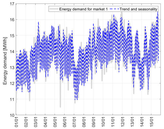
Figure 2.
Daily energy demand for Market 1 in the 2016–2018 period.
To analyse the energy demand, historical energy demand data of five (5) energy commercialization markets in Colombia in the cities of Barranquilla, Cartagena, Monteria and Santa Marta were used in the period between 1 January 2016 to 4 June 2018. Energy demand data were normalized during the building process of the forecasting models for each commercialization market. Market 1 corresponds to Barranquilla, Market 2 is Cartagena, Markets 3 and 5 belong to Monteria, while Market 4 is devoted to Santa Marta. Weather data were acquired through the website www.accuweather.com. Figure 3, Figure 4, Figure 5, Figure 6 and Figure 7 show the energy demand for Markets 1 to 5, respectively. The Dickey–Fuller test applied to the time series shows that all the considered time series had nonstationary characteristics since the null hypothesis (i.e., the existence of a unit root) was not rejected. Due to the similar characteristics of the five (5) markets, the authors decided to use Market 1 to show the proposed methodology in detail.
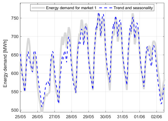
Figure 3.
Daily energy demand for Market 1 between 25 May 2018–2 June 2018.
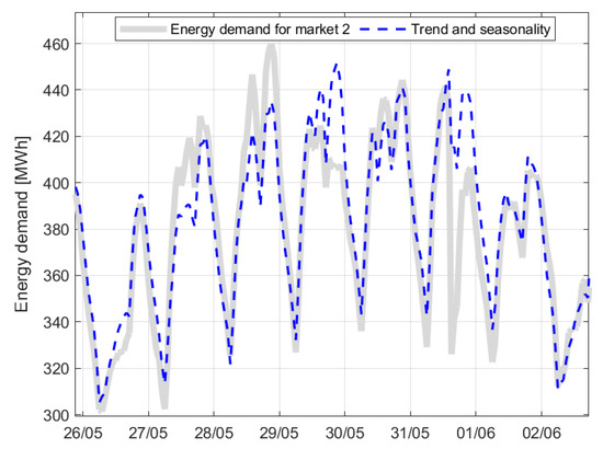
Figure 4.
Daily energy demand for Market 2 in the period between 26 May 2018–2 June 2018.
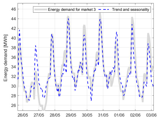
Figure 5.
Daily energy demand for Market 3 between 26 May 2018–2 June 2018.
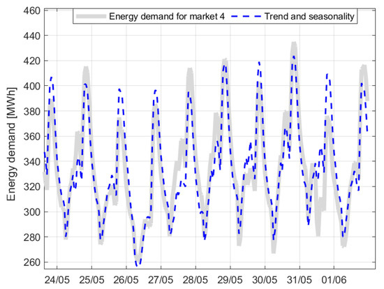
Figure 6.
Daily energy demand for Market 4 between 24 May 2018–1 June 2018.
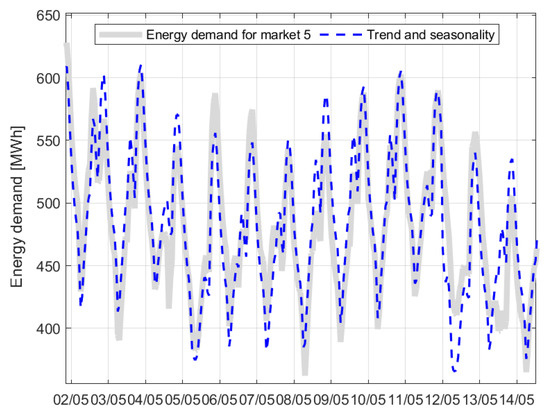
Figure 7.
Daily energy demand for Market 5 between 2–14 May 2018.
Table 1 shows the statistical characteristics of the energy demand profile. Weekdays presented similar mean and median in the energy demand, on the contrary to Saturdays and Sundays/holidays. Table 1 reveals that there was data concentration to the left of the mean due to the reported positive asymmetry. Similarly, kurtosis values were similar for all types of days and lower than three, showing a shape not as sharp and with wider tails compared to a normal distribution.

Table 1.
Summary for the statistics of the daily energy demand series.
Figure 8 shows an example of when the energy demand presents a seasonal component. This component exists due to the difference in the energy demand for Saturdays and Sundays/holidays, where there was a reduction in the consumption because several activities were stopped.
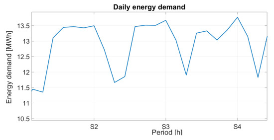
Figure 8.
Stationary for the daily energy demand series between 5 January 2018 and 8 February 2018.
On the other hand, Figure 9 shows the energy demand distribution for all types of days for each considered period. This figure represents the summary characteristics of Table 1. The energy demand data distribution for each type of day was mostly concentrated toward the left of the mean, while the variance was approximately equal for every case. A multicomparison was used to verify the existence of statistical differences in the mean of the energy demand for each type of day. Figure 10 confirms the results of Figure 8 and Figure 9.
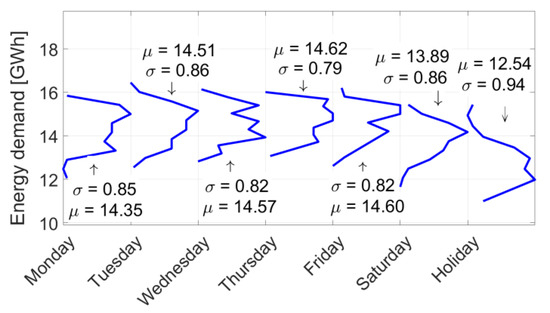
Figure 9.
Energy demand distribution for each type of day between 2016 and 2018.
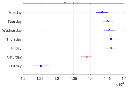
Figure 10.
Multicomparison of the daily means of the energy demand for each type of day.
So far, the obtained results in the first stage show the differences among the energy demand for weekdays, Saturdays, and Sundays/holidays. Additionally, Figure 4 shows the necessity to build a model for each day, because the shape of energy demand distribution for weekdays was different. Therefore, eight neural networks were trained using the energy demand for each day. It is important to note that a variation in the energy demand existed for a particular day within a considered period, which suggests a changing energy demand for certain times of the year. Thus, the methodology proposed the addition of a classification stage that allowed for the consideration of historical trends to determine which of them had the highest similarity.
Figure 11 shows the power spectral density (PSD) for energy demand. The spectral peaks in the frequency for the days with a high grade of information, the presence of trends and stationarity in the energy demand and the presence of a high correlation can be observed. Using the PSD and the correlation function, it is possible to observe the existence of a predominant component in the temporal series of seven days.
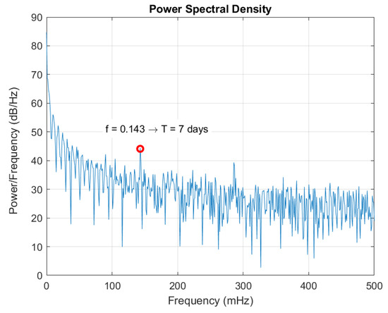
Figure 11.
Power spectral density for the daily energy demand between 2016–2018.
The autocorrelation function in Figure 12 shows a high correlation between each of the previous energy demand data and the seasonal nature of that demand. The importance of historical data for the generalization of a stationary process behaviour is clear.
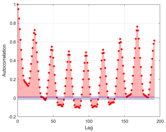
Figure 12.
Total autocorrelation for the energy demand.
Table 2 shows the correlation matrix for the energy demand and the meteorological variables for City 1, which corresponds to Market 1. This table highlights variables with a high level of correlation and data that have information about the thermal sensation of the zone of interest. Thus, humidity and wind speed were used as indicators for the thermal sensation of the considered area.
Table 2.
Energy demand correlation matrix vs. meteorological data–Market 1.
Using the results of Table 2, it can be noticed that the energy demand (D) and the temperature average (T) in the city had a high level of correlation. Therefore, the temperature was used as an external variable for the model. Similarly, as commented, the minimum humidity (H) and the maximum wind speed (W) were used to quantify the thermal sensation in the city.
As a conclusion of this procedure, a generalized methodology for the determination and selection of the input variables was proposed as:
- Tuckey-Kramer test and time-series distribution combination to identify the number of forecasting models.
- PSD analysis to assess the seasonality component of time series to add this information in the building of the base curve.
- ACF analysis to identify how many lags are necessary to build the base curve.
- Correlation matrix between weather data and energy demand to identify how the weather conditions affect the power consumption of customers.
2.2. Identification for Typical Curves in the Energy Demand
The objective for the first stage was to generate an algorithm that considered a set of curves associated with the same day of a week, clustered those curves that represented the typical behaviour of that day and rejected the ones that display different or atypical behaviour. To identify the typical curves, their normalized shapes were analysed.
For the implementation of this stage, the following actions are required:
- Normalizing the energy demand curves by dividing all the data per curve by the maximum individual value. In this way, the curves ranged between 0 and 1, and it was possible to focus on the curve shape.
- Obtaining the clustering by employing the hierarchical clustering technique. This method divided the data into sets, considering how similar they were.
- Measuring the similarity using DTW. This technique is considered the best metric for the comparison of time series. Due to the temporal characteristic in the curves of the energy demand, they were part of the set of problems in which this technique presented excellent results.
Figure 13 shows the obtained results for this stage. The typical curve is observed with a thick solid line.
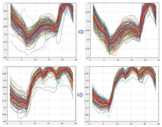
Figure 13.
Identification of typical curves for the Sunday (top row) and Monday (bottom row) for Market 1.
2.3. Generation for the Base Curves
The second stage obtains the base curve for forecasting the energy demand for each of the considered days. The goal was to generate the base curves as accurately as possible to minimize the possible corrections. Thus, the base curve was a preliminary prediction, which was obtained using statistical techniques, and it was be corrected at the final stage of the proposed methodology.
The process to obtain the base curve is described as follows:
- Once the day to be forecasted was identified, the typical curve obtained in Stage 1 was used to start the process. It is important to remember that such a curve is normalized but it represents the typical shape of the energy demand curve.
- The typical curve of that day was located at the current average level of energy demand. This was achieved by verifying the average level of the energy demand from the previous days for weekdays, and from the average level of the energy demand of the same day in the last week for Saturdays, Sundays, and holidays.
- The obtained curve was adjusted using the last four curves for the same day, obtaining the base curve.
Figure 14 shows a sample for the construction of one of the base curves for a weekday of Market 1.
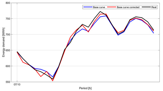
Figure 14.
Sample for a base curve of Market 1.
2.4. Intelligent Correction for the Base Curve
Stage 2 corresponds to a statistical model that allows obtaining preliminary forecasting curves (i.e., base curve), which represent mostly the expected forecast. However, they have to be slightly corrected for performance improvement. The difference between a base curve and a real one was due to the effects of external variables (i.e., temperature, humidity, and wind speed). Thus, Stage 3 employed computational intelligence techniques to adjust the forecasting base curve in the function of such external variables.
The required steps for this stage were as follows:
- The ANN technique was the computational intelligence technique used for adjusting. In total, eight independent models were obtained for each day. Each neural network had to adjust only one type of day (i.e., Sundays to Saturdays, taking the holidays as independent days).
- The input for the ANN was a function of the external variables, while the output was the adjustment that must be applied to each period (increase or reduction) to obtain a better forecasting energy demand.
- The neural networks were trained with the historical register of the last two years.
Each of the phases considered within the intelligent correction of the base of the curve is detailed below.
2.4.1. Smoothing of the Corrected Curves
In the output of Stage 3, it was possible to observe a small ripple in the forecasting energy demand curves due to the fact that a certain level of randomness exists in ANN-based models. Therefore, a smoothing technique was implemented to further enhance the performance of the proposed model.
An inverse clustering technique was implemented to smooth the curves. This process considered the four most similar curves to the obtained curve after the intelligent correction. Such curves became a reference to adjust the trace of the corrected curve and reduce the ripple to obtain the required smoothing (see Figure 15).
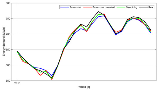
Figure 15.
Smooth of the corrected base curve obtained previously for the Sunday in Market 1.
2.4.2. Extreme Value Suppressors
Since no model is totally perfect, it was possible to obtain extreme values of the energy demand in each period of the generated curves. To correct these atypical values, if they appeared, an extreme value suppressor was applied. The suppressor allowed for better robustness, as well as an increase in reliability.
The extreme value suppressor was based on an absolute median deviation elimination using a sliding window (see Figure 16).
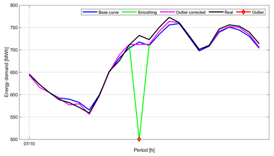
Figure 16.
Implementation of the extreme value suppressor for an ordinary day of the Market 1.
2.5. Estimation of the ANN Parameters
The neural networks training to each market was carried out iteratively, varying the number of neurons in the hidden layer. The MAPE was used as a performance metric to evaluate the level of generalization in the neural networks. The training data were energy demand data and weather data of the markets during the period 2016–2017. The year 2018 was used to verify the performance of the selected models. In general, a MultiLayer Perceptron (MLP) with sigmoid and linear activation functions in the hidden and output layers were implemented, respectively. For all markets, eight neural networks were used for each type of day, including the holidays as a special case.
In this work, the methodology for the neural networks used by the authors of [18,19,20] was considered as a reference to select the best possible configuration.
3. Results and Conclusions
The proposed methodology established a set of steps to model the behaviour of energy demand. First, energy demand data for Market 1 were used to validate the proposed methodology. This section presents the obtained results for Markets 1 to 5. The MAPE has frequently been used in the literature to measure the level of adjustment and generalization of the prediction models. It is expressed as
: Real energy demand in the period i.
: Forecasting energy demand in the period i.
N: Total data number.
Figure 17, Figure 18, Figure 19, Figure 20 and Figure 21 show the obtained results to demonstrate the proposed methodology flexibility. Table 3 shows the error percentage obtained during each adjustment stages proposed in this methodology. The results in Table 3 shows the level of contribution in the error reduction for each adjustment stage.
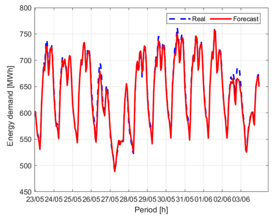
Figure 17.
Forecasting energy demand for Market 1.
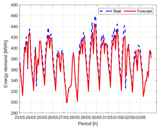
Figure 18.
Forecasting energy demand for Market 2.
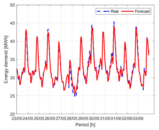
Figure 19.
Forecasting energy demand for Market 3.
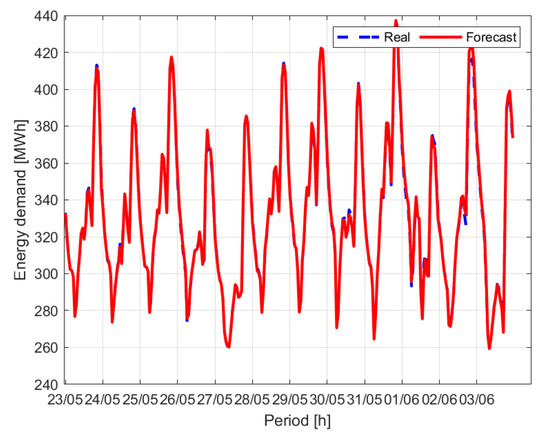
Figure 20.
Forecasting energy demand for Market 4.
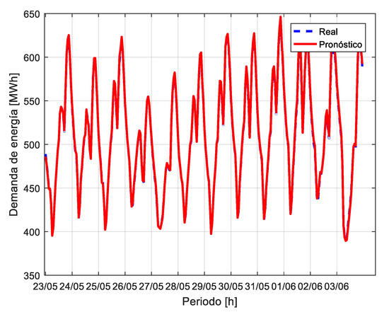
Figure 21.
Forecasting energy demand for Market 5.
Table 3.
Performance for the different stages of the methodology for the forecasting energy demand.
Table 4 shows the final performance for the obtained models for each market.
Table 4.
Performance of the models in the forecasting energy demand.
The results of Figure 17, Figure 18, Figure 19, Figure 20 and Figure 21 and Table 4 demonstrate the fulfilment of the proposed objective, since it was possible to achieve a MAPE below 5% for a 10-day forecast for each of the markets. The results show a better performance in comparison with the same demand curves described by the authors of [20].
The construction of consumption profiles proved to be a good step toward predicting demand. However, a preliminary base curve does not incorporate the effect of external variables such as weather conditions. Therefore, an intelligent correction with neural networks is necessary. Such correction technique can adjust each period independently. However, it is possible to induce ripple in the output curve. Therefore, the intelligent correction agent was complemented with mechanisms of smoothing and outliers suppressing to guarantee the best performance.
The design of an adaptive methodology capable of anticipating changes in the behavioural dynamics of the time series is proposed for future work. This will allow the automatic adjustment of the parameters of the models without affecting performance significantly. The addition of an intelligent system will help to identify when the model should be retrained or replaced by another that is available in the knowledge base that the proposed system can access to model a time series.
Author Contributions
Conceptualization, J.J.M. and C.G.Q.M.; methodology, J.J.M. and C.G.Q.M.; software, J.J.M.; validation, J.J.M.; formal analysis, J.J.M., L.N., C.G.Q.M., and M.P.; investigation, J.J.M., L.N., C.G.Q.M., and M.P.; resources, J.J.M.; data curation, J.J.M.; writing—original draft preparation, J.J.M., L.N., C.G.Q.M., and M.P.; writing—review and editing, J.J.M., L.N., C.G.Q.M., and M.P.; visualization, J.J.M.; supervision, M.P.; project administration, C.G.Q.M.; funding acquisition, J.J.M. and C.G.Q.M. All authors have read and agreed to the published version of the manuscript.
Funding
This research was supported by the Colombian Ministry of Science and Technology, MINCIENCIAS. Educational founding for national doctorates, Call No. 785.
Acknowledgments
This work was supported by Universidad del Norte, Barranquilla-Colombia.
Conflicts of Interest
The authors declare no conflict of interest.
References
- Goulermas, Q.H.; Wu, J.Y. Forecasting electric daily peak load based on local prediction. In Proceedings of the 2009 IEEE Power & Energy Society General Meeting, Calgary, AB, Canada, 26–30 July 2009; pp. 1–6. [Google Scholar] [CrossRef]
- Dalvand, M.M.; Bahram, S.; Azami, Z.; Tarimoradi, H. Long-Term Load Forecasting of Iranian Power Grid Using Fuzzy and Artificial Neural Networks. In Proceedings of the 2008 43rd International Universities Power Engineering Conference, Padova, Italy, 1–4 September 2008. [Google Scholar]
- Beccali, M.; Cellura, M.; Brano, V.L.; Marvuglia, A. Forecasting daily urban electric load profiles using artificial neural networks. Energy Convers. Manag. 2004, 45, 2879–2900. [Google Scholar] [CrossRef]
- Guo, J.W.Z.; Zhao, W.; Lu, H. Multi-step forecasting for wind speed using a modified EMD-based artificial neural network model. Renew. Energy 2012, 37, 241–249. [Google Scholar] [CrossRef]
- Dai, M.; Yu, Z.; Zeng, R. A Neural Network Short-Term Load Forecasting Considering Human Comfort Index and its Accumulative Effect. In Proceedings of the 2013 Ninth International Conference on Natural Computation (ICNC), Shenyang, China, 23–25 July 2013; pp. 262–266. [Google Scholar]
- De Andrade, L.C.M.; Da Silva, I.N. Very Short-Term Load Forecasting Based on ARIMA Model and Intelligent Systems. In Proceedings of the 2009 15th International Conference on Intelligent System Applications to Power Systems, Curitiba, Brazil, 8–12 November 2009; pp. 1–6. [Google Scholar] [CrossRef]
- García, C. Estimation and Selection of ARIMA Models. 2012. Available online: http://www.est.uc3m.es/amalonso/esp/TSAtema9petten.pdf (accessed on 3 July 2020).
- Amin, A.; Grunske, L.; Colman, A. An approach to software reliability prediction based on time series modeling. J. Syst. Softw. 2013, 86, 1923–1932. [Google Scholar] [CrossRef]
- Pai, P.; Hong, W. Forecasting regional electricity load based on recurrent support vector machines with genetic algorithms. Electr. Power Syst. Res. 2005, 74, 417–425. [Google Scholar] [CrossRef]
- Fan, S.; Chen, L. Short-Term Load Forecasting Based on an Adaptive Hybrid Method. IEEE Trans. Power Syst. 2006, 21, 392–401. [Google Scholar] [CrossRef]
- Song, K.; Baek, Y.; Hong, D.H.; Jang, G. Short-Term Load Forecasting for the Holidays Using. IEEE Trans. Power Syst. 2005, 20, 96–101. [Google Scholar] [CrossRef]
- Song, K.-B.; Ha, S.-K.; Park, J.-W.; Kweon, D.-J.; Kim, K.-H. Hybrid Load Forecasting Method with Analysis of Temperature Sensitivities. IEEE Trans. Power Syst. 2006, 21, 869–876. [Google Scholar] [CrossRef]
- Rastad, M.; Nazarzadeh, J. A Hybrid Nonlinear Model for the Annual Maximum Simultaneous Electric Power Demand. IEEE Trans. Power Syst. 2006, 21, 1069–1078. [Google Scholar]
- Wang, X.; Meng, M. Forecasting Electricity Demand Grey-Markov Model. In Proceedings of the 2008 International Conference on Machine Learning and Cybernetics, Kunming, China, 12–15 July 2008; pp. 12–15. [Google Scholar]
- Yalcinoz, T.; Eminoglu, U. Short term and medium term power distribution load forecasting by neural networks. Energy Convers. Manag. 2005, 46, 1393–1405. [Google Scholar] [CrossRef]
- Liu, D.; Zeng, L.; Li, C.; Ma, K.; Chen, Y.; Cao, Y. A Distributed Short-Term Load Forecasting Method Based on Local Weather Information. IEEE Syst. J. 2018, 12, 208–215. [Google Scholar] [CrossRef]
- Fay, D.; Ringwood, J.V. On the influence of weather forecast errors in short-term load forecasting models. IEEE Trans. Power Syst. 2010, 25, 1751–1758. [Google Scholar] [CrossRef]
- Jimenez, J.; Pertuz, A.; Quintero, C.; Montana, J. Multivariate statistical analysis based methodology for long-term demand forecasting. IEEE Lat. Am. Trans. 2019, 17, 93–101. [Google Scholar] [CrossRef]
- Wang, Y.; Chen, Q.; Sun, M.; Kang, C.; Xia, Q. An Ensemble Forecasting Method for the Aggregated Load with Subprofiles. IEEE Trans. Smart Grid 2018, 9, 3906–3908. [Google Scholar] [CrossRef]
- Jiménez, J.; Donado, K.; Quintero, C.G. A Methodology for Short-Term Load Forecasting. IEEE Lat. Am. Trans. 2017, 15, 400–407. [Google Scholar] [CrossRef]
- Gómez, M. Modelo de Previsión de Demanda de Electricidad de Largo Plazo; Universidad Pontificia Comillas: Madrid, Spain, 2010. [Google Scholar]


© 2020 by the authors. Licensee MDPI, Basel, Switzerland. This article is an open access article distributed under the terms and conditions of the Creative Commons Attribution (CC BY) license (http://creativecommons.org/licenses/by/4.0/).