2.2. Definition and Formulation of a Mixed User Equilibrium
In this paper, it is assumed that there are two kinds of vehicle drivers in the network, i.e., BEV drivers and gasoline vehicle drivers. For BEV drivers, they many need rechange their BEVs at one en-route charging station to avoid running out of charge before reaching their destinations. It is worth mentioning that this paper assumes that in order to reach the destination as quickly as possible, the BEVs will not be fully charged at the en-route charging station; BEV drivers will recharge a small amount of electricity (this also suggests that the values of travel time are higher for these BEV drivers). In addition, due to the uncertainty of fuel consumption, BEV drivers may avoid using all of the power supplied by their batteries when they arrive at the destinations. Instead, they prefer to set a battery safety margin that they keep the remaining battery higher than [
10]. Thus, we assumed that when BEV drivers arrive their destinations, the remaining battery is no less than the battery safety margin. This battery safety margin will ensure that they can find the next charging station to keep the BEV going. Note that in this paper, the minimal recharging amount of electricity depends on the remaining distance traveled and BEV drivers’ battery safety margins.
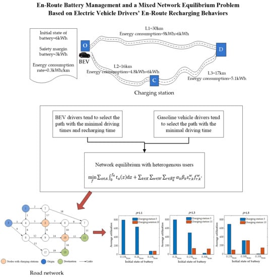
Figure 1 is an example used to illustrate the en-route recharging behavior. As shown in
Figure 1, the BEV’s initial state of battery is 6 kWh, the energy consumption rate is 0.3 kWh/km [
18], and the BEV driver’s battery safety margin is 3 kWh. Then, under this setting, this BEV driver will choose path 2 and the amount of recharging electricity will be 6.9 kWh. On the other hand, for gasoline vehicle drivers, it is assumed that they have enough fuel.
When traveling between their original location and destination, for each driver, it is assumed that they select the route with minimal travel costs, which includes the cost of travel time and electricity. It is worth mentioning that the cost of travel time is much higher than the cost of electricity [
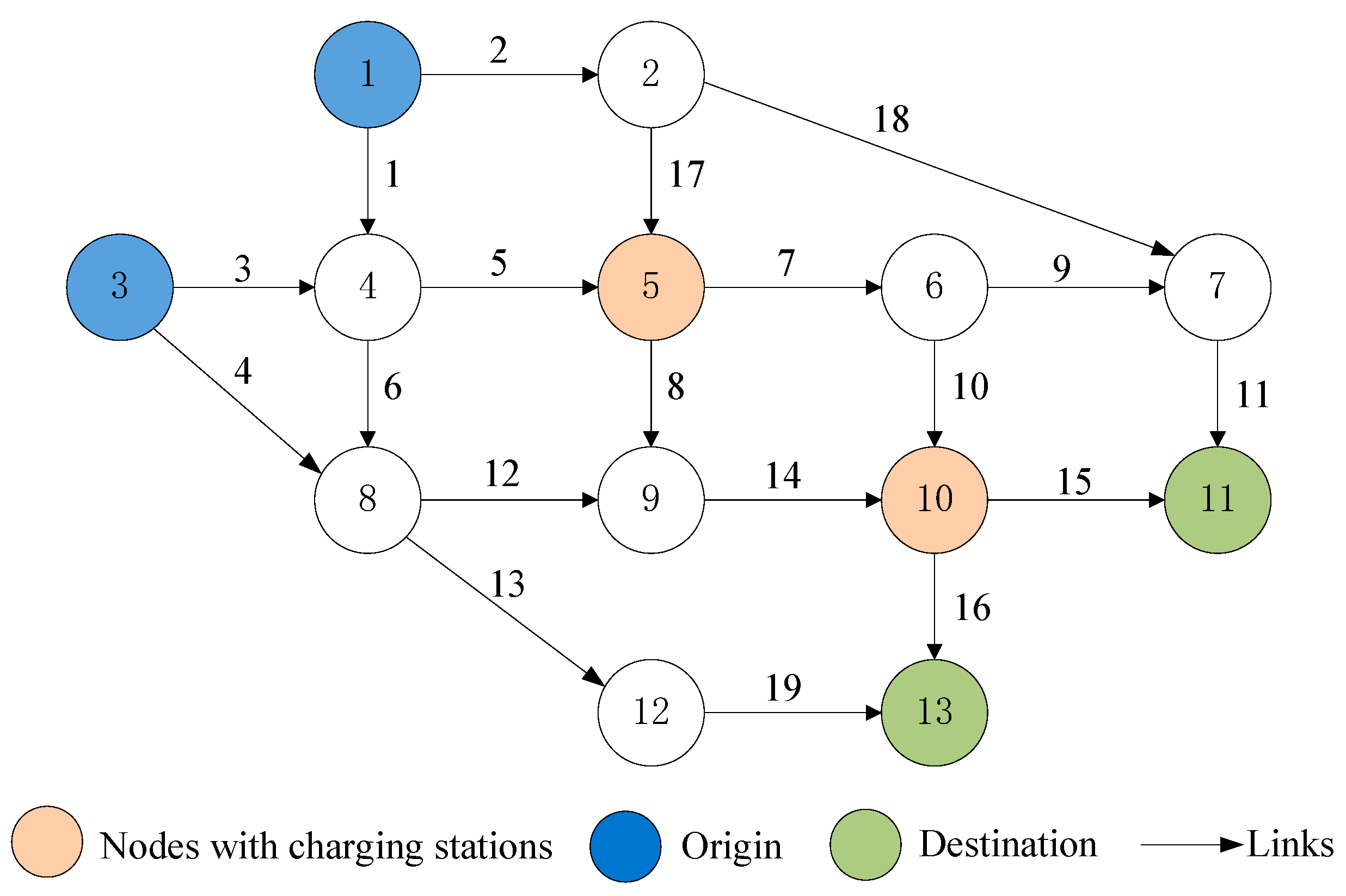
25]. Thus, we only consider travel time cost when drivers select paths. Notably, for BEV drivers who need recharging en-route, their total travel time includes driving time and recharging time. Moreover, different from others’ research, in our based model, we consider heterogenous BEV drivers with different risk attitudes and different levels of perception errors regarding the values of recharging time, and the BEVs have the same battery size but a different initial state of battery. Moreover, we further assumed that in the transport network, there is only a finite number of charging stations, and these charging stations are located at certain nodes of the network. Note that a vehicle traveling along a path may not pass by a charging station. Thus, based on the above assumptions and considerations, we can obtain the following network equilibrium:
Definition 1. In a long-term equilibrium, for the same type of drivers, all the utilized paths are usable and the total travel time costs of all the utilized paths of one OD pair are the same, that is, they are less than or equal to those of any unutilized usable paths of the same OD pair.
Here, a mathematic model will be proposed to describe the above long-term equilibrium. For convenience, it is assumed that there are
types of vehicle drivers in the network where
types belong to BEV drivers and they have different risk attitudes and different levels of perception of rechanging time. The remaining type belongs to gasoline vehicle drivers. Moreover, because BEV energy consumption is independent of traffic flow, let
denote the set of all usable paths between OD pair
, thus, we can obtain following network equilibrium with heterogenous users (NE-HU):
where,
is the minimal actual time (minutes) that drivers need to spend on recharging activity. Moreover, for gasoline vehicle drivers, there is
= 0.
is a coefficient and relates to the drivers’ risk attitudes.
is a coefficient and relates to BEV drivers’ perception errors of the values of recharging time. Note that limited by cognitive ability, drivers may not be able to accurately estimate their recharging times, thus, the “perception error” in this study is defined as the difference between a BEV driver’s perceived value of recharging time and the actual value of recharging time. Moreover,
= 1 indicates that a driver’s perception of disutility of unit travel time is equal to their perception of disutility of unit recharging time, and the greater the value of
, the smaller the perception of disutility of unit recharging time.
is travel demand (i.e., total vehicles) of type
between OD pair
, and
(veh/h) is the traffic flow of type
on path
between OD pair
.
Then, the above NE-HU model’s Karush-Kuhn-Tucker (KKT) conditions can be written as:
where
and
. Moreover,
is the travel time (minutes) of path
. Thus, Equation (7) can be further written as:
Finally, based on the Equations (10)–(12), we can obtain the following conditions:
Here, Equation (14) is a complementary condition. When
, if
, then
; if
, then
. However, when
,
. This complementary condition guarantees that the traffic flow is only distributed on the usable paths.
2.3. Solution Procedure
The above NE-HU model is a convex program with linear constraints. We can solve it by the enumeration method. However, the work of enumerating all the usable paths will be tremendous. Thus, in this paper, we adopt an iterative solution procedure which was proposed by He et al. [
18]. However, different from He’s work, in this paper, we consider the perception recharging time instead of actual recharging time and heterogenous BEV drivers with the different risk attitudes and different levels of perception of recharging time. Thus, the sub-problem, finding the shortest usable path by considering BEV drivers’ perception of recharging time (SP-PT), can be formulated as follows:
where,
(kWh) is the recharging amount of electricity in theory at charging stations
for type
drivers, and
(kWh) is the actual recharging amount of electricity for type
drivers when considering their different risk attitudes. Let
represent the recharging time (minutes) that at node
, type
drivers spend recharging
amount of electricity. Then,
is the perception of time for type
drivers to recharge
amount of electricity. In this paper, the following perception of charging time function is used, i.e.,
, and here
(minutes) represents the fixed recharging time;
(
) is a variable of recharging time and relies on the class of chargers, for example, direct current charging (fast charging) and alternating current charging (slow charging). However, in this study, it is assumed that the en-route charging stations only supply direct current charging facilities and the charging facilities are adequate. Note that if there is no charging station on node
, the value of
will be zero, and for gasoline vehicle drivers, the value of
will also be zero.
Moreover, (kWh) is the battery charge after recharging, (kWh) is the battery size, and (kWh) is the initial state of battery charge. is the node-link incidence matrix, is a vector with a length of and consists of two nonzero components: one has a value of 1, which corresponds to the original location; the other has a value of −1 which corresponds to the destination. is a binary variable, and if link is used, then , otherwise ; is also a binary variable, and if charging station is selected, then , otherwise, . if link is used by driver and unrestriced otherwise. is the BEV’s energy consumption, is the minimum comfortable range, and and are sufficiently large constants.
In the above SP-PT model, the objective function is to minimize the total trip time, including driving time (i.e., ) and BEV drivers’ perceived recharging time (i.e., . Constraint (16) ensures flow balance. Constraints (17) and (19) specify the relationship between the states of charge of BEV batteries at the starting and ending nodes of any utilized link. Constraint (18) ensures that the BEV driver will not fully deplete their battery on any utilized link, and the BEV driver prefers to keep the remaining battery range no less than a comfortable range.
Let be the optimal solution to SP-PT for OD pair for each type of . By solving , we can obtain the shortest usable path, i.e., . Moreover, through solving and , we can obtain the shortest perception recharging time, i.e., . Then, to solve NE-HU, we can use the following iterative procedures:
Step 1: For each type of between OD pair solve SP-PT, i.e., . Obtain the initial usable path set and calculate the minimal actual recharging time .
Step 2: Based on the initial usable path set , solve the NE-HU model and obtain the optimal traffic flow distribution, i.e., and the Lagrange multiplier, i.e., .
Step 3: Solve the SP-PT model. For each type of and each OD pair , if , then stop and is the optimal equilibrium link flow distribution; otherwise, go to Step 1.


