Scoring Model of the Financial Health of the Electrical Engineering Industry’s Non-Financial Corporations


Abstract
:
1. Introduction
2. Literature Review
2.1. New Era in Forecasting Financial Developments in Enterprises
2.1.1. Multiple Discriminant Analysis
2.1.2. Logit Analysis and Neural Networks
2.2. Financial Health of Non-Financial Corporations from the Electrical Engineering Industry
3. Materials and Methods
3.1. Research Sample
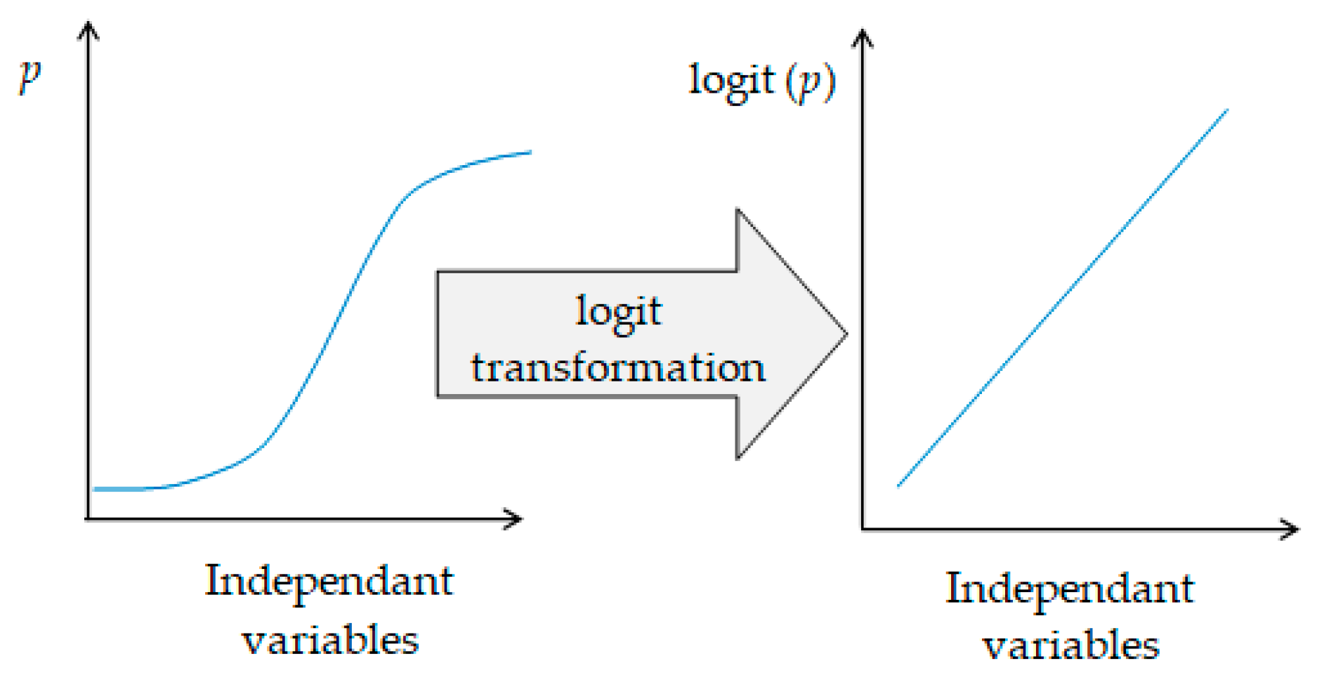
3.2. Logistic Regression
- For any combination of possible values ß0, ß1, …, ßn, the probability function tells us how likely we are to observe the data we observed if the model of the estimated parameter values were real parameters in the population.
- If we imagine a surface in which the range of possible values β0 represents one axis and the range of β is the second axis, the resulting probability function graph would look like a hill, where ML estimates would be the values of the parameters corresponding to the peak of that hill. The variance of possible estimates corresponds roughly to how quickly the slope changes, in a place near the top.
- MML is the common probability density of all observed responses Yij as a function of model parameters β0, β, σ2.
- The principle is to find an estimate of the parameters β0, β, σ2, that maximize this probability function, leading to a solution that appears to be probable as much as possible (maximum likelihood).
- MLs have good properties: They are consistent (as the size of the sample increases, the estimates approximate to the actual value); they are efficient (they have the smallest possible variance in large selections); and asymptotic normal (approaching normal distribution).
4. Results
5. Discussion and Conclusions
Author Contributions
Funding
Acknowledgments
Conflicts of Interest
Appendix A

| PL | Correct | Incorrect | Percentages | ||||||
|---|---|---|---|---|---|---|---|---|---|
| E | NE | E | NE | Correct | Sensitivity | Specificity | False POS | False NEG | |
| 0.000 | 111 | 0 | 739 | 0 | 13.1 | 100.0 | 0.0 | 86.9 | . |
| 0.020 | 108 | 338 | 401 | 3 | 52.5 | 97.3 | 45.7 | 78.8 | 0.9 |
| 0.040 | 107 | 414 | 325 | 4 | 61.3 | 96.4 | 56.0 | 75.2 | 1.0 |
| 0.060 | 107 | 473 | 266 | 4 | 68.2 | 96.4 | 64.0 | 71.3 | 0.8 |
| 0.080 | 107 | 523 | 216 | 4 | 74.1 | 96.4 | 70.8 | 66.9 | 0.8 |
| 0.100 | 106 | 573 | 166 | 5 | 79.9 | 95.5 | 77.5 | 61.0 | 0.9 |
| 0.120 | 104 | 617 | 122 | 7 | 84.8 | 93.7 | 83.5 | 54.0 | 1.1 |
| 0.140 | 101 | 655 | 84 | 10 | 88.9 | 91.0 | 88.6 | 45.4 | 1.5 |
| 0.160 | 97 | 675 | 64 | 14 | 90.8 | 87.4 | 91.3 | 39.8 | 2.0 |
| 0.180 | 90 | 690 | 49 | 21 | 91.8 | 81.1 | 93.4 | 35.3 | 3.0 |
| 0.200 | 85 | 702 | 37 | 26 | 92.6 | 76.6 | 95.0 | 30.3 | 3.6 |
| 0.220 | 82 | 708 | 31 | 29 | 92.9 | 73.9 | 95.8 | 27.4 | 3.9 |
| 0.240 | 80 | 717 | 22 | 31 | 93.8 | 72.1 | 97.0 | 21.6 | 4.1 |
| 0.260 | 78 | 719 | 20 | 33 | 93.8 | 70.3 | 97.3 | 20.4 | 4.4 |
| 0.280 | 78 | 722 | 17 | 33 | 94.1 | 70.3 | 97.7 | 17.9 | 4.4 |
| 0.300 | 77 | 725 | 14 | 34 | 94.4 | 69.4 | 98.1 | 15.4 | 4.5 |
| 0.320 | 75 | 728 | 11 | 36 | 94.5 | 67.6 | 98.5 | 12.8 | 4.7 |
| 0.340 | 73 | 729 | 10 | 38 | 94.4 | 65.8 | 98.6 | 12.0 | 5.0 |
| 0.360 | 71 | 729 | 10 | 40 | 94.1 | 64.0 | 98.6 | 12.3 | 5.2 |
| 0.380 | 71 | 732 | 7 | 40 | 94.5 | 64.0 | 99.1 | 9.0 | 5.2 |
| 0.400 | 70 | 733 | 6 | 41 | 94.5 | 63.1 | 99.2 | 7.9 | 5.3 |
| 0.420 | 70 | 733 | 6 | 41 | 94.5 | 63.1 | 99.2 | 7.9 | 5.3 |
| 0.440 | 70 | 733 | 6 | 41 | 94.5 | 63.1 | 99.2 | 7.9 | 5.3 |
| 0.460 | 69 | 733 | 6 | 42 | 94.4 | 62.2 | 99.2 | 8.0 | 5.4 |
| 0.480 | 67 | 733 | 6 | 44 | 94.1 | 60.4 | 99.2 | 8.2 | 5.7 |
| 0.500 | 64 | 733 | 6 | 47 | 93.8 | 57.7 | 99.2 | 8.6 | 6.0 |
| 0.520 | 62 | 734 | 5 | 49 | 93.6 | 55.9 | 99.3 | 7.5 | 6.3 |
| 0.540 | 59 | 734 | 5 | 52 | 93.3 | 53.2 | 99.3 | 7.8 | 6.6 |
| 0.560 | 57 | 734 | 5 | 54 | 93.1 | 51.4 | 99.3 | 8.1 | 6.9 |
| 0.580 | 56 | 734 | 5 | 55 | 92.9 | 50.5 | 99.3 | 8.2 | 7.0 |
| 0.600 | 55 | 734 | 5 | 56 | 92.8 | 49.5 | 99.3 | 8.3 | 7.1 |
| 0.620 | 54 | 734 | 5 | 57 | 92.7 | 48.6 | 99.3 | 8.5 | 7.2 |
| 0.640 | 54 | 734 | 5 | 57 | 92.7 | 48.6 | 99.3 | 8.5 | 7.2 |
| 0.660 | 53 | 734 | 5 | 58 | 92.6 | 47.7 | 99.3 | 8.6 | 7.3 |
| 0.680 | 52 | 734 | 5 | 59 | 92.5 | 46.8 | 99.3 | 8.8 | 7.4 |
| 0.700 | 51 | 734 | 5 | 60 | 92.4 | 45.9 | 99.3 | 8.9 | 7.6 |
| 0.720 | 49 | 734 | 5 | 62 | 92.1 | 44.1 | 99.3 | 9.3 | 7.8 |
| 0.740 | 48 | 734 | 5 | 63 | 92.0 | 43.2 | 99.3 | 9.4 | 7.9 |
| 0.760 | 46 | 734 | 5 | 65 | 91.8 | 41.4 | 99.3 | 9.8 | 8.1 |
| 0.780 | 43 | 734 | 5 | 68 | 91.4 | 38.7 | 99.3 | 10.4 | 8.5 |
| 0.800 | 39 | 734 | 5 | 72 | 90.9 | 35.1 | 99.3 | 11.4 | 8.9 |
| 0.820 | 39 | 734 | 5 | 72 | 90.9 | 35.1 | 99.3 | 11.4 | 8.9 |
| 0.840 | 36 | 734 | 5 | 75 | 90.6 | 32.4 | 99.3 | 12.2 | 9.3 |
| 0.860 | 33 | 734 | 5 | 78 | 90.2 | 29.7 | 99.3 | 13.2 | 9.6 |
| 0.880 | 32 | 734 | 5 | 79 | 90.1 | 28.8 | 99.3 | 13.5 | 9.7 |
| 0.900 | 31 | 734 | 5 | 80 | 90.0 | 27.9 | 99.3 | 13.9 | 9.8 |
| 0.920 | 30 | 734 | 5 | 81 | 89.9 | 27.0 | 99.3 | 14.3 | 9.9 |
| 0.940 | 30 | 735 | 4 | 81 | 90.0 | 27.0 | 99.5 | 11.8 | 9.9 |
| 0.960 | 26 | 735 | 4 | 85 | 89.5 | 23.4 | 99.5 | 13.3 | 10.4 |
| 0.980 | 22 | 736 | 3 | 89 | 89.2 | 19.8 | 99.6 | 12.0 | 10.8 |
| 1.000 | 0 | 739 | 0 | 111 | 86.9 | 0.0 | 100.0 | . | 13.1 |
References
- Statistical Office of the Slovak Republic. DATAcube. Available online: http://datacube.statistics.sk/ (accessed on 31 July 2020).
- Mládek, J. Teritoriálne Priemyselné Útvary Slovenska; Univerzita Komenského: Bratislava, Slovakia, 1990. [Google Scholar]
- Dubcová, A.; Midler, M. Impact of foreign capital on disparities of electrical engineering industry in districts of Slovakia. Geogr. Inf. 2014, 18, 49–58. [Google Scholar] [CrossRef]
- Kulla, M. Súčasný stav a vývojové trendy v elektrotechnickom priemysle Slovenska. Acta Geogr. Univ. Comen. 2013, 57, 31–49. [Google Scholar]
- Mišunová, E.; Mišun, J. Priemysel Slovenska a Dopady Globálnej Krízy. Globálna Kríza s Akcentom na Automobilový Priemysel; Espirit: Bratislava, Slovak, 2009. [Google Scholar]
- Laatu, M.; Takala, J. Implementing European quality award in a global high tech company. Int. J. Technol. Manag. 1999, 17, 869–884. [Google Scholar] [CrossRef]
- Fertala, N. Growth and competition in the economic “wonder years”: The electrotechnical industry in the Federal Republic of Germany and in Great Britain, 1945–1967. Bus. Hist. 2005, 47, 311–312. [Google Scholar]
- Plumpe, W. Growth and competition in the years of the Economic Miracle. The electrotechnical industry in the Federal Republic of Germany and in Great Britain, 1945–1967. Hist. Z. 2003, 277, 264–267. [Google Scholar]
- Fischer, M.; Menschik, G. Innovations and technological-change in Austria. Mitt. Osterreichischen Geogr. Ges. 1991, 133, 43–68. [Google Scholar]
- Jenčová, S. Aplikácia Pokročilých Metód vo Finančno-Ekonomickej Analýze Elektrotechnického Odvetvia Slovenskej Republiky; SAEI VŠB-TU Ostrava: Ostrava, Czech Republic, 2018. [Google Scholar]
- Štefko, R.; Jenčová, S.; Vašaničová, P.; Litavcová, E. An Evaluation of Financial Health in the Electrical Engineering Industry. J. Compet. 2019, 11, 144–160. [Google Scholar]
- Jenčová, S.; Vašaničová, P.; Litavcová, E. Financial indicators of the company from electrical engineering industry: The case study of Tesla, Inc. Serb. J. Manag. 2019, 14, 361–371. [Google Scholar] [CrossRef]
- Jenčová, S.; Litavcová, E.; Vašaničová, P. Implementation of Du Pont model in non-financial corporations. Montenegrin J. Econ. 2018, 14, 131–141. [Google Scholar] [CrossRef]
- Jenčová, S.; Litavcová, E.; Vašaničová, P. Implementation of financial and statistical models to study the electrical industry of the Slovak republic. In Political Sciences, Law, Finance, Economics and Tourism. In Proceedings of the 3rd International Multidisciplinary Scientific Conference Social Sciences & Arts SGEM 2016, Sofia, Bulgaria, 22–31 August 2016; Sofia: STEF92 Technology: Sofia, Bulgaria, 2016; pp. 329–336. [Google Scholar]
- Kislingerová, E.; Hnilica, J. Finanční Analýza—Krok za Krokem; C.H. Beck: Prague, Czech Republic, 2005. [Google Scholar]
- Tamari, M. Financial ratios as a means of forecasting bankruptcy. Manag. Int. Rev. 1966, 4, 15–21. [Google Scholar]
- Doucha, R. Finanční Analýza Podniku; Vox Consult: Praha, Czech Republic, 1996. [Google Scholar]
- Fitzpatrick, P.J. A Comparison of ratios of successful industrial enterprises with those of failed firms. Certif. Public Account. 1932, 10, 598–605. [Google Scholar]
- Smith, R.F.; Winakor, A.H. Changes in the Financial Structure of Unsuccessful Industrial Corporations; University of Illinois: Urbana, IL, USA, 1935. [Google Scholar]
- Merwin, C.L. Financing Small Corporations in Five Manufacturing Industries, 1926–1936; National Bureau of Economic Research: New York, NY, USA, 1942. [Google Scholar]
- Chudson, W.A. A Survey of Corporate Financial Structure; National Bureau of Economic Research: New York, NY, USA, 1945. [Google Scholar]
- Walter, J. Determination of technical insolvency. J. Bus. 1957, 30–43. [Google Scholar] [CrossRef]
- Jackendoff, N. A study of published industry financial and operating ratios. Bur. Econ. Bus. Res. 1962, 52. [Google Scholar]
- Beaver, W. Financial ratios predictors of failure. Empirical research in accounting selected studies. J. Account. Res. 1966, 4, 71–111. [Google Scholar] [CrossRef]
- Delina, R.; Packová, M. Validácia predikčných bankrotových modelov v podmienkach SR. E + M. Ekonómie Manag. 2013, 16, 101–112. [Google Scholar]
- Altman, E.I. Financial ratios, discriminant analysis and the prediction of corporate bankruptcy. J. Financ. 1968, 23, 589–609. [Google Scholar] [CrossRef]
- Altman, E.I. Predicting financial distress of companies: Revisiting the Z-Score and ZETA® models. In Handbook of Research Methods and Applications in Empirical Finance Chapters; Bell, A.R., Brooks, C., Prokopczuk, M., Eds.; Edward Elgar Publishing: Cheltenham Glos, UK, 2013; Volume 1, pp. 428–456. [Google Scholar]
- Altman, E.I.; Iwanicz-Drozdowska, M.; Laitinen, E.K.; Suvas, A. Distressed firm and bankruptcy prediction in an international context: A review and empirical analysis of Altman’s Z-Score Model. SSRN Electron. J. 2014, 47. [Google Scholar] [CrossRef] [Green Version]
- Deakin, E. A discriminant analysis of predictors of business failure. J. Account. Res. 1972, 10, 167–179. [Google Scholar] [CrossRef]
- Blum, M. Failing company discriminant analysis. J. Account. Res. 1974, 12, 1–25. [Google Scholar] [CrossRef]
- Sinkey, J.F. A multivariate statistical analysis F the characteristics of problem banks. J. Financ. 1975, 20, 21–36. [Google Scholar] [CrossRef]
- Beerman, K. Possible Ways of Predict Capital Losses with Annual Financial Statements; University of Düsseldorf: Dusseldorf, Germany, 1976. [Google Scholar]
- Taffler, R.J.; Tisshaw, H. Going Gone—Four Factors which predict. Accountancy 1977, 88, 50–54. [Google Scholar]
- Taffler, R.J.; Tseung, M. Going, going, going—Four factors which predict. Account. Mag. 1984, 88, 263–269. [Google Scholar]
- Springate, G.L. Predicting the Possibility of Failure in a Canadian Firm. Ph.D. Thesis, Simon Fraser University, Burnaby, Canada, 1978. Unpublished Work. [Google Scholar]
- Sands, E.G.; Springate, G.L.; Var, T. Predicting business failures. CGA Mag. 1983, 24–27. [Google Scholar]
- Fulmer, J.G.J.; Moon, J.E.; Gavin, T.A.; Erwin, M.J. Bankruptcy classification model for small firms. J. Commer. Bank Lend. 1984, 25–37. [Google Scholar]
- Marais, D.A.J. A Method of Quantifying Companies Relative Financial Strength; Bank of England: London, UK, 1979. [Google Scholar]
- Bilderbeek, J. An empirical study of the predictive ability of financial ratios in The Netherlands. Zeitschift Betr. 1979, 5, 388–407. [Google Scholar]
- Lussier, R.N. A nonfinancial business success versus failure prediction model for young firms. J. Small Bus. Manag. 1995, 33, 8–20. [Google Scholar]
- Laitinen, E.K. Traditional versus operating cash flow in failure prediction. J. Bus. Financ. Account. 1994, 21, 215–228. [Google Scholar] [CrossRef]
- Neumaierová, I.; Neumaier, I. Proč se ujal index IN a nikoli pyramídový systém ukazatelů INFA. Ekon. Manag. 2008, 2, 12–19. [Google Scholar]
- Virag, M.; Nyitrai, T. Is There a Trade-off between the predictive power and the interpretability of bankruptcy models? The case of the first Hungarian bankruptcy prediction model. Acta Oeconomica 2014, 64, 19–440. [Google Scholar] [CrossRef]
- Gurčík, Ľ. G-index-metóda predikcie finančného stavu poľnohospodárskych podnikov. Zemědělská Ekon. 2002, 48, 373–378. [Google Scholar]
- Chrastinová, Z. Metódy Hodnotenia Ekonomickej Bonity a Predikcie Finančnej Situácie Poľnohospodárskych Podnikov; VÚEPP: Bratislava, Slovak, 1998. [Google Scholar]
- Kameníková, K. Obmedzenia použitia modelov predikcie finančného vývoja podniku v podmienkach Slovenskej republiky. Acta Montan. Slovaca 2005, 10, 337–343. [Google Scholar]
- Pilch, C. K modelom hodnotenia finančného zdravia podniku. 3. časť. Finančné Trhy 2008, 5, 1–9. [Google Scholar]
- Pilch, C. K modelom hodnotenia finančného zdravia podniku. 4. časť. Finančné Trhy 2008, 5, 1–7. [Google Scholar]
- Bondareva, I. Analysis of explanatory models of the predictive ability of the financial condition of the company in Slovakia. In Proceedings of the Manažment Podnikania a Vecí Verejných: Zborník Vedeckých Prác; SAM: Bratislava, Slovakia, 2011; pp. 59–64. [Google Scholar]
- Kadarová, J.; Turisová, R. Finančné modely predikcie finančných problémov v priemyselných podnikoch. In Modelování, Simulace a Optimalizace Podnikových Procesů v Prax, Proceedings of the Sborník z Konference, Prague, Czech Republic, 29 March 2011; Tuček, D., Ed.; ČSOP: Prague, Czech Republic, 2011; pp. 167–173. [Google Scholar]
- Malega, P.; Bjalončíkováa, M. Analýza Finančného Zdravia Spoločnosti. In Zborník Vedeckých Prác Katedry Ekonómie a Ekonomiky ANNO; Kotulič, R., Ed.; University of Prešov: Prešov, Slovakia, 2012; pp. 171–183. [Google Scholar]
- Kabát, L.; Sobeková Majková, M.; Vincúrová, Z. Hodnotenie Podniku a Analýza Jeho Finančného Zdravia; Iura Edition: Bratislava, Slovak, 2013. [Google Scholar]
- Gundová, P. Využitie metód multikriteriálneho hodnotenia a neurónových sietí vo finančnom riadení a rozhodovaní. In Proceedings of the MERKUR 2012, Ekonóm: Brartislava, Bratislava, Slovakia, 6–7 December 2012; pp. 1–16. [Google Scholar]
- Gundová, P. Verifikácia vybraných predikčných metód na vzorke Slovenských podnikov. Acta Acad. Karviniensia 2014, 17, 26–38. [Google Scholar] [CrossRef] [Green Version]
- Ohlson, J.A. Financial Ratios and the Probabilistic Prediction of Bankruptcy. J. Account. Res. 1980, 18, 109–131. [Google Scholar] [CrossRef] [Green Version]
- Zavgren, C.V. Assessing the vulnerability to failure of American industrial firms: A logistic analysis. J. Bus. Financ. Account. 1985, 12, 19–45. [Google Scholar] [CrossRef]
- Jabeur, S.B. Bankruptcy prediction using partial least squares logistic regression. J. Retail. Consum. Serv. 2017, 36, 197–202. [Google Scholar] [CrossRef]
- Wang, Y. Financial ratios and the prediction of bankruptcy: The Ohlson model applied to Chinese publicly traded companies. J. Organ. Leadersh. Bus. 2010, 5, 1–15. [Google Scholar]
- Marcinkevičius, R.; Kanapickienė, R. Bankruptcy prediction in the sector of construction in Lithuania. Procedia Soc. Behav. Sci. 2014, 156, 553–557. [Google Scholar] [CrossRef]
- Slavíček, O.; Kuběnka, M. Bankruptcy prediction models based on the logistic regression for companies in the Czech Republic. In Proceedings of the 8th International Scientific Conference Managing and Modelling of Financial Risks, Ostrava, Czech Republic, 5–6 September 2016; pp. 924–931. [Google Scholar]
- Režňáková, M.; Karas, M. Bankruptcy Prediction Models: Can the prediction power of the models be improved by using dynamic indicators? Procedia Econ. Financ. 2014, 12, 565–574. [Google Scholar] [CrossRef]
- Jakubík, P.; Teplý, P. The JT Index as indicator of financial stability of corporate sector. Prague Econ. Pap. 2011, 20, 157–176. [Google Scholar] [CrossRef]
- Gurný, P.; Gurný, M. Logit and probit model within estimation of US banks. In Proceedings of the 47th EWGFM Meeting, Ostrava, Czech Republic, 28–30 October 2010; pp. 73–80. [Google Scholar]
- Valecký, J.; Slivková, E. Mikroekonomický scoringový model úpadku českých podniků. Ekon. Rev. ER-CEREI 2012, 15, 15–26. [Google Scholar] [CrossRef] [Green Version]
- Binkert, C.H.H. Fruherkennung von Unternehmenskrisen mit Hilfe Geeigneter Methoden im Deutschen und Slowakischen Wirtschaftsraum. Ph.D. Thesis, University of Economics in Bratislava, Bratislava, Slovakia, 1999. [Google Scholar]
- Hurtosova, J. Konštrukcia Ratingového Modelu, Nástroja Hodnotenia Úverovej Spôsobilosti Podniku. Ph.D. Thesis, Economic University in Bratislava, Bratislava, Slovakia, 2009. [Google Scholar]
- Vlkolinský, P. Prehľad vývoja ratingových modelov vo vybranných krajinách. Finančný Manažér 2013, 13, 17–27. [Google Scholar]
- Kováčova, M.; Klieštik, T. Logit and Probit application for the prediction of bankruptcy in Slovak companies. Equilibrium. Q. J. Econ. Econ. Policy 2017, 12, 775–791. [Google Scholar]
- Harumová, A.; Janisová, M. Hodnotenie slovenských podnikov pomocou skóringovej funkcie. Ekon. Časopis 2014, 62, 522–539. [Google Scholar]
- Sharda, R.; Wilson, R.L. Neural network experiments in business-failure forecasting: Predictive performance measurement issues. Int. J. Comput. Intell. Organ. 1996, 1, 107–117. [Google Scholar]
- Alaka, H.A.; Oyedele, L.O.; Owolabi, H.A.; Kumar, V.; Ajayi, S.O.; Akinade, O.O.; Bilal, M. Systematic review of bankruptcy prediction models: Towards a framework for tool selection. Expert Syst. Appl. 2018, 94, 164–184. [Google Scholar] [CrossRef]
- Taffler, R.J. Forecasting companyfailure in the UK using discriminant analysis and financial ratio data. J. R. Stat. Soc. 1982, 145, 342–358. [Google Scholar]
- Tsindeliani, I.; Kot, S.; Vasilyeva, E.; Narinyan, L. Tax system of the russian federation: Current state and steps towards financial sustainability. Sustainability 2019, 11, 6994. [Google Scholar] [CrossRef] [Green Version]
- Hussain, H.I.; Kot, S.; Thaker, H.M.T.; Turner, J.J. Environmental reporting and speed of adjustment to target leverage: Evidence from a dynamic regime switching model. Organizacija 2020, 53, 21–35. [Google Scholar] [CrossRef] [Green Version]
- Zmijewski, M.E. Methodological issues related to the estimation of financial distress prediction models. J. Account. Res. 1984, 22, 59–86. [Google Scholar] [CrossRef]
- Zalai, K.; Dávid, A.; Šnircová, J.; Moravčíková, E.; Hurtošová, J.; Tučníková, D. Finančno-Ekonomická Analýza; Sprint Dva: Bratislava, Slovakia, 2016. [Google Scholar]
- Stankovičová, I.; Vojtková, M. Viacrozmerné Štatistické Metódy s Aplikáciami; Grada Publishing: Praha, Czech Republic, 2007. [Google Scholar]
- Hosmer, D.W.; Lemeshow, S. Applied Logistic Regresion; Wiley: New York, NY, USA, 1989. [Google Scholar]
- Hosmer, D.W.S.; Lemeshow, S.; Sturdivant, R.X. Applied Logistic Regression, 3rd ed.; Wiley: New York, NY, USA, 2013. [Google Scholar]
- Act No. 513/1991 Coll. Commercial Code; Iura Edition: Bratislava, Slovakia, 2013. [Google Scholar]
- Act No. 7/2005 Coll. Bankruptcy and Restructuring; Iura Edition: Bratislava, Slovakia, 2013. [Google Scholar]

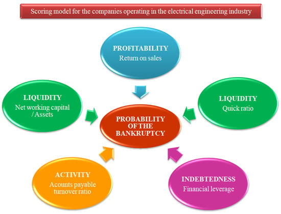
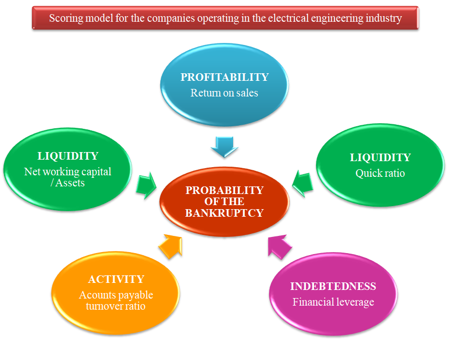
| Variable | Description |
|---|---|
| x1 | Accounts payable turnover ratio (APTR), the time during which the company pays its trade obligations |
| x2 | Return on sales (ROS) = earnings before interest, taxes, depreciation and amortization (EBITDA)/sales, |
| x3 | Return on investments (ROI) = earnings before interest, taxes (EBT)/total capital |
| x4 | quick ratio (QR) = (current assets − inventory)/current liabilities |
| x5 | sales/assets |
| x6 | Foreign capital/assets |
| x7 | Financial leverage (FL) = assets/equity |
| x8 | Net working capital (NWC)/assets (A) |
| Variables | ||||||||
|---|---|---|---|---|---|---|---|---|
| x1 | x2 | x3 | x4 | x5 | x6 | x7 | x8 | |
| 1 | 0.0013 | −0.0559 | −0.0032 | −0.0317 | 0.5875 d | −0.0037 | −0.0007 | x1 |
| 1 | 0.0034 | 0.0022 | 0.0346 | 0.0010 | 0.0048 | 0.3036 d | x2 | |
| 1 | 0.0025 | 0.0265 | −0.8403 d | 0.0034 | 0.0017 | x3 | ||
| 1 | −0.0414 | −0.0039 | −0.0067 | 0.0271 | x4 | |||
| 1 | −0.036 | −0.0209 | −0.0238 | x5 | ||||
| 1 | −0.0047 | −0.0020 | x6 | |||||
| 1 | −0.0028 | x7 | ||||||
| 1 | x8 | |||||||
| Variable | B | S.E. | Wald Chi-Square | OR | LCI | UCI |
|---|---|---|---|---|---|---|
| Intercept | −1.4988 d | 0.2687 | 31.1176 | |||
| x1 − APTR | 0.0218 d | 0.0083 | 6.7724 | 1.022 | 1.005 | 1.039 |
| x2 − ROS | −1.9878 d | 0.3673 | 29.2940 | 0.137 | 0.067 | 0.281 |
| x4 − QR | −1.0192 d | 0.2617 | 15.1703 | 0.361 | 0.216 | 0.603 |
| x7 − FL | 0.0740 d | 0.0126 | 34.7365 | 1.086 | 1.051 | 1.104 |
| x8 − NWC/A | −0.3705 d | 0.0970 | 14.5914 | 0.592 | 0.571 | 0.835 |
| Criterion | Intercept and Covariates |
|---|---|
| Akaike criterion | 351.069 |
| Schwarz criterion | 379.540 |
| Hannan–Quinn criterion | 381.310 |
| −2 Log L | 339.069 |
| Cox and Snell R2 | 0.313 |
| Nagelkerke R2 | 0.581 |
| McFadden | 0.455 |
| Characteristics | Value | Characteristics | Value |
|---|---|---|---|
| Percent Concordant | 95.4 | Somers’ D | 0.907 |
| Percent Discordant | 4.6 | Gamma | 0.907 |
| Percent Tied | 0 | Tau-a | 0.206 |
| Pairs | 82,029 | c | 0.954 |
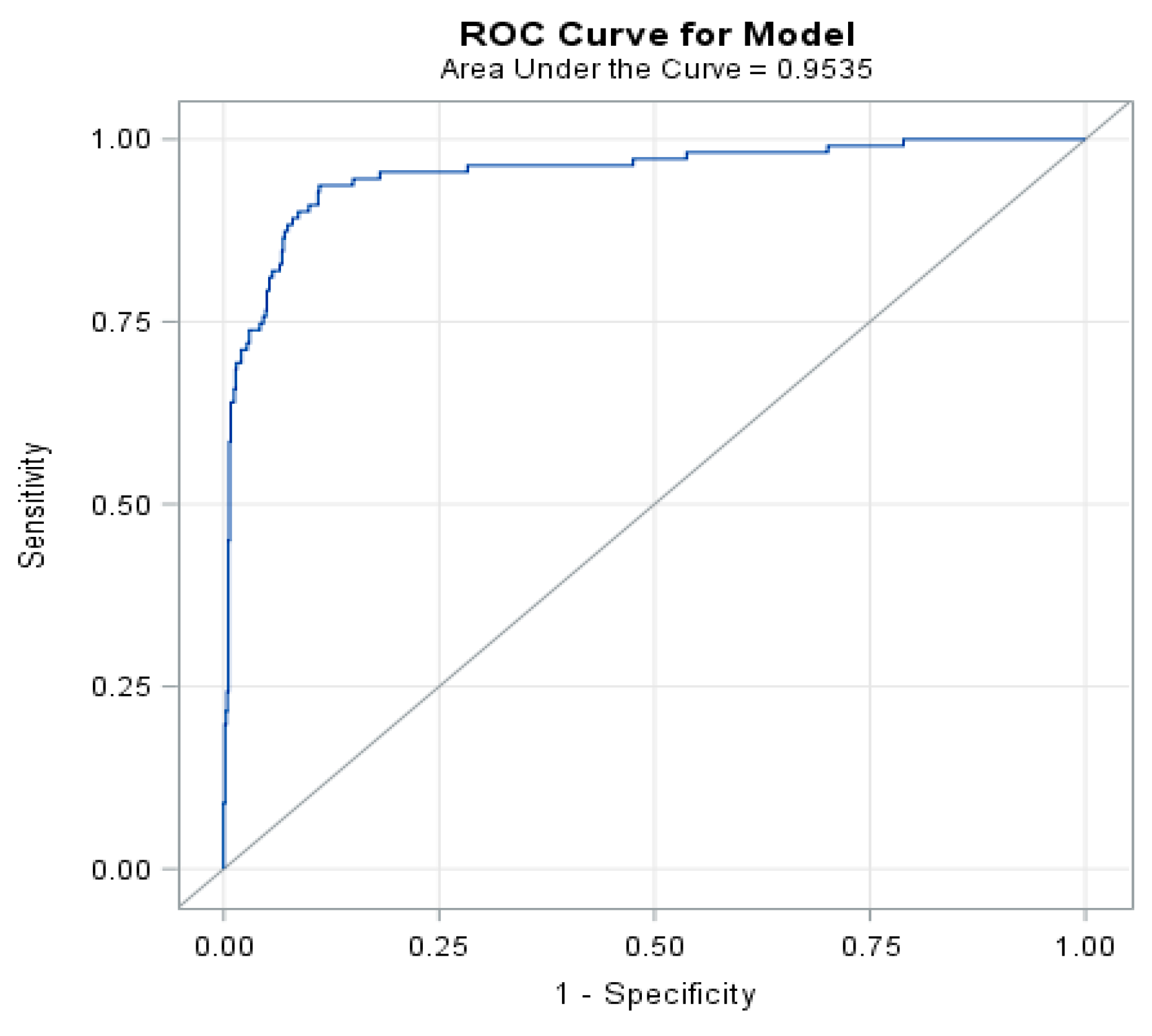
| Area | S.E. | Sig.b | Asymptotic 95% Confidence Interval | |
|---|---|---|---|---|
| Lower Bound | Upper Bound | |||
| 0.9535 | 0.012 | 0.000 | 0.930 | 0.977 |
| INTO | ||||
| FROM | 0 | 1 | Total | |
| 0 | Frequency | 733 | 6 | 739 |
| 1 | Frequency | 45 | 66 | 111 |
| Total | Frequency | 778 | 72 | 850 |
| Frequency Missing = 6 | ||||
© 2020 by the authors. Licensee MDPI, Basel, Switzerland. This article is an open access article distributed under the terms and conditions of the Creative Commons Attribution (CC BY) license (http://creativecommons.org/licenses/by/4.0/).
Share and Cite
Jenčová, S.; Štefko, R.; Vašaničová, P. Scoring Model of the Financial Health of the Electrical Engineering Industry’s Non-Financial Corporations. Energies 2020, 13, 4364. https://doi.org/10.3390/en13174364
Jenčová S, Štefko R, Vašaničová P. Scoring Model of the Financial Health of the Electrical Engineering Industry’s Non-Financial Corporations. Energies. 2020; 13(17):4364. https://doi.org/10.3390/en13174364
Chicago/Turabian StyleJenčová, Sylvia, Róbert Štefko, and Petra Vašaničová. 2020. "Scoring Model of the Financial Health of the Electrical Engineering Industry’s Non-Financial Corporations" Energies 13, no. 17: 4364. https://doi.org/10.3390/en13174364