Abstract
Aerodynamic drag and bearing friction are the main sources of standby losses in the flywheel rotor part of a flywheel energy storage system (FESS). Although these losses are typically small in a well-designed system, the energy losses can become significant due to the continuous operation of the flywheel over time. For aerodynamic drag, commonly known as windage, there is scarcity of information available for loss estimation since most of the publications do not cover the partial vacuum conditions as required in the design of low loss energy storage flywheels. These conditions cause the flow regime to fall between continuum and molecular flow. Bearings may be of mechanical or magnetic type and in this paper the former is considered, typically hybridized with a passive magnetic thrust bearing. Mechanical bearing loss calculations have been extensively addressed in the open literature, including technical information from manufacturers but this has not previously been presented clearly and simply with reference to this application. The purpose of this paper is therefore to provide a loss assessment methodology for flywheel windage losses and bearing friction losses using the latest available information. An assessment of windage losses based on various flow regimes is presented with two different methods for calculation of windage losses in FESS under rarefied vacuum conditions discussed and compared. The findings of the research show that both methods closely correlate with each other for vacuum conditions typically required for flywheels. The effect of the air gap between the flywheel rotor and containment is also considered and justified for both calculation methods. Estimation of the bearing losses and considerations for selection of a low maintenance, soft mounted, bearing system is also discussed and analysed for a flywheel of realistic dimensions. The effect of the number of charging cycles on the relative importance of flywheel standby losses has also been investigated and the system total losses and efficiency have been calculated accordingly.
1. Introduction
The majority of the standby losses of a well-designed flywheel energy storage system (FESS) are due to the flywheel rotor, identified within a typical FESS being illustrated in Figure 1. Here, an electrical motor-generator (MG), typically directly mounted on the flywheel rotor, inputs and extracts energy but since the MG is much lighter and smaller than the flywheel rotor, its aerodynamic drag and bearing loss contribution are much smaller than the flywheel rotor. The low contribution to losses of the MG are qualified later in the paper and it should also be noted that electromagnetic drag from the MG is not treated here since this is a subject which would be covered as part of the design and analysis of the MG for which there are numerous choices. There are also a number of choices for the bearings and these are discussed in-depth also in [1,2,3]. A low cost and simple bearing type commonly chosen is the mechanical bearing, typically rolling element with fluid lubrication and this type is considered in this paper.
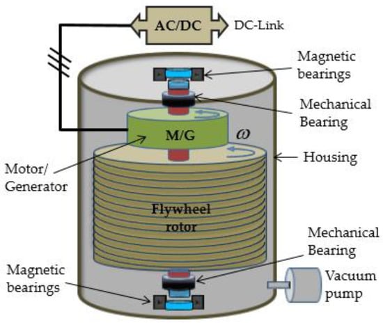
Figure 1.
Structure and components of flywheel energy storage system (FESS).
The main sources of loss in the flywheel rotor of the FESS are due to aerodynamic and bearing friction losses. The aerodynamic loss in a flywheel system, also called the windage loss, is due to the friction between the rotor part of the flywheel and surrounding air, whereas the bearing loss is generally dependent on the weight of the rotor and the type of lubricant used. The relative contribution of these losses to the total loss with reference to operating parameters is commented on later in the paper. Operation of flywheel systems at atmospheric pressure conditions would lead to high losses in terms of wasted energy and could result in overheating of the flywheel rotor [4]. To control the level of losses, the flywheel is enclosed in containment to create a vacuum environment because the losses reduce with a higher vacuum (i.e., absolute pressure), but not proportionally [5]. The losses can be fully eliminated by increasing the vacuum but its maintenance will be harder due to leaks and outgassing as a result of increased pressure ratio [6]. Outgassing occurs when solid materials and liquids (i.e., lubricating oil) release gas due to higher vacuum and lubricating oil required for the bearing system could even boil if the vacuum is too high. Notwithstanding the outgassing issue, maintaining a high level of vacuum is another challenge and requires constant operation of a vacuum pump, especially for the cases when high vacuum level is maintained using gas mixtures such as SF6 and He [7]. However, if the requirement for the vacuum level is not too high, it can be easily maintained with the low-cost solution of hermetically sealing the flywheel containment and pumping the casing down intermittently [8]. This mechanism will reduce the wear on the pump and the loss of power due to continuous running of the pump [9]. Depending on the effectiveness of the sealing, the pump can be taken off the system and vacuuming can be done every few years as a maintenance item [10] and under such operation, the energy consumption of the vacuum pump can be considered negligible.
The windage loss in a flywheel system itself is determined by the friction between the rotor and the air or gas surrounding it, which depends on the enclosure mechanism. It is approximately proportional to the cube of speed and can become intolerable if the pressure level is not controlled [4]. The windage losses can be reduced with low vacuum level which necessarily requires a casing to maintain a low-pressure environment. Reducing the pressure below atmospheric level, however, changes the surrounding gas medium to what is called the rarefied condition, a flow regime for which the aerodynamic loss must be calculated in another way. The fluid behaviour under rarefied conditions cannot be analysed by the methods of continuum fluid mechanics and must be predicted by the kinetic theory due to the effect of pressure on viscosity where the gas particles are located too far away from each other [11]. Operational regimes based on the kinetic theory are determined using statistical solutions or analytical methods. However, available literature addressing the aerodynamic losses in flywheel storage systems under rarefied vacuum conditions are quite limited and it is an area where this research explores in more detail with a presented methodology.
An analytical loss model of a novel outer rotor FESS validated based on measurements is presented in [12]. The design and analysis of the losses in a high-speed flywheel system are discussed in [13]. The former calculates the mechanical loss of the FESS while the latter studies the friction loss, core loss and the copper loss of the designed flywheel system, however, both papers ignore the losses due to windage. Mitigation of losses in FESS and analysis of different components of losses contributing to the total loss is discussed in [14]. The losses of a flywheel system operating with solar cells are studied in [15]. References [16,17,18,19] mainly address the losses in the electrical machine part of the FESS which are typically small in comparison to the losses in its rotor part. Reference [20] studies a FESS for satellite applications and presents an algorithm for controlling the flywheel losses. The calculation method for aerodynamic and mechanical friction losses in flywheel storage systems is discussed in [21]. However, both systems estimate the windage losses based on empirical equations valid for atmospheric pressure conditions which will give inaccurate results if the flywheel system operates in lower pressure levels or vacuum conditions. Suzuki et al. [22] discuss the effect of gas mixtures in reducing the aerodynamic losses in flywheel storage systems. The windage loss is determined using the coefficient of air resistance, but the effect of helium gas in rarefication of the vacuum chamber is not fully investigated. What is commonly absent in these papers is a methodology for determining the windage losses of vacuum-operated flywheel systems. The current research, therefore, uses the latest available information to propose an approach for estimation of aerodynamic drag coefficients for systems operating in rarefied gas conditions.
The losses due to bearing friction are generally determined by estimating the slip and shear stress within the interacting surfaces of the bearing. Despite the complexity of the available analytical models for predicting the bearing losses, the empirical approaches available in the literature as well as the technical information provided by the bearing manufacturers extensively address these losses. However, there are so many methods available with such a broad field of applications, the best methodology, suited for the specifics of flywheel application has not been easy to find. The methods available have therefore been reviewed to guide the reader interested in mechanical bearing losses in flywheels to a clear and simple method. Additionally, a good method for estimating bearing life has been identified and described.
The paper is structured to firstly address the determination of the flywheel standby losses, such losses consisting of the windage and bearing friction losses are considered in turn. The windage loss of flywheel systems in vacuum conditions is not widely addressed in the literature and is discussed in more detail here. The bearing friction loss is briefly described to make the context for estimation of the total standby losses, however, some design choices and the approach for selection of bearing systems is also presented in detail. Parametric type calculations are presented to illustrate typical values and tradeoffs for a flywheel of realistic dimensions and speed. This is followed by an analysis of the impact of the number of daily charge-discharge cycles on reducing the flywheel standby losses. The paper concludes with the calculation and analysis of the system total losses and efficiency concerning the standby losses and charging cycles of the flywheel system.
2. Flow Regimes and Windage Drag Coefficient
2.1. Rarefied Free Molecular Flow
The rarefication of aerodynamic flow types is normally classified as continuum flow, slip flow, transition flow and free molecular flow where the transition between each state is determined from the dimensionless Knudsen ( number as shown in Figure 2. It is defined as the ratio between the mean free path (λ) of a molecule and the dimension of the object under consideration which is the gap between the flywheel rotor and its surrounding containment [23].
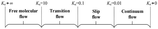
Figure 2.
Aerodynamic drag loss relative to the pressure at different air gaps.
The Knudsen number can also be calculated using the dimensionless parameters Mach number () and Reynolds number () as given by:
Such that:
where is the velocity, is the ratio of specific heats, is the viscosity, is the density, is the temperature, is the universal gas constant, and is the gap between the flywheel rotor and containment.
Flywheel storage systems require a reduced pressure inside the containment where the flow regime turns into rarefied free molecular flow due to the sufficiently spaced molecules. Hence the length scale of the flow (rotor-stator gap) will be much smaller than the mean free path of molecules, the surfaces collision of the molecules can be neglected, and the motion of molecules can be studied under Maxwellian distribution [24]. In free molecular flow the viscosity is varied in accordance with temperature and pressure and the continuum approximations based on fluid mechanics become invalid [11]. Solutions for such regimes are determined by kinetic theory using analytical or statistical methods. Analytical solutions of the flow of gases for the limiting cases of free molecular and continuum flow are generally derived using Boltzmann equation. However, approximations for a range of Knudsen numbers in the transition region between the two cases will be of great importance for more practical cases.
Approximate solutions of the Boltzmann equation including the intermediate region have been developed by several authors building upon the early work of Millikan [25]. The air friction due to cylindrical surfaces moving rapidly in a low-pressure environment is analysed in [26]. Authors of [27,28] have developed approximations for free molecular drag in cylindrical Couette flow. The drag force on objects in the transition region studied based on the kinetic theory is presented in [29]. An approach with reference to the Maxwell-Boltzmann equation and kinetic theory of gas flows is developed in [30]. It is shown to be valid for the entire range of Knudsen numbers, however, the method is fairly complex and is limited concerning non-linearity of gases in rarefied conditions including the behaviour of gases due to temperature variations. The current research proposes a methodology for the approximation of aerodynamic losses of cylindrical flywheels operating in rarefied mediums as developed in reference to the work of Beck [31] and Alofs [32]. The windage losses of an intermediate speed (10–20 krpm) steel-rotor flywheel system are estimated based on the mathematical expressions developed for windage drag coefficients and shear stress of cylindrical flywheels.
2.2. Windage Drag Coefficient at Low-Pressure Medium
Beck was the first to derive an expression for shear stress under rarefied condition between two infinitely extended plates a and b with a separation distance d and a constant relative velocity V as given by [31]:
where is the shear stress between the two surfaces a and b, m is the molecular mass and n is the number density.
The value of in Equation (4) is dependent on the Knudsen number and is valid when the temperature difference between the two plates is neglected .
An object with relatively large velocity moving through a fluid will experience a force as given by:
where the drag coefficient is a dimensionless quantity that is a function of speed, roughness and geometry of the object. Using Equation (6), the drag coefficient of cylindrical surfaces as a function of shear stress can be represented by:
Substituting Equations (4) and (5) in Equation (7) and simplifying gives:
Equation (8) can be further expanded by substituting Equations (1) and (7) to express the shear stress of cylindrical objects as a function of the Reynolds number () and Mach number () as given by:
Hence, using the derived shear stress expression, the drag loss of a cylindrical flywheel with radius r and length h can be calculated by:
The derived expression can be used to estimate the windage power loss of flywheel systems in rarefied gas environments. The limitations and the level of accuracy of Equation (11) at different pressure levels are further investigated by accommodating tangential momentum accommodation coefficient () in the expression for shear stress.
Bowyer and Talbot [27] have developed a formula for shear stress in cylindrical coquette flow for rarefied gases valid for the condition of complete accommodation () as given by:
Similarly, Kennard [28] has also developed an expression for plane Couette flow in rarefied gas conditions valid for other values of as given by:
An expression for windage drag of cylindrical surfaces in free molecular flow including the momentum accommodation coefficient can be derived by combining Equations (12) and (13).
Therefore, an expression for drag loss due to windage in cylindrical flywheels accommodating () and ( is developed by substituting Equation (14) in (10):
Equation (15) can accommodate different values of and its validity for a wide range of Knudsen numbers has been tested by the experimental results of Alofs and Springer [32]. Analysis of flywheel windage losses in this study is performed using Equation (11) and compared with the results produced based on Equation (15) to indicate the level of accuracy and correlation of both methods at different pressure levels.
3. Bearing Friction Losses
The overall losses in ball bearings can be estimated by considering the slip and shear stress at interacting surfaces within the bearing. However, predicting the torque and power loss of bearing through analytical models is complex and still limited in the accuracy in some applications. This is due to the level of difficulty associated with satisfactorily quantifying the relationship between the state of lubricant within the bearing cavity and the applied lubricant conditions. Therefore, control of the amount of lubricant in the cavity to the amount of lubricant supply is determined empirically as favoured in industry and also by bearing manufacturers [33]. In this work, an empirical approach developed by Palmgren [34] is used to estimate the bearing friction losses in the proposed flywheel system. He determined the empirical factors for all types of rolling bearings and developed equations for the frictional torque. According to Palmgren, the torque of a rolling bearing () consists of two components: one speed dependent () and the other load dependent () [35].
The load term is determined by the bearing type and load:
where is the load applied on the bearing (N), is the pitch circle diameter of the rolling element (inches) and is a factor dependent on bearing design and relative load that can be obtained by:
where is the static equivalent load (N), is the static load rating (N), are load torque factors determined experimentally (see Appendix A). The static equivalent load is a theoretical load that is assumed to produce a contact stress equivalent to the maximum stress when the bearing is operating under actual practical conditions.
The load factor in Equation (17) is dependent on magnitude and direction of the applied load on bearing as given by:
Finally, the speed-dependent component of the bearing torque is the combined effect of the speed and viscous shearing of the type of lubricant used for the bearing:
where is the axial load (N), is the radial load (N), is the bearing speed (rpm), is the kinematic lubricant viscosity (centistokes) and is a factor dependent on bearing type and mode of lubrication (Table A2).
3.1. Bearing Sizing and Selection
Selection of bearing for use in flywheel applications is dependent on a combination of parameters including bearing static and dynamic load, operational speed and an acceptable level of maintenance. In addition to supporting the flywheel weight and dynamic forces, the selected bearing is also required to have a satisfactory life with low maintenance and an acceptable level of losses. Suitable bearing types for high-speed applications are hydrodynamic bearings, airfoil bearings, different types of magnetic bearings and rolling element bearings [36]. Hydrodynamic bearings are suitable for high-speed applications under vibrating conditions and airfoil bearings can operate at high speed under high-temperature levels as they do not require lubrication and the bearing surfaces are kept apart by pressurised air. However, the former needs special treatment of the oil lubrication system and the latter requires pressurised air which makes them unsuitable for flywheels due to their requirements and a higher level of costs. Since the flywheel is operating in a vacuum and to avoid leakage and friction loss due to shaft seals, magnetic bearing and rolling element types are the best choices available. However, magnetic bearings and particularly active magnetic type are expensive and complex and cannot withstand larger acceleration and gyroscopic forces. They also need rolling bearings as back up in case of power failure.
With the above considerations and as per bearing manufacturers recommendations, the flywheel rotor in this study is balanced by a combination of passive magnetic bearing and radial ball bearings as shown in Figure 3. The rotor of the proposed flywheel system is a one-piece steel cylinder machined at either end to the required diameter and supported by two angular contact ball bearings on both sides of the shaft.
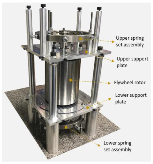
Figure 3.
Configuration of the proposed flywheel.
The majority of the weight is vertically levitated by the passive magnetic bearing which theoretically has no losses and the two relatively small diameter ball bearings are used to radially stabilise the spinning rotor. In order to keep the rotor spinning around its mass rather than geometric axis, soft springs are mounted on ball bearings to accommodate for any small out of balance displacement as shown in Figure 4. This minimizes the force on the bearings so they can be reduced in size for lowest loss. Each bearing is housed in a steel cap with evenly spaced six holes on its periphery. The bearing caps on top and bottom are connected to the set of six springs, which are secured at the holes on the bearing cap on one side and to the bolts of adjustable steel ring on the other side
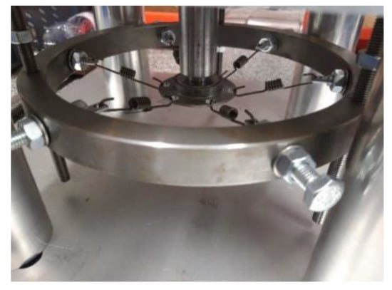
Figure 4.
Bearing balanced by flexible six-spring set.
The vertical position of the steel ring on top and bottom support plates can be adjusted by means of the three studs. The passive magnetic bearing at the top, on the other hand, is mounted between the flywheel rotor and the top supporting plate.
Angular contact ball bearings are generally a good choice and give excellent life if the bearing is maintained well and the temperature is not allowed to exceed the limits of the lubricant. Calculation of the bearing life and lubrication selection are discussed in upcoming subsections to explain and justify the choices for selection of a low maintenance option with satisfactory operating lifetime.
3.2. Bearing Lubrication Selection
The type of lubrication in rolling element bearings determine the operating temperature as well as the speed limit and bearing losses. Oil lubrication allows the highest speed operation but with the downside of requiring frequent maintenance and additional equipment for oil pumping. High-pressure oil feed system is also a good alternative to control the temperature, but its sophisticated oil supply system needs a high-pressure pump with filter and oil cooler adding to the overall cost of the system. Grease is another option and serves best in terms of maintenance requirements and life expectancy, however, it has a lower cooling effect and limits the operational speed in comparison to oil lubrication. Taking into account the important factors such as lubricant viscosity, cooling effect, quantity and mode of supply, and vapour pressure level of the lubricant, a nominal lubrication method preferred in the majority of the bearing systems is either oil mist or grease lubrication method [33].
The type of lubricant for the two radial bearings supporting the flywheel is selected by considering the above requirements. The lower bearing will have the highest load and acts as a register bearing by taking the net axial load. Therefore, it is oil-lubricated by creating an oil mist so its temperature is kept at the lowest. The top ball bearing, on the other hand, will be grease lubricated because getting an oil mist to this bearing is difficult and will possibly develop an oil mist around the flywheel rotor which will further contribute to windage losses. The selection of grease lubricant can be justified since the speed of the steel rotor is not particularly high, and also the top bearing is lightly preloaded by the attached springs which will not experience significant load variations. Hence heat generation and temperature control will not be an issue.
3.3. Bearing Life
Bearing life as defined by the bearing manufacturers is the duration that it can safely endure load under rotating conditions. The rolling surfaces experience a high number of cyclic stresses that can lead to cracks under or at the surface which will cause material failure on the surface of the rolling elements and would leave a pit. Signs of fatigue pit can be detected in the form of noise or vibration and this indication is considered to be the end of bearing life. However, this failure mode is still safe and the bearing can operate for sufficient time before remedial action is taken [33]. For flywheel applications where the maintenance requirement is favoured to be at a minimum and bearing breakdown or even the failure mode could lead to a catastrophic, fatigue life calculation becomes an important step in bearing selection and design process.
A simple and widely used calculation method for the bearing fatigue life is the basic rating life. It is defined as the total number of operating hours completed by a number of selected bearings (operating individually and under the same conditions) when 10% of them fail to function due to flaking [35]. The following relation calculates basic rating life for ball bearings as a function of bearing load:
where (millions of revolutions) is the basic rating life (at 90% reliability), (operating hours) is the basic rating life (at 90% reliability), is basic dynamic load rating (N), is the equivalent dynamic load (N), is the rotational speed (min−1) and is the exponent of the life Equation (3 for ball bearing, 10/3 for roller bearing). The equivalent dynamic load () is a hypothetical load with constant magnitude and direction to account for the actual dynamic load that is applied on the bearing in practical conditions. It consists of a radial component for radial bearings and an axial component for thrust bearings as calculated using the following general equation:
where is the dynamic radial load factor and is the dynamic axial load factor (Table A3).
The rating life for modern high-quality bearings, however, will be considerably different and it will deviate from the actual service life in a given application because many factors such as lubrication, errors in bearing design and selection, improper mounting, inadequate maintenance and environmental conditions are not taken into account in calculating the bearing basic life. Since bearing life calculations considering these factors are quite computational and require test data, a simplified approach practised by many bearing manufacturers is the inclusion of modification and adjustment factors to complement the basic rating life equations and give an estimation of the fatigue life rating close to practicality. Hence, the modified life equations based on the adjustment factors proposed by manufacturer SKF take the form [37]:
where (million revolutions) is the modern rating life (at 100—n% reliability), is the life modification factor, (operating hours) is the rating life (at 100—n% reliability) and is the life adjustment factor for reliability (Table A4).
4. Results and Analysis
4.1. Aerodynamic Drag Losses
The specifications of the flywheel system including the air density values at 20 °C and atmospheric pressure conditions are provided in Table 1. The standby windage loss of the system at different speeds and pressure levels is estimated with help of Equations (1)–(3) and power loss expressions due to windage drag as derived and presented in Equations (11) and (15).

Table 1.
Flywheel specifications and air properties.
Results of windage loss calculations for a constant air gap of 1 mm and a range of pressure levels between 0.001–100 Pa are presented in Figure 5. Each pressure level is tested for different speeds ranging between 1000–300,000 rpm. The considered flywheel system has an operating speed range of 10,000–200,000 rpm and pressures of 10 Pa and 100 Pa will not be reached due to vacuum operation, however, calculations beyond these limits are performed for a better comparison of the methods explained and as an indication of the rate how these losses increase with pressure and speed.
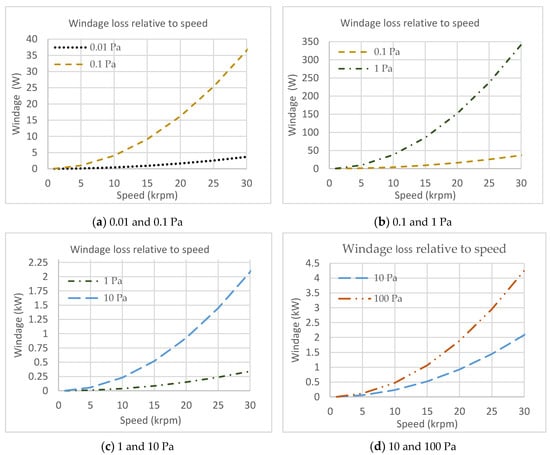
Figure 5.
Aerodynamic drag loss relative to speed and pressure.
The results of loss estimations show that windage losses increase exponentially and become unacceptable if the pressure level is not controlled, which justifies the need for a vacuum container. In addition to the effect of pressure and speed on windage losses, the air gap variations between the flywheel rotor and container are also studied in this calculation method and the windage losses at different air gaps ranging between 1–5 mm are shown in Figure 6. The speed range is further extended to 40,000 rpm since the air gap effect on aerodynamic loss is more evident at larger speeds.
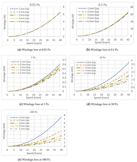
Figure 6.
Windage loss relative to pressure and speed at different air gaps—method 1 (without ).
The estimation of losses at lower pressures shows that the effect of air gap variations is negligible and the windage losses remain the same for all air gaps. If the pressure level is increased to 1 Pa, the losses slightly decrease as the air gap increases. This is evident in higher pressures (10 Pa and 100 Pa) where the losses are significantly increased with the reduction of the air gap. For instance, changing the air gap from 5 to 1 mm at 2000 rpm speed will increase the losses by approximately 590 W at 10 Pa and 1470 W at 100 Pa, respectively.
Since the proposed calculation method is developed for vacuum conditions, its accuracy and limitations for higher pressures need to be evaluated. Hence, as shown in Figure 7, further results are produced using the method derived in Equation (15) where the momentum accommodation coefficient (σ) is included in the calculations and all pressure levels are accommodated.
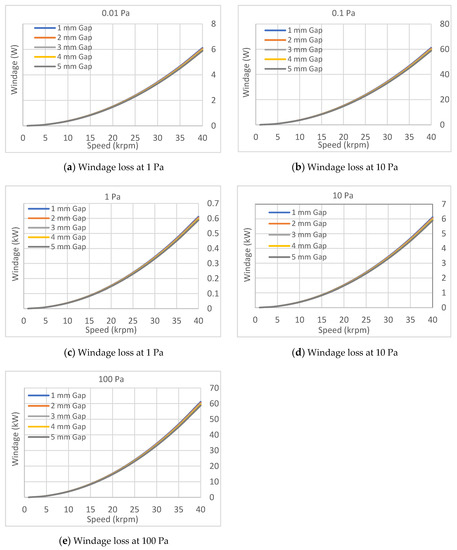
Figure 7.
Windage loss relative to pressure and speed at different air gaps–Method 2 (with ).
The results obtained show that both calculation methods give similar and accurate results at lower pressures and are hardly affected by the air gap differences. As the pressure increases beyond 1 Pa, windage losses in method 1 change significantly with different air gaps although the losses based on method 2 show consistency and close correlation for the entire range of air gap values.
Method 1 is valid for rarefied gas conditions with low-pressure level, hence at large pressures, any small increase in the air gap will contribute to rarefication of the medium and the windage loss will be reduced. For example, a change of air gap from 1 to 5 mm at 20,000 rpm will reduce the windage loss by approximately 35 W at 1 Pa (Figure 6c), 590 W at 10 Pa (Figure 6d) and nearly 1.5 kW at 100 Pa (Figure 6e), respectively. Therefore, both methods are valid for the entire range of Knudsen numbers and can be used for calculation of windage losses in flywheel systems. However, in method 1 the air gap deviation is also taken into account and is quite useful for the cases of variable gap between the rotor and surrounding containment.
The statement made earlier in the introduction that the MG makes a low contribution to the losses can be justified given that the calculation methods for windage losses have been described. For the flywheel described in Table 1, the MG would have a power output in the order of 10′s kW. Taking a maximum power of 100 kW and assuming a MG rotor peripheral speed of 180 m/s and a range of magnetic shear stress of 0.001–100 Pa, the rotor, radial flux, will have a diameter and length of 172 and 206 mm, respectively. For a 1 mm air gap, the windage losses of the flywheel rotor and MG are calculated according to the methods described and compared in Table 2. The ratio of MG windage loss to flywheel rotor is shown to be approximately 3% for all pressure levels and is therefore small enough to be neglected.
Table 2.
Results of windage loss for flywheel rotor and MG relative to the pressure.
Finally, the windage loss for continuum and molecular flow regimes as a function of the flywheel pressure level is now shown in Figure 8. The losses in the molecular region are calculated based on rarefied gas conditions using the approximation methods developed in this work, whereas for the case of continuum regimes, the calculation methods for atmospheric conditions are used. For each flow regime, it is shown that the level of losses for the two conditions of 1 and 5 mm radial gap is quite close and not significantly affected by changing the pressure level. Although the flywheel system will be operating in molecular regime due to vacuum conditions and this will be well below the 10 Pa pressure level, to the author’s best knowledge, there is no theory or test available for the windage losses in the transition region between continuum and molecular flow regimes and these losses are usually calculated by interpolation method.
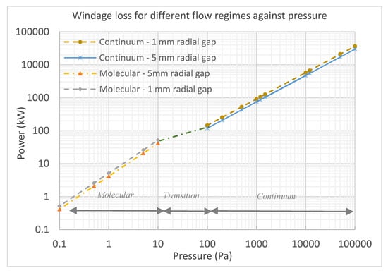
Figure 8.
Windage loss against pressure for continuum and molecular flow regimes.
4.2. Bearing Friction Losses
The static and dynamic loads, as well as the specifications of the bearing assembly of the proposed flywheel system, are summarised in Table 3. The lower bearing will have the highest load by taking the net axial load of approximately 5% of the rotor weight including the weight of the integrated MG. The top bearing will be supported by the attached springs, and a light preload as recommended by the bearing manufacturers will be considered for this bearing.
Table 3.
Bearing specifications and static and dynamic loads.
The radial load on the bearings is not fixed and is estimated using ISO 1940/1 for a balance quality grade of G0.4 [38]. This gives an unbalanced force of approximately 260 N although this is unlikely to be as high as this since it will be significantly reduced due to the presence of soft mounting of the bearing outer races using springs. Opposite to the case of axial loads, most of the radial load will act on the top bearing since the length of the integrated MG moves the lower bearing further away from the flywheel rotor. Hence, 160 N for the top bearing and 100 N for the lower bearing are assumed. The effect of springs on the overall system dynamics is analysed based on the considerations that the flywheel rotor is axisymmetric and rigid, and the deviations of the centre of gravity of the flywheel are small. The rigidity of the rotor can be justified in reference to the assumption that if the rotor stiffness is considerably higher than the stiffness of the bearing support system, the rotor behaves as a rigid body [39]
The type and specification of the bearings including the factors and parameters for bearing life calculations are presented in Table A1, Table A2, Table A3, Table A4, Table A5 and Table A6 in Appendix A. Considering the bearing type and lubrication method described above, the load-dependent torque and speed-dependent torque on the bearings are determined by substituting the relevant parameters into Equations (17) and (20). The losses due to both bearings supporting the flywheel rotor for different operating speeds are presented in Table 4.
Table 4.
Results of bearing standby loss calculations.
Most of the estimated losses occur on the top bearing and the majority comes from the speed-dependent loss component. This is partially due to larger radial load on this bearing but it is mainly related to the type and mode of lubrication. As the speed increases, the speed-related losses for the top bearing increases much greater compared to the load-related losses. This is not the case for the lower bearing since it is oil-lubricated and the viscosity and mode of lubrication contributions are small. Hence, the type of lubrication determines the implication of load-related and speed-related losses.
Bearing life calculations for both bearings operating at different speeds are shown in Table 5. In contrast to the strong dependency of lubrication type on the bearing losses, the applied load mainly affects the bearing life but the type of lubrication has less of an effect. It is dependent on the equivalent load and the type of bearing. Since the same type of bearing has been selected for both the top and lower bearings, the larger equivalent load on the lower bearing greatly reduces its estimated lifetime. The equivalent load on the lower bearing is 40% higher than the top bearing. If we compare both bearings at 20,000 rpm, the estimated basic life of the top bearing is 178,000 h while that of the lower bearing is 38,000 h. The modified rating life of the top and lower bearings are 284,000 h and 98,000 h, respectively. Therefore, despite the lower bearing having a relatively less viscous lubricant compared to the grease-lubricated top bearing, an increase of 40% in its equivalent load will reduce its basic lifetime by 78% and modified rating life by 65%. Additionally, factors such as dynamic load rating (C) and fatigue load limit (Pu) will also affect the bearing life rating. Selecting a different type of bearing with lower C value will have a shorter bearing life rating.
Table 5.
Results of bearing life calculations.
4.3. Total Losses and Efficiency
In order to determine the overall efficiency of the system, total standby losses including windage and bearing friction losses must be taken into account. The flywheel self-discharge rate increases nonlinearly as the speed and pressure increase. The windage losses vary with pressure and speed although bearing losses are only speed dependent. Hence the combined run-down losses will be a combination of different powers of speed due to multiple power loss expressions () included in the calculations. Air gap variations will also have a significant effect at higher pressure, hence, a gap of 1 mm is considered as a worst case. The standby self-discharge rate of the flywheel system at three different pressures of 0.01, 0.1 and 1 Pa is shown in Figure 9. The flywheel is considered to be initially fully charged and running at 20,000 rpm, and then left on standby mode for 24 h without any further recharging.
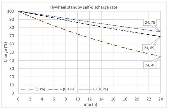
Figure 9.
Flywheel standby discharge rate in 24 h.
The 24-h run down losses at lower pressures are smaller and gives 25% discharge at 0.01 Pa and approximately 30% discharge and 0.1 Pa. When the pressure is increased to 1 Pa, the discharge rate is almost doubled to 55% and approximately 2740 Wh of energy is lost in 24 h. This is because of the exponential increase of the windage losses with respect to rising pressure. At lower pressures, the windage losses are insignificant and bearing friction losses dominate the standby losses. At 1 Pa and at higher speeds, however, the windage losses increase substantially while the rate of change of bearing losses is less pronounced. Since the flywheel will be operating in a vacuum and a pressure of 0.01 Pa could be easily maintained, a pressure of 1 Pa can be avoided and considered as the maximum operating pressure limit. What this analysis illustrates is that the windage loss can be strongly controlled by changing the pressure whereas there are fewer opportunities to reduce the bearing loss. It therefore makes sense to set the pressure such that the windage losses are of a similar order of magnitude to the bearing losses rather than choosing to reduce the vacuum pressure to the point of diminishing returns given the cost of maintaining a harder vacuum. In addition, this analysis is performed based on the assumption that the flywheel performs only one charge-discharge cycle per day and then switches to standby mode for the course of 24 h. Considering this, if the number of cycles per day is increased, the percentage of energy loss during standby periods will become smaller as shown in Table 6.
Table 6.
Flywheel standby discharge rate relative to the number of cycles.
The proposed flywheel system is C2 rating (5 kWh, 10 kW) and takes 30 min charge-discharge time between 50% charge to fully charged and back to 50% state of charge. For 10 cycles per day, the flywheel will be idling for 19 h and this gives 47% discharge rate if the pressure reaches the maximum of 1 Pa. For the same pressure, the self-discharge rate can be reduced to an acceptable level of 25% for 30 cycles and this is further improved to 12% and 10% if the pressure is reduced to 0.1 and 0.01 Pa, respectively. The standby losses will be far reduced for 40 and 45 cycles but this will not be realistic since the maximum possible number of cycles per day is 48 and the flywheel would hardly rest. A compromise must be made between the number of cycles and standby losses based on the level of pressure in the vacuum. For instance, the self-discharge rate of 25% can be reached for 10 cycles at 0.1 Pa or 30 cycles at 1 Pa. Therefore, 10 cycles per day is considered as an acceptable compromise for calculating the run down losses and system efficiency. This will give a self-discharge rate of 4.7% per cycle in the extreme conditions of 1 mm air gap and 1 Pa pressure.
The efficiency of the system can be calculated considering the system conversion efficiency during charging () and discharging () which are also dependent on the energy losses in the electrical machine and related power electronics. The overall efficiency per cycle of the flywheel system () including the run down losses can be calculated by assuming an efficiency of 98% for power electronics and 95% for the MG (electrical machine) giving an overall round trip efficiency of approximately 83%. Accordingly, the maximum standby losses of 230 W can be confirmed by combining the windage losses with the bearing friction losses for an operating speed of 20,000 rpm. The remaining operational losses are approximately 310 Wh per cycle.
5. Conclusions
This paper has described a methodology for estimation of standby losses in flywheel storage systems operating in vacuum conditions, which is an area previously not addressed in the literature in a clear manner focused on this application.
Calculations of aerodynamic and bearing friction losses were performed at different speeds and pressures to show the substantial level of losses in flywheel systems operating in atmospheric conditions and the need for maintaining a vacuum environment. For the case of vacuum environments with rarefied gas conditions, two different windage loss calculation methods were developed, compared and justified by performing a comprehensive analysis of the proposed flywheel system. The findings of the research showed that both methods represent quite a close correlation for pressure levels below 1 Pa, but will show some disparity for pressures higher than 1 Pa. Nevertheless, method 1 exhibited a satisfactory level of consistency and also includes air gap variations.
Bearing friction losses and life calculations concerning loading conditions, mode of lubrication and maintenance requirements are determined using empirical approaches recommended by the bearing manufacturers. It was shown that the bearing losses are strongly dependent on lubrication type and not majorly affected by the applied load. In contrary, the loading condition mainly challenges the effective life of the bearing and the type of lubrication has less of an effect.
The total loss and efficiency of the proposed flywheel system were determined based on the results of bearing friction and windage losses. Analysis of the effect the flywheel operating cycles indicated that the standby losses can be minimised by increasing the number of charge-discharge cycles, however, a realistic and practical system requires a compromise between the number of cycles and standby losses. Therefore, 10 cycles per day was considered as an acceptable compromise for calculating the run down losses and system efficiency. It was shown that the system will incur maximum standby losses of 230 W in 10 cycles while the remaining operational losses will be 310 Wh per cycle.
The mathematical equations and methodology developed for estimation of windage drag coefficients are proposed for estimation of aerodynamic windage losses in flywheel systems operating in full or partial vacuum conditions. Further research will focus on the method of windage loss estimations in the transition flow regime since there is no theory available for this region and mostly the calculations are performed by using interpolation between continuum and molecular flow regimes. Future research will be directed on experimental verification of the theoretical methods for estimation of flywheel energy storage system losses as presented in this article.
Author Contributions
All authors have contributed to the idea behind the work. M.E.A. has contributed on the conceptualisation, methodology and preparation of the original draft. K.R.P. has done the review and supervision. All authors have read and agreed to the published version of the manuscript.
Funding
This work has been supported by European Union’s Erasmus Mundus programme and City, University of London’s internal funding.
Acknowledgments
We thank European Union’s Erasmus Mundus programme and City, University of London’s internal funding.
Conflicts of Interest
The authors declare no conflict of interest.
Appendix A
The static equivalent load is a theoretical load that is assumed to produce contact stress equivalent to the maximum stress when the bearing is operating under actual practical conditions. It is calculated using Equation (A1) and the greater of the two values should be accounted for the static equivalent load on radial bearings.
where is the radial load (N), is the axial load (N), is the static radial load factor and is the static axial load factor (Table A2).
Table A1.
Values of permissible static load factor fs [33].
Table A1.
Values of permissible static load factor fs [33].
| Operating Conditions | ||
|---|---|---|
| Ball Bearings | Roller Bearings | |
| Low-noise applications | 2.0 | 3.0 |
| Bearings subjected to vibration and shock loads | 1.5 | 2.0 |
| Standard operating conditions | 1.0 | 1.5 |
Table A2.
Values of the load factor, torque factor and lubrication factor [33,34,35].
Table A2.
Values of the load factor, torque factor and lubrication factor [33,34,35].
| Load Torque Factors | |||||||
|---|---|---|---|---|---|---|---|
| Bearing Type | Xs | Ys | z | y | Oil Mist/Injection | Oil Bath /Grease | Oil Bath/Jet |
| Single row radial | 0.6 | 0.5 | 0.0007 | 0.55 | 0.7–1.0 | 1.5–2.0 | 3.0–4.0 |
| Angular contact, (α = 15°) | 0.5 | 0.47 | 0.001 | 0.33 | 1.0 | 3.0 | 6.0 |
| α = 20° | 0.5 | 0.42 | 0.001 | 0.33 | 1.0 | 3.0 | 6.0 |
| α = 25° | 0.5 | 0.38 | 0.001 | 0.33 | 1.0 | 3.0 | 6.0 |
| α = 30° | 0.5 | 0.33 | 0.001 | 0.33 | 1.0 | 3.0 | 6.0 |
| α = 35° | 0.5 | 0.29 | 0.001 | 0.33 | 1.0 | 3.0 | 6.0 |
| α = 40° | 0.5 | 0.26 | 0.001 | 0.33 | 1.0 | 3.0 | 6.0 |
| Angular contact double row | - | - | - | - | 2.0 | 6.0 | 9.0 |
The basic dynamic load ( is a constant load on the bearing that it can withstand for a rating life of one million revolutions. The factor is an adjustment factor when calculating the modified life of the bearing. It shows the percentage of the failure when the bearing completes millions of revolutions. The value of is a function of viscosity ratio () for lubrication condition, the level of contamination in the bearing () and the ratio of the fatigue load limit to the acting bearing equivalent load (). These values are obtained from the data sheets provided by bearing manufacturers.
Table A3.
Values of dynamic load factor Xd and Yd for angular contact bearings [35].
Table A3.
Values of dynamic load factor Xd and Yd for angular contact bearings [35].
| Nominal Contact Angle | e | |||||
|---|---|---|---|---|---|---|
| Xd | Yd | Xd | Yd | |||
| 15 | 0.178 | 0.38 | 1 | 0 | 0.44 | 1.47 |
| 0.357 | 0.40 | 1.40 | ||||
| 0.714 | 0.43 | 1.30 | ||||
| 1.070 | 0.46 | 1.23 | ||||
| 1.430 | 0.47 | 1.19 | ||||
| 2.140 | 0.50 | 1.12 | ||||
| 3.570 | 0.55 | 1.02 | ||||
| 5.350 | 0.56 | 1.00 | ||||
| 18 | - | 0.57 | 1 | 0 | 0.43 | 1.00 |
| 25 | - | 0.68 | 1 | 0 | 0.41 | 0.87 |
| 30 | - | 0.80 | 1 | 0 | 0.39 | 0.76 |
| 40 | - | 1.14 | 1 | 0 | 0.35 | 0.57 |
| 50 | - | 1.49 | - | - | 0.73 | 1 |
| 55 | - | 1.79 | - | - | 0.81 | 1 |
| 60 | - | 2.17 | - | - | 0.92 | 1 |
Table A4.
Values of the life adjustment factor [37].
Table A4.
Values of the life adjustment factor [37].
| Reliability | Failure Probability | SKF Rating Life | Factor |
|---|---|---|---|
| n | |||
| % | % | Millions revolution | - |
| 90 | 10 | 1 | |
| 95 | 5 | 0.64 | |
| 96 | 4 | 0.55 | |
| 97 | 3 | 0.47 | |
| 98 | 2 | 0.37 | |
| 99 | 1 | 0.25 |
Table A5.
Angular contact super precision ball bearing specifications [37].
Table A5.
Angular contact super precision ball bearing specifications [37].
| Bearing SKF 7005 CD/P4A | Principle Dimensions | Basic Load Ratings | Fatigue Load Limit | Max Speed | |||
|---|---|---|---|---|---|---|---|
| Bore Diameter | Outside Diameter | Width | Dynamic | Static | |||
| d | D | B | C | CS | Pu | ||
| mm | mm | mm | kN | kN | kN | krpm | |
| Top bearing (Grease lubricate) | 25 | 47 | 12 | 9.56 | 5.2 | 0.22 | 36 |
| Lower bearing (Oil lubricate) | 25 | 47 | 12 | 9.56 | 5.2 | 0.22 | 56 |
Table A6.
Values of life modification factor [37].
Table A6.
Values of life modification factor [37].
| Actual Operating Viscosity | Rated Viscosity | 1 | ||||||
|---|---|---|---|---|---|---|---|---|
| Oil-Mist (mm2/s) | Grease (mm2/s) | ndm | ||||||
| 4 | 40 °C | 100 °C | 40 °C | 100 °C | mm2/s | |||
| Top bearing | - | - | 26 | 4.5 | 7 | 0.64 | 0.4 | 2.5 |
| Lower bearing | 16 | 4 | - | - | 7 | 0.57 | 0.5 | 4 |
1 Calculated based on the specifications and diagrams provided by SKF.
References
- Kailasan, A.; Dimond, T.; Allaire, P.; Sheffler, D. Design and Analysis of a unique energy storage flywheel system—An integrated flywheel, motor/generator, and magnetic bearing configuration. J. Eng. Gas Turbines Power 2015, 37, 1–10. [Google Scholar] [CrossRef]
- Mao, C.; Zhu, C. Vibration control for active magnetic bearing rotor system of high-speed flywheel energy storage system in wide range of speed. In Proceedings of the 2016 IEEE Vehicle Power and Propulsion Conference (VPPC), Hangzhou, China, 17–20 October 2016. [Google Scholar]
- Zhang, C.; Tseng, K.J. A novel flywheel energy storage system with partially self-bearing flywheel rotor. IEEE Trans. Energy Convers. 2007, 22, 447–487. [Google Scholar] [CrossRef]
- Pyrhonen, J.; Jokinen, T.; Hrabovcova, V. Chapter 9: Heat transfer. Design of Rotating Electrical Machines; John Wiley & Sons, Ltd.: West Sussex, UK, 2008; pp. 477–482. [Google Scholar]
- Liu, H.P.; Werst, M.D.; Hahne, J.J. Investigation of windage splits in an enclosed test fixture having a high-speed composite rotor in low air pressure environments. IEEE Trans. Magn. 2005, 41, 316–321. [Google Scholar] [CrossRef]
- Werst, M.D.; Hahne, J.J.; Liu, H.P.; Penney, C.E. Design and testing of a high-speed spin test for evaluating pulse alternator windage loss effects. IEEE Trans. Magn. 2003, 39, 389–393. [Google Scholar] [CrossRef]
- Kobuchi, J.; Oobayashi, K.; Shimada, R. Windage loss reduction of flywheel/generator system using He and SF/sub6/gas mixtures. In Proceedings of the 32nd Intersociety Energy Conversion Engineering Conference, IECEC-97 (Cat. No.97CH6203). Honolulu, HI, USA, 27 July–1 August 1997. [Google Scholar]
- Amiryar, M.E.; Pullen, K.R. Assessment of the Carbon and Cost Savings of a Combined Diesel Generator, Solar Photovoltaic, and Flywheel Energy Storage Islanded System. Energies 2019, 12, 3356. [Google Scholar] [CrossRef]
- Asami, F.; Miyatake, M.; Yoshimoto, S.; Tanaka, E. A method of reducing windage power loss of a high-Speed motor using a viscous vacuum pump. Precis. Eng. 2017, 48, 60–66. [Google Scholar] [CrossRef]
- Amiryar, M.E.; Pullen, K.R. Development of a High-Fidelity Model for an Electrically Driven Energy Storage Flywheel Suitable for Small Scale Residential Applications. J. Appl. Sci. 2018, 8, 453. [Google Scholar] [CrossRef]
- Thoolen, F.J. Development of an advanced high speed flywheel energy storage system. Eindh. Univ. Technol. 1993. [Google Scholar] [CrossRef]
- Schneider, M.; Rinderknecht, S. System Loss Measurement of a Novel Outer Rotor Flywheel Energy Storage System. In Proceedings of the International Electric Machines and Drives Conference (IEMDC), San Diego, CA, USA, 11–15 May 2019. [Google Scholar]
- Zhang, C.; Tseng, K.J.; Nguyen, T.D.; Zhang, D. Design and loss analysis of a high speed flywheel energy storage system based on axial-flux flywheel-rotor electric machines. In Proceedings of the 2010 IPEC Conference, Singapore, 27–29 October 2010. [Google Scholar]
- Gurumurthy, S.R.; Sharma, A.; Sarkar, S.; Agarwal, V. Apportioning and Mitigation of Losses in a Flywheel Energy Storage System. In Proceedings of the 4th IEEE International Symposium on Power Electronics for Distributed Generation Systems (PEDG), Rogers, AR, USA, 8–11 July 2013. [Google Scholar]
- Kohari, Z.; Vajda, I. Losses of Flywheel Energy Storages and Joint Operation with Solar Cells. J. Mater. Process. Technol. 2005, 161, 62–65. [Google Scholar] [CrossRef]
- Deiana, F.; Serpi, A.; Marongiu, I.; Gatto, G.; Abrahamsson, J. Extensive losses estimation of a novel high-speed permanent magnet synchronous machine for flywheel energy storage systems. In Proceedings of the 2016 International Conference on Electrical Machines (ICEM), Lausanne, Switzerland, 4–7 September 2016. [Google Scholar]
- Guo, Q.; Zhang, C.; Li, L.; Wang, M.; Pei, L.; Wang, T. Maximum efficiency control of permanent magnet synchronous motor system with SiC MOSFETs for Flywheel Energy Storage. In Proceedings of the 19th International Conference on Electrical Machines and Systems (ICEMS), Chiba, Japan, 13–16 November 2016. [Google Scholar]
- Deiana, F.; Serpi, A.; Marongiu, I.; Gatto, G.; Abrahamsson, J. Efficiency assessment of permanent magnet synchronous machines for High-Speed Flywheel Energy Storage Systems. In Proceedings of the 42nd Annual Conference of the IEEE Industrial Electronics Society—IECON 2016, Florence, Italy, 24–27 October 2016. [Google Scholar]
- Cao, H.; Kou, B.; Zhang, D.; Li, W.; Zhang, X. Research on loss of high speed permanent magnet synchronous motor for flywheel energy storage. In Proceedings of the 16th International Symposium on Electromagnetic Launch Technology, Beijing, China, 15–19 May 2012. [Google Scholar]
- Aydin, K.; Aydemir, M.T. A Control Algorithm for a Simple Flywheel Energy Storage System to be used in Space Applications. Turk. J. Electr. Comput. Sci. 2013, 21, 1328–1339. [Google Scholar] [CrossRef]
- Aydin, K.; Aydemir, M.T. Sizing Design and Implementation of a Flywheel Energy Storage System for Space Applications. Turk. J. Electr. Comput. Sci. 2016, 24, 793–806. [Google Scholar] [CrossRef]
- Suzuki, Y.; Koyanagi, A.; Kobayashi, M.; Shimada, R. Novel Applications of the Flywheel Energy Storage System. Energy 2005, 30, 2128–2143. [Google Scholar] [CrossRef]
- Pitakarnnop, J.; Wongpitayadisai, R. Rarefied gas flow in pressure and vacuum measurements. Acta IMEKO 2014, 3, 60–63. [Google Scholar] [CrossRef][Green Version]
- Liu, H.-P.; Werst, M.; Hahne, J.J. Prediction of Windage Losses of an Enclosed High Speed Composite Rotor in Low Air Pressure Environments. In Proceedings of the ASME Summer Heat Transfer Conference, Austin, TX, USA, 21–23 July 2003. [Google Scholar]
- Millikan, R.A. Coefficient of slip in gases and the law of reflection of molecules from the surfaces of solids and liquids. Phys. Revis. 1923, 21, 217–237. [Google Scholar] [CrossRef]
- Kuhlthau, A.R. Air Friction on Rapidly Moving Surfaces. J. Appl. Phys. 1949, 20, 217–223. [Google Scholar] [CrossRef]
- Bowyer, J.M.; Talbot, L. Engineering Projects Research Report HE-150-199; University of California: Berkeley, CA, USA, 1956. [Google Scholar]
- Kennard, E.H. Kinetic Theory of Gases with and Introduction to Statistical Mechanics; McGraw-Hill: New York, NY, USA, 1938. [Google Scholar]
- Dorfman, J.R.; Sengers, J.V.; McClure, C.F. Kinetic theory of the drag force on objects in rarefied gas flows. Phys. A 1986, 134, 283–322. [Google Scholar] [CrossRef]
- Lees, L. A Kinetic Theory Description of Rarefied Gas Flows; Hypersonic Research Project, Memorandum 51; California Institute of Technology: Pasadena, CA, USA, 1959. [Google Scholar]
- Beck, J.W. Bimodal Two-Stream Distribution and Compressible Couette Flow; Rarefied Gas Dynamics, Institute for Fluid Mechanics; Technical University of Munchen: Munchen, Germany, 1965; pp. 354–369. [Google Scholar]
- Alofs, D.J.; Springer, G.S. Rotating Cylinder Apparatus for Rarefied Gas Flow Studies. Rev. Sci. Instrum. 1970, 41, 1161–1163. [Google Scholar] [CrossRef][Green Version]
- Wardle, F. Ultra-Precision Bearings; Woodhead Publishing in Mechanical Engineering: Cambridge, UK, 2015. [Google Scholar]
- Palmgren, A. Ball and Roller Bearing Engineering, 3rd ed.; Burbank: Philadelphia, PA, USA, 1959. [Google Scholar]
- NSK. Super Precision Bearings, Newark, UK. 2009. Available online: https://www.nskeurope.com/en/products/ball-bearings/angular-contact-ball-bearings/angular-ball-bearing-products.html (accessed on 25 May 2020).
- Shah, S.H. The Design and Development of a High Speed Composite Flywheel for Hybrid Vehicles. Ph.D. Thesis, Imperial College London, London, UK, 2006. [Google Scholar]
- SKF Bearings. Available online: http://www.skf.com/uk/products/index.html (accessed on 14 August 2020).
- IRD Balancing Technical Paper 1. Balance Quality Requirements of Rigid Rotors: The Practical Application of ISO1940/1; IRD Balancing: Chester, UK, 2009; Available online: www.irdbalancing.com (accessed on 25 June 2020).
- Vance, J.M.; Murphy, B.; Zeidan, F. Machinery Vibration and Rotor Dynamics; Wiley: Hoboken, NJ, USA, 2010. [Google Scholar]


© 2020 by the authors. Licensee MDPI, Basel, Switzerland. This article is an open access article distributed under the terms and conditions of the Creative Commons Attribution (CC BY) license (http://creativecommons.org/licenses/by/4.0/).