Abstract
The subject of this paper is gains selection of an extended induction machine speed observer. A high number of gains makes manual gains selection difficult and due to nonlinear equations of the observer, well-known methods of gains selection for linear systems cannot be applied. A method based on genetic algorithms has been proposed instead. Such an approach requires multiple fitness function calls; therefore, using a quality index based on simulations makes gains selection a time-consuming process. To find a fitness function that evaluates, in a short time, quality indices based on poles placement have been proposed. As the observer is nonlinear, equations describing the observer dynamics have been linearized. The relationship between poles placement and real dynamic properties has been shown. A series of studies has been performed to investigate the influence of the operating point of the machine on the dynamics of the observer. It has been proven that rotor speed has a significant impact on the placement of the poles and the observer may lose stability after a rotation direction change. A method of gains modification to maintain symmetrical properties of the observer for both directions has been presented. Experimental studies of the observer during machine reverse in the open and closed-loop control system have been performed. The results show that the observer can be implemented in a sensorless drive, using the proposed gains selection method.
1. Introduction
The availability and low price of digital signal processors and microcontrollers have increased interest in the development of controlled electric drives over recent decades. Although less common motor types, like piezoelectric motors [1,2], are still being improved, AC electric motors remain the most popular electric machines. Induction machine-based electric drives are one of the most commonly used drives in the industry. They owe their popularity to the simplicity of mechanical construction, low price and reliability. Development of new control methods makes asynchronous machines to provide good dynamic properties. Modern control systems [3,4,5,6] require rotor speed and flux as feedback. Flux is not an easily measurable quantity, therefore, flux observers are usually implemented to estimate its value. Rotor speed can be measured using e.g., optical encoder. Such a device may be troublesome to mount on the rotor shaft and may have a significant cost share of the drive, especially in the case of low power drives. Rotor speed measurement can be avoided by using a speed observer in sensorless drives.
Induction machines are commonly used as generators in wind turbines and micro hydro installations or as motors (that operate as generators during energy recovery) in electric vehicles. Such applications require advanced control systems where state estimation is necessary. Additionally, speed estimation implementation can be used as a backup source of rotor speed information in case of measurement device malfunctions that may have great significance e.g., in electrically powered rail vehicles. Alternatively, speed measurement can be completely omitted for the purpose of the control system reducing the cost of the electric drive, especially in the case of low power wind turbines, micro hydro plants or vehicles (like electric scooters or bikes). Since modern control systems rely on estimated variables, features like dynamic properties or efficiency of the drive rely on the implemented observer quality.
Among the most common induction machine speed estimation techniques, the following main groups can be distinguished: Model Reference Adaptive Systems (MRAS) [7,8], Adaptive Flux Observers (AFO) [9,10,11], Sliding Mode observers [12,13], Artificial Intelligence estimators [14,15,16], Kalman filters [17,18,19], backstepping observers [20,21]. The subject of studies presented in this paper is an observer proposed by Krzemiński in [22] which finally evolved into [23]. This is a proportional Luenberger observer based on an extended induction machine mathematical model. Model parameter robustness as well as good properties at a wide rotor speed range, including low speed, are the main benefits of the Luenberger based observers. Their complexity is low therefore such observers can be easily implemented on modern microcontrollers, compared to e.g., Extended Kalman Filter which requires matrix product and inverse [24,25]. Successful estimation depends on proper gains selection. In the case of the analyzed observer, 12 gains need to be adjusted. A high number of gains makes manual selection very challenging; therefore, a more efficient method needs to be applied.
Section 2 and Section 3 introduce the extended machine model and the observer proposed by its author in [23]. The rest of the paper addresses the gains selection problem and analysis of estimation quality based on simulation and real experiments. An extended machine model is a nonlinear object, hence an observer based on this model is nonlinear as well, and well-known methods of analytical gains selection [26] cannot be used. Heuristic methods, like Genetic Algorithms or Particle Swarm Optimization [26,27,28], can be used instead. Since worldwide literature does not describe methods of gains selection of an analyzed observer, the main goal of the paper is to propose an automated and time-efficient method of gains selection of the observer. For that purpose, a linearized system of equations describing dynamics of the observer error has been proposed. A series of simulation and experimental studies have been performed to verify that the observer, with gains acquired through the proposed method, can be applied for the machine operating as both a motor and a generator. Additionally, a lack of symmetry of the observer after rotation direction change has been proven as well as a method of gains modification to maintain that symmetry has been explained.
2. Dynamic Model of Induction Machine
Squirrel cage induction machine mathematical model can be expressed with the following dynamic vector equations:
and two algebraic vector equations:
where denotes vector quantity, ωr is rotor speed, ψs and ψr are stator and rotor flux, is and ir are stator and rotor current, us is stator voltage, Rs and Rr are stator and rotor winding resistances, Lm, Ls and Lr are magnetizing, stator and rotor inductances.
For the purpose of the observer design, stator current and rotor flux are chosen as the state variables. In a sensorless system, usually the only measured variable, besides known stator voltage, is stator current. Therefore, the only corrective feedback to compensate the observer errors can be applied from stator current. As a consequence, a mathematical model with stator current and rotor flux as state variables has been selected. Transformed Equation sets (1), (2) have the following form:
where a1–a6 are constant coefficients and depend on machine parameters:
Extended speed observer proposed in [23] is based on an extended induction machine model where new variable ζ, defined below, has been introduced:
Replacing the expression on the right side of (5) with variable ζ in Equation (3) leads to the following equations:
The equation that describes the dynamics of variable ζ can be obtained by computing a derivative of (5):
Substituting the second equation from (6) into (7) yields the final equation of the extended induction machine mathematical model:
The rotor speed can be computed based on the state variables of the extended model. Transforming Equation (5) leads to the following scalar formula:
where ψr is the length of the rotor flux vector and x,y suffixes denote compounds of the vectors in any reference frame.
3. Extended Speed Observer
The extended speed observer is based on the extended induction machine model presented above and formed from Equations (6) and (8). It is worth noting that Equation (8) contains a rotor speed derivative. As rotor speed is a quantity that changes significantly slower than other variables of the model, e.g., the compounds of the vectors, and in steady-state it is constant, the term containing rotor speed derivative is omitted in the equations of the observer. Any estimation errors that are a result of this simplification are compensated by corrective feedbacks of the observer. The equations of the observer are presented below [23]:
where ^ means estimated variables, denotes corrective feedback and k11–k34 are observer gains.
The estimated rotor speed can be expressed with the transformed Equation (9):
The stator current is a measured quantity. Thus, the estimation error of this variable can be expressed as a difference between an estimated value and the real value:
Due to estimation errors, estimated ζ may deviate from the product of estimated rotor speed and rotor flux, as per definition (5). Therefore, additional corrective feedback has been defined as follows:
Equations of the observer (10) have the following form:
where are the functions on the right side of the extended induction machine model Equations (6) and (8) and is a corrective feedback, where:
Using above notation, a block diagram of the analyzed observer can be presented as in Figure 1.
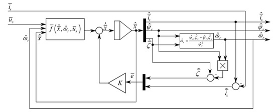
Figure 1.
Block diagram of the extended speed observer.
4. Dynamics of the Extended Speed Observer
The stability of the observer is assured by proper placement of the poles of the linearized observer. Equations of the dynamics of errors of the observer are formed by substituting Equations of the model (6) from the first two equations of the observer (10). The third Equation from (10) that describes dynamics of the additional variable remains unchanged as it is impossible to express estimated rotor speed or rotor speed estimation error with defined in (13). The equations describing dynamics of the observer errors have the following form:
where:
The linearized system (18) has the form of (21), where x and u are state variable and input vectors respectively, * denotes values in an operating point and Δx is the vector of deviations from the operating point:
It is expected that in a steady state, the observer estimates variables with no errors. Therefore, the operating point asserts zero estimation error. This goal is achieved when the estimated ζ satisfies (5). The operating point and vector of deviations from the operating point are defined as follows:
A state matrix of the linearized system is presented in (26). The coefficients of the terms of the linearized system depend on constant values, like observer gains, and on variables, like compounds of the stator current or rotor flux vectors. As those compounds change sinusoidally in a stationary reference frame, it is impossible to perform analysis of placement of the poles. For this reason, the system (18) has been transformed to the rotor flux reference frame where d, q compounds of the rotor flux vector meet the following conditions:
The compounds of vectors in such a reference frame are constant in a steady state. This transformation ensures constant values of elements of the state matrix and enables analysis of placement of the poles.
According to Lyapunov’s first method, all poles of a linearized system must be placed in the left half of the s-plane (poles need to have a negative real part) to maintain stability. Elements of the state matrix (26) depend on:
- Coefficients a1–a6 that depend on machines parameters (resistances and inductances);
- Observer gains k11–k34;
- Real values of the rotor speed and the compounds of the stator current and rotor flux vectors.
As can be seen above, the dynamic properties of the observer depend not only on the observer gains but also on the operating point of the machine. In the rotor flux reference frame, compound ψrd is equal to the rotor flux vector module. Stator current compounds in steady state depend on the rotor flux vector module and torque T:
The rotor flux vector module is usually kept at a constant value, close to the nominal value, by the control system, hence it can be treated as constant as well as coefficients a1–a6. Rotor speed and external torque can change in a wide range, therefore during gains selection, it must be taken into account and the conditions of the stability of the observer must be satisfied for all possible values of the rotor speed and load torque.
5. Gains Selection Using a Genetic Algorithm
The dynamic properties of the extended speed observer depend on the gains of the observer. Due to the high dimension number of the state matrix and its lack of symmetry, it is not possible to perform analytical gains selections like in [26]. Usage of metaheuristic optimization algorithms, like genetic algorithms, is proposed instead. The success of gains selection using such techniques depends on proper fitness function definition.
During gains selection, multiple criteria can be considered, like stability or presence of oscillations during transient states of the observer. Such a multiobjective optimization problem can be solved using linear scalarization, where non-negative weights are assigned to each objective function. The goal of the gains selection algorithm is to minimize the following function, that represents quality index:
where n is the number of criteria, w is the vector of weights, λ is the vector of poles of the observer (30) where σλ is the rate of decay and wλ is the frequency of oscillation:
The first objective is to place all poles outside of the restricted zone, in the left half of the s-plane, to ensure stability. The observer, as it is run on a digital signal processor, is part of a discrete system. Therefore, it is important that the rate of decay σλ of the poles is higher than the sampling period as well as the frequency of oscillation ωλ is a few times lower than the sampling frequency. This expands the restricted zone to exclude poles with big imaginary parts as well as with big negative real parts. The objective function related to the restricted zone can be defined as a sum of functions defining permissible real and imaginary parts for each of the poles:
where:
where σmax < σmin and both are negative. The function returns zero if all of the poles are in the allowable area. When the poles deflect from this zone, the returned value of the function rises linearly to facilitate the optimization algorithm in relocating poles out of the restricted zone. Coefficients ar, ars, ai define the slope of those functions. It is suggested that the σmin should be a small negative number, rather than zero, to ensure that poles with small positive real part yield sufficiently high value of the objective function and avoid marginal stability of the observer.
It is expected that the observer’s dynamic is faster than the object’s dynamic. It can be achieved by placing poles of the observer far away on the left side from the imaginary axis. The settling time is determined mainly by poles with the slowest rate of decay (the dominant poles). Therefore, the goal is to place the dominant poles of the observer possibly far from the imaginary axis. The objective function related to this criterion can be defined as the rate of decay (the real part) of the dominant pole:
For a stable observer, the function returns a negative value. Lower values imply a faster observer response.
The last objective, related to the dynamic properties of the observer, is to minimize oscillations in the transient states of the observer. Such oscillations may have a negative impact on the control system of the electric drive. A minimal value of the damping ratio of ξmin = 0.707 is assumed. A damping ratio for a pair of poles is defined as:
The condition of the proposed minimal damping ratio is fulfilled if the distance of a pair of poles from the imaginary axis is greater or equal to the distance from the real axis. An objective function related to the damping ratio condition has the following form:
where:
where r is a real part of the dominant poles.
Function f3 returns 0 if sufficient dumping is ensured and a positive value otherwise. Function f3a returns zero if the distance of the pole to the imaginary axis is equal to the distance to the real axis (in that case the damping ratio is equal to ξ = 0.707) and rises linearly with decreasing damping ratio. The function returns 1 for a damping ratio equal to zero.
In the case of the analyzed observer, up to three pairs of conjugate poles can be present. Oscillations related to the poles placed far on the left side of the s-plane have less impact on the transient states of the observer than the damping ratio of the dominant poles. Therefore, function f3b has been introduced as a weighting factor which is equal to 1 for dominant poles and exponentially falls to zero with a distance of the pair of poles from the dominant poles.
Measurement errors of known state variables can lead to estimation errors. High observer gains may amplify those errors, therefore, objective function f4 has been introduced in order to minimize the values of the observer gains:
Only gains that amplify stator current errors are subject to function f4 as only those errors are based on the measured values. Variable , defined in (13), depends only on estimated variables, therefore the remaining gains are not taken into account during gains minimization.
The form of fitness function (29) allows us to include all of the presented objectives with specific weights. It is suggested to assign a significantly higher value to w1 (weight related to objective of stability) than to other weights. In that case, for an unstable solution, the terms of the fitness function related to the other objectives have negligibly low values and the priority is to satisfy stability conditions first. When all of the poles are out of the restricted areas on the complex plane, function f1 returns 0. The gains are then tuned to minimize other objective functions.
Observer gains are real numbers; therefore, a real coded genetic algorithm has been used in gains selection where a chromosome is represented by a vector of 12 gains. A tournament selection is used, where the best individual from randomly chosen candidates is moved into the mating pool. Offspring is created from individuals from the mating pool using a whole arithmetic crossover:
where Ka and Kb are parents from the mating pool, α~U(0,1) and U is a uniform random function. New individuals may be subject to mutation algorithm. A non-uniform mutation method is used:
where α is a random value between 0 and 1, kmut is mutated observer gain, k is the original value and kmin, kmax are minimal and maximal values of the observer gains. Function Δ(g):
for β~U(0,1), returns a random value between 0 and 1 for the initial generation but with increasing generation g its upper bound decreases to zero in the final generation gmax. Therefore, the impact of mutation is lower in older generations. Larger values of coefficient b result in quicker annealing.
6. Gains selection results
In the following studies, an induction machine, whose parameters are presented in Appendix A, is considered. During gains selection, nominal values of the rotor speed, the rotor flux module and torque are assumed. Figure 2 presents the fitness function value of the best individual in a function of generation in 10 consecutive gains selection attempts for genetic algorithm and fitness function parameters presented in Appendix B.
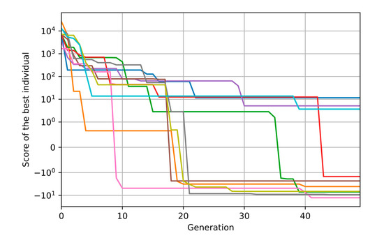
Figure 2.
Fitness function values of the best individual in the function of generation for 10 consecutive gains selection attempts.
Negative fitness value means that all of the poles are placed in an acceptable area and the observer is stable, whereas large positive values indicate lack of stability. As can be seen in Figure 2 all individuals in the first generation yield positive fitness values greater than 1000. This means that none of the few thousand randomly chosen gain sets guarantee the stability of the observer. However, in all attempts of gains selection using the genetic algorithms, fitness value reached acceptable values in the last generation, proving that heuristic methods can be successfully used to find solutions in such a complex, multidimensional problem.
As was mentioned in Section 4, placement of the poles of the observer depends on the machine parameters, observer gains and the operating point of the machine understood as the rotor speed, module of the rotor flux and torque. Machine resistances and inductances do not vary significantly and are assumed to be constant for the purpose of this paper. The only parameters of the state matrix (26) that can change in a wide range are the rotor speed, the rotor flux and torque. This means that the dynamic properties, including stability of the observer, depend on those variables. As the fitness function describes the dynamic properties of the observer at a given operating point of the machine, the impact of changes on the operating point of the machine must be investigated. Such a study has been performed for a constant gains set, defined in Appendix C, which was selected using the proposed algorithm for nominal values of the rotor speed, rotor flux module and torque.
The influence of rotor flux module on the placement of the poles of the observer has been presented in Figure 3. The study has been performed for nominal rotor speed and load torque T = 0.35 (roughly half of the nominal torque). As can be seen from the figure, poles remain almost constant, therefore changes of the rotor flux module do not affect the observer dynamic properties.
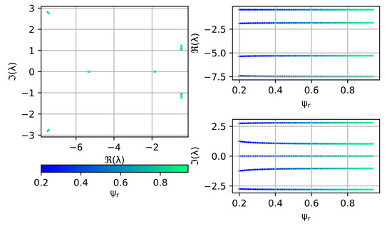
Figure 3.
Poles placement of the observer in the function of the rotor flux module under nominal rotor speed and torque T = 0.35.
Rotor flux is usually kept at a constant, close to nominal, value by a control system. It is possible though to lower the rotor flux when the machine is not operating at full load in order to reduce the core losses. The investigated observer can be used without any gains adjustment in such conditions.
Figure 4 presents the impact of torque changes on the placement of the poles of the observer. The analysis has been performed under nominal rotor speed and rotor flux. In this case, positive values of the torque mean that the machine is operating as a motor and negative values denote operation as a generator. The figure shows that poles of the observer are not affected by changes of the load of the machine regardless of the operation mode. Therefore, the same set of observer gains can be used at the whole range of torque values.
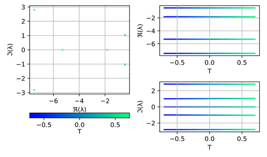
Figure 4.
Poles placement of the observer in the function of the load torque under nominal rotor speed and nominal rotor flux.
As can be seen in Figure 5, rotor speed has a significant influence on the dynamics of the observer. With lower speed, dominant poles of the observer move closer to the imaginary axis. Gains selection, in this case, has been performed for the nominal speed, therefore poles are indeed placed in an allowable area for this operating point. For small speeds though, dominant poles may even cross the imaginary axis leading to instability of the observer. It is also worth noting that the analyzed extended observer has different dynamic properties after changing the rotation direction. In this case, the observer is not stable for negative values of the rotor speed.
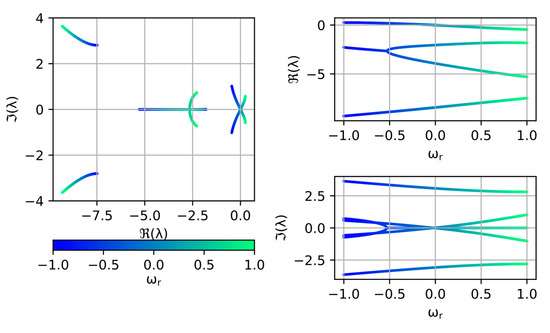
Figure 5.
Poles placement of the observer in the function of the rotor speed under nominal rotor flux module and no load.
To explain and possibly find a solution to observer properties asymmetry after rotation direction change, the extended induction machine model symmetry is analyzed first. Vectors presented in the first equation of the extended induction machine model (6) are shown in Figure 6. If the machine is operating as a motor, stator current vector precedes rotor flux vector. In the case of positive rotation speed (all vectors rotate counterclockwise), vector ζ coincides with the rotor flux, as by definition (5) ζ is formed by multiplying rotor flux vector by a scalar rotor speed. Multiplication of a vector by imaginary number j rotates the vector by +90 degrees, therefore vector jζ precedes rotor flux vector by 90 degrees. In the case of a negative speed (all vectors rotate clockwise), vector ζ is formed by multiplying rotor flux vector by a negative value, hence it has the opposite direction to the rotor flux vector. Rotated vector ζ (jζ) again precedes the rotor flux vector by 90 degrees. Terms on the right side of the first equation of the extended induction machine model are formed by multiplying black vectors presented in the figure by a constant value that only scales the length of the vector. The greyed-out, not rotated vector ζ is not present in this equation. As can be seen, angles between all the vectors present in the mathematical model remain the same under the same operating conditions regardless of the rotation direction. Similar conclusions can be drawn from analyzing the remaining two equations of the machine. Therefore, it is possible for the extended induction machine model to preserve its properties after a rotation direction change.
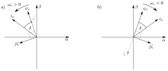
Figure 6.
State variables from the right side of the first equation of the extended induction machine model presented as rotating vectors for: (a) positive speed values (vectors rotating counterclockwise) and (b) negative speed values (vectors rotating clockwise).
Observer equations are based on the object’s mathematical model with the addition of corrective feedback. Estimation errors vectors have been presented in Figure 7. Stator current estimation error is the difference between estimated and real stator current vectors. Corrective feedback related to ζ errors is defined by (5). Assuming symmetric properties of the observer after rotation direction change, vectors of real and estimated stator current and rotor flux for negative speed values (Figure 7b) are symmetric about the axis β to those vectors in case of positive speed (Figure 7a). Due to multiplication by a negative number, vectors and are symmetric (as stator current and rotor flux vectors) and additionally rotated by 180 degrees in case of negative speed values.
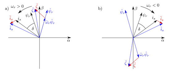
Figure 7.
Real vectors of the state variables of the machine (black), estimated vectors (blue) and estimation errors (red) for: (a) positive speed values (vectors rotating counterclockwise) and (b) negative speed values (vectors rotating clockwise).
Estimated vectors (blue) and error vectors (red) present in the first equation of the observer (10) are shown in Figure 8. Error vectors from Figure 7 are multiplied by observer gains, that affect only the amplitude of the vector, and by imaginary number j, that rotates the vector by 90 degrees. As can be seen in the figure, after rotation direction change, angles between vectors do not remain the same, which can justify the lack of symmetry of dynamic properties of the observer shown in Figure 5.
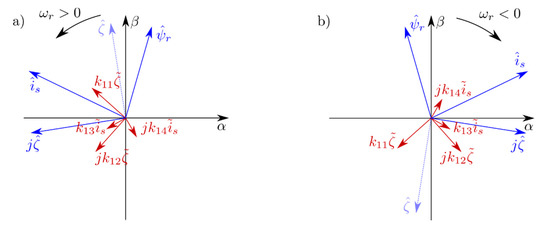
Figure 8.
Vectors from the right side of the first equation of the observer for: (a) positive speed values (vectors rotating counterclockwise) and (b) negative speed values (vectors rotating clockwise).
Vectors that are out of order after direction change are and . Rotating those vectors by 180 degrees, by multiplying gains k11 and k14 by -1 for negative rotation speed values, restores angles between vectors as is shown in Figure 9. By changing the sign of appropriate observer gains after rotation direction change, it may be possible for the observer properties to remain in symmetry.
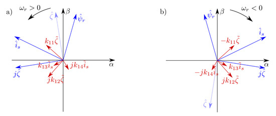
Figure 9.
Vectors from the right side of the first equation of the observer for: (a) positive speed values (vectors rotating counterclockwise) and (b) negative speed values (vectors rotating clockwise) with modified observer gains.
By performing a similar analysis on the other two equations of the observer, it can be concluded that gains k21, k24, k32, k33 also need to change the sign for negative rotation speed values. Therefore, for the observer gains set K+ selected for positive speed values:
the following gains set should be used for negative rotation speed:
Placement of the poles in the function of rotation speed, using the method of gains adjustment after rotation direction change presented above, has been shown in Figure 10. As can be seen, the extended speed observer has now the same dynamic properties regardless of the rotation direction.
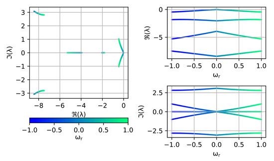
Figure 10.
Poles placement of the observer in the function of the rotor speed under nominal rotor flux module and no load with modified gains after a rotation direction change.
7. Simulation Results
Simulation and experimental studies have been performed on a machine described in Appendix A. Conclusions concerning the dynamic properties of the observer can be drawn by analyzing its impulse response. In a steady state of the machine and the observer, an estimation error of the rotor flux module equal to 0.2 is imposed. Simulation and experimental results, as well as poles placement of the observer for different rotor speed values, have been presented in Figure 11. As it was noted in the previous chapter, rotor speed has a noticeable impact on the dynamics of the observer. For comparison, settling time values estimated from poles placement and measured from simulation results have been presented in Table 1. Settling time estimated from poles placement is calculated based on the time constant of the dominant poles:
where σ is the real part of the dominant pole, T is the time constant of the dominant pole and tsettling is the estimated settling time of the observer.
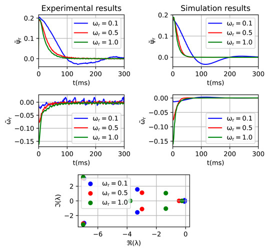
Figure 11.
Experimental and simulation studies of the influence of the rotor speed on the poles placement and impulse response of the observer at nominal load torque and rotor flux.

Table 1.
Comparison of settling time estimated from the placement of the dominant poles with real settling time from simulations.
As can be seen, dynamic properties read from the placement of the poles reflect results acquired from the experiments. In simulations, rotor flux estimation error is a difference between the estimated value and real value. As there is no flux measurement, in real experiments, the rotor flux estimation error is understood as a difference between the estimated rotor flux module and estimated rotor flux module in a steady-state (constant value) of the observer.
The results of the study of the influence of load torque and the rotor flux module on the dynamics of the observer have been shown in Figure 12 and Figure 13. As it was noted before, those two variables have a minor impact on the placement of the poles, therefore, they do not influence the dynamics of the observer, as has been confirmed in the experimental results. Settling time of the impulse response of the observer remains almost the same regardless whether the machine is operating as a generator or as a motor or with a lower rotor flux module.
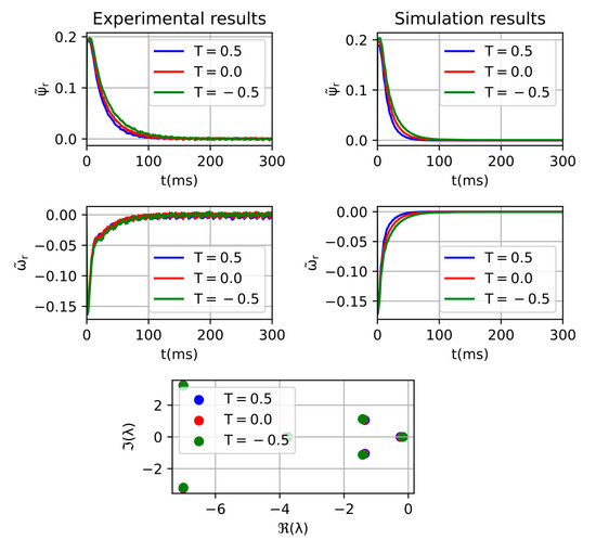
Figure 12.
Experimental and simulation studies of the influence of the load torque on the poles placement and impulse response of the observer at nominal rotor speed and rotor flux.
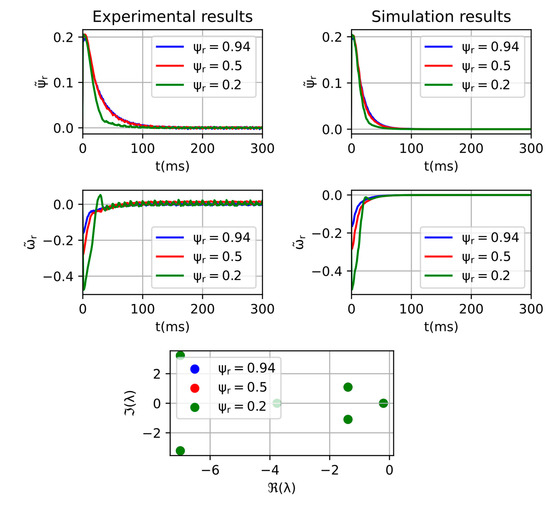
Figure 13.
Experimental and simulation studies of the influence of the rotor flux on the poles placement and impulse response of the observer at nominal rotor speed and no load.
The above experiments have been performed in an open-loop system to eliminate the impact of the control system on the results. Results of the experiments during the reverse of the machine have been presented in Figure 14. Estimated rotor flux is not maintained at a constant level due to usage of a simple open-loop control system, where at very low-speed maintaining constant ratio of voltage module to frequency is not sufficient to provide constant rotor flux.
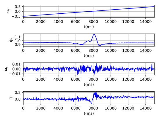
Figure 14.
Experimental results during rotor direction change using the open-loop control system.
Experimental results in a closed-loop sensorless system introduced in [29] have been presented in Figure 15 (slow reverse) and Figure 16 (fast reverse). As can be seen, the observer can be implemented in advanced control systems and cope well with fast dynamic changes of the rotor speed as well as low dynamics of the machine even at a low speed. In the case of fast reverse in the first half of the experiment, the rotor of the machine is being slowed down recovering the energy, therefore it works as a generator, while in the second part when the rotor speed is greater than zero, the machine operates as a motor. Such a transition is still handled well by the observer.
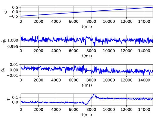
Figure 15.
Experimental results during rotor direction change using the closed-loop control system.

Figure 16.
Experimental results during fast rotor direction change using the closed-loop control system.
8. Discussion and Conclusions
Speed observer based on the extended model of an induction machine requires a selection of 12 gains. Using genetic algorithms with the proposed fitness function provides gains that ensure stability and proper dynamic properties of the observer. This approach also allows setting bands of gains, limiting their values. High gains values of the observer may lead to amplification of measurement errors and have an adverse impact on the quality of estimation. Limiting observer gains may be beneficial in case of noisy current measurements.
A significant drawback of usage of heuristic optimization methods, like genetic algorithms, is a high count of fitness function calls. One of the approaches of evaluation of estimation quality is to perform a simulation and measure quality indices (e.g., settling time, overshot). Fitness function based on simulation is computationally heavy, therefore a quality index based on the placement of poles has been proposed instead. This approach allows the determination of the dynamic properties of the observer without performing a simulation. This significantly reduces the time needed to run the algorithm. Placement of the poles is obtained from linearized equations of the dynamics of the observer, hence conclusions drawn from analysis of the poles are only approximations. Therefore, the final gains set needs to be tested during simulations before it is considered valid and can be used on a real machine.
Comparison of dynamic properties deduced from placement of the poles of the linearized system and real dynamics of the observer has been presented. It is possible to successfully predict the settling time and presence of oscillations based on the distance of the dominant poles from real or imaginary axes. As linearization has been performed about an operating point that provides zero estimation errors, the accuracy of conclusions drawn from the placement of the poles depends on estimation errors. Forcing flux estimation error equal to 0.2 (about 20% of nominal flux) still allows the accurate prediction of dynamic properties of the observer from the placement of the poles.
Analysis of the impact of the operating point of the machine on the placement of the poles shows that the dynamics of the observer are independent of the rotor flux module and torque changes. On the other hand, rotor speed changes have a significant impact on dynamic properties of the observer, causing the estimation errors to decay slower at low speed. There is also a high probability that the observer will lose stability after rotation direction change while using the same observer gains. For that reason, specific gains need to change the sign to persevere dynamic properties. Simulation and experimental studies confirm that the proposed method of gains correction after rotation direction change is valid.
Gains acquired through the proposed method have also been tested during dynamic states of the machine. The observer has been successfully used as feedback of a closed-loop control system to control rotor speed and rotor flux. Estimates are correct for the machine operating as a motor as well as a generator during slow speed changes as well as during fast transitions.
Funding
This research received no external funding.
Conflicts of Interest
The authors declare no conflict of interest.
Appendix A. Induction Machine Parameters
Table A1.
Parameters of the induction machine.
Table A1.
Parameters of the induction machine.
| Quantity | Symbol | Value |
|---|---|---|
| Nominal power | Pn | 5.5 kW |
| Nominal stator voltage | Un | 400 V |
| Nominal stator current | In | 11 A |
| Nominal rotor speed | nn | 1450 rpm |
| Nominal frequency | fn | 50 Hz |
| Stator resistance | Rs | 0.04870 p.u. |
| Rotor resistance | Rr | 0.02613 p.u. |
| Magnetizing inductance | Lm | 2.135 p.u. |
| Stator inductance | Ls | 2.224 p.u. |
| Rotor inductance | Lr | 2.224 p.u. |
Appendix B. Parameters of Genetic Algorithm and Fitness Function
Table A2.
Parameters of genetic algorithm.
Table A2.
Parameters of genetic algorithm.
| Parameter | Value |
|---|---|
| Population size | 500 |
| Max. number of generations gmax | 50 |
| Crossover probability | 0.5 |
| Mutation probability | 0.2 |
| Min. gains value kmin | −10 |
| Max. gains value kmax | 10 |
Table A3.
Parameters of the fitness function.
Table A3.
Parameters of the fitness function.
| Parameter | Value |
|---|---|
| σmax | −12 |
| σmin | −0.001 |
| ωmax | 12 |
| ar | 10 |
| ars | 1000 |
| ai | 10 |
| a | 1 |
Appendix C. Gains of the Observer
Table A4.
Gains of the observer for studies presented in Section 6.
Table A4.
Gains of the observer for studies presented in Section 6.
| Gain | Value |
|---|---|
| k11 | 6.009328 |
| k12 | 1.454451 |
| k13 | −7.339396 |
| k14 | 0.138127 |
| k21 | 0.162761 |
| k22 | 0.047938 |
| k23 | 1.380530 |
| k24 | −0.393255 |
| k3 | −6.946626 |
| k32 | 4.227242 |
| k33 | 1.442308 |
| k34 | −2.179116 |
Table A5.
Gains of the observer for ωr > 0.
Table A5.
Gains of the observer for ωr > 0.
| Gain | Value |
|---|---|
| k11 | −3.195624 |
| k12 | 2.652105 |
| k13 | −6.220342 |
| k14 | 0.723027 |
| k21 | 0.132168 |
| k22 | −0.440498 |
| k23 | −0.351436 |
| k24 | −0.364211 |
| k3 | −5.841087 |
| k32 | −1.939082 |
| k33 | −0.809362 |
| k34 | −1.498938 |
Table A6.
Gains of the observer for ωr < 0.
Table A6.
Gains of the observer for ωr < 0.
| Gain | Value |
|---|---|
| k11 | 3.195624 |
| k12 | 2.652105 |
| k13 | −6.220342 |
| k14 | −0.723027 |
| k21 | −0.132168 |
| k22 | −0.440498 |
| k23 | −0.351436 |
| k24 | 0.364211 |
| k3 | −5.841087 |
| k32 | 1.939082 |
| k33 | 0.809362 |
| k34 | −1.498938 |
References
- Ryndzionek, R.; Michna, M.; Ronkowski, M.; Rouchon, J.F. Chosen Analysis Results of the Prototype Multicell Piezoelectric Motor. IEEE/ASME Trans. Mechatron. 2018, 23, 2178–2185. [Google Scholar] [CrossRef]
- Ryndzionek, R.; Sienkiewicz, Ł.; Michna, M.; Kutt, F. Design and Experiments of a Piezoelectric Motor Using Three Rotating Mode Actuators. Sensors 2019, 19, 5184. [Google Scholar] [CrossRef] [PubMed]
- Morawiec, M. Sensorless Control of Induction Machine Supplied by Current Source Inverter. Asian J. Control 2015, 17, 2403–2408. [Google Scholar] [CrossRef]
- Finch, J.W.; Giaouris, D. Controlled AC electrical drives. IEEE Trans. Ind. Electron. 2008, 55, 481–491. [Google Scholar] [CrossRef]
- Pacas, M. Advanced Control Schemes. IEEE Ind. Electron. Mag. 2011, 5, 16–23. [Google Scholar] [CrossRef]
- Blecharz, K.; Morawiec, M. Nonlinear Control of a Doubly Fed Generator Supplied by a Current Source Inverter. Energies 2019, 12, 2235. [Google Scholar] [CrossRef]
- Benlaloui, I.; Drid, S.; Chrifi-Alaoui, L.; Ouriagli, M. Implementation of a new MRAS speed sensorless vector control of induction machine. IEEE Trans. Energy Convers. 2015, 30, 588–595. [Google Scholar] [CrossRef]
- Korzonek, M.; Tarchala, G.; Orlowska-Kowalska, T. A review on MRAS-type speed estimators for reliable and efficient induction motor drives. ISA Trans. 2019, 93, 1–13. [Google Scholar] [CrossRef] [PubMed]
- Niestroj, R.; Bialon, T.; Pasko, M.; Lewicki, A. Selected dynamic properties of adaptive proportional observer of induction motor state variables. In Proceedings of the 2016 Selected Issues of Electrical Engineering and Electronics WZEE, Rzeszow, Poland, 4–8 May 2016. [Google Scholar]
- Bialon, T.; Niestroj, R.; Pasko, M.; Lewicki, A. Gains selection of non-proportional observers of an induction motor with dyadic methods. In Proceedings of the 2016 13th Selected Issues of Electrical Engineering and Electronics (WZEE), Rzeszow, Poland, 4–8 May 2016. [Google Scholar]
- Niestroj, R.; Bialon, T.; Pasko, M.; Michalak, J. Study of adaptive proportional observer of state variables of induction motor taking into consideration the generation mode. In Proceedings of the 2017 International Symposium on Electrical Machines SME, Naleczow, Poland, 18–21 June 2017. [Google Scholar]
- Benchaib, A.; Rachid, A.; Audrezet, E.; Tadjine, M. Real-time sliding-mode observer and control of an induction motor. IEEE Trans. Ind. Electron. 1999, 46, 128–138. [Google Scholar] [CrossRef]
- Zhao, L.; Huang, J.; Liu, H.; Li, B.; Kong, W. Second-order sliding-mode observer with online parameter identification for sensorless induction motor drives. IEEE Trans. Ind. Electron. 2014, 61, 5280–5289. [Google Scholar] [CrossRef]
- Maiti, S.; Verma, V.; Chakraborty, C.; Hori, Y. An adaptive speed sensorless induction motor drive with artificial neural network for stability enhancement. IEEE Trans. Ind. Inform. 2012, 8, 757–766. [Google Scholar] [CrossRef]
- Li, Y.; Pu, Y. Application of fuzzy neural network in the speed control system of induction motor. In Proceedings of the 2011 IEEE International Conference on Computer Science and Automation Engineering, Shanghai, China, 10–12 June 2011; pp. 673–677. [Google Scholar] [CrossRef]
- Iqbal, A.; Rizwan Khan, M. Sensorless control of a vector controlled three-phase induction motor drive using artificial neural network. In Proceedings of the 2010 Joint International Conference on Power Electronics, Drives and Energy Systems & 2010 Power India, New Delhi, India, 20–23 December 2010. [Google Scholar] [CrossRef]
- Khan, M.R.; Iqbal, A. Extended Kalman filter based speeds estimation of series-connected five-phase two-motor drive system. Simul. Model. Prac. Theory 2009, 17, 1346–1360. [Google Scholar] [CrossRef]
- Djellouli, T.; Moulahoum, S.; Boucherit, M.S.; Kabache, N. Speed & flux estimation by extended Kalman filter for sensorless direct torque control of saturated induction machine. In Proceedings of the 2011 International Siberian Conference on Control and Communications (SIBCON), Krasnoyarsk, Russia, 15–16 September 2011; pp. 23–26. [Google Scholar] [CrossRef]
- Laatra, Y.; Lotfi, H.; Abdelhani, B. Speed sensorless vector control of induction machine with Luenberger observer and Kalman filter. In Proceedings of the 2017 4th International Conference on Control, Decision and Information Technologies (CoDIT), Barcelona, Spain, 5–7 April 2017; pp. 714–720. [Google Scholar] [CrossRef]
- Morawiec, M.; Blecharz, K.; Lewicki, A. Sensorless rotor position estimation of doubly fed induction generator based on backstepping technique. IEEE Trans. Ind. Electron. 2020, 67, 5889–5899. [Google Scholar] [CrossRef]
- Morawiec, M.; Lewicki, A. Application of Sliding Switching Functions in Backstepping Based Speed Observer of Induction Machine. IEEE Trans. Ind. Electron. 2020, 67, 5843–5853. [Google Scholar] [CrossRef]
- Krzeminski, Z. A new speed observer for control system of induction motor. In Proceedings of the IEEE 1999 International Conference on Power Electronics and Drive Systems, Hong Kong, China, 27–29 July 1999; pp. 555–560. [Google Scholar] [CrossRef]
- Krzemiński, Z. Observer of induction motor speed based on exact disturbance model. In Proceedings of the 2008 13th International Power Electronics and Motion Control Conference, Poznan, Poland, 1–3 September 2008; pp. 2294–2299. [Google Scholar] [CrossRef]
- Yongchang, Z.; Zhengming, Z.; Ting, L.; Liqiang, Y.; Wei, X.; Jianguo, Z. A comparative study of Luenberger observer, sliding mode observer and extended Kalman filter for sensorless vector control of induction motor drives. In Proceedings of the 2009 IEEE Energy Conversion Congress and Exposition, San Jose, CA, USA, 20–24 September 2009; pp. 2466–2473. [Google Scholar]
- Weiwen, W.; Zhiqiang, G. A comparison study of advanced state observer design techniques. In Proceedings of the 2003 American Control Conference, Denver, CO, USA, 4–6 June 2003; pp. 4754–4759. [Google Scholar]
- Białoń, T.; Lewicki, A.; Pasko, M.; Niestrój, R. Non-proportional full-order Luenberger observers of induction motors. Arch. Electr. Eng. 2018, 67, 925–937. [Google Scholar] [CrossRef]
- Alanis, A.Y.; Arana-Daniel, N.; Lopez-Franco, C.; Sanchez, E.N. PSO-gain selection to improve a discrete-time second order sliding mode controller. In Proceedings of the 2013 IEEE Congress on Evolutionary Computation, Cancun, Mexico, 20–23 June 2013; pp. 971–975. [Google Scholar] [CrossRef]
- Bhangu, B.S.; Bingham, C.M. GA-tuning of nonlinear observers for sensorless control of automotive power steering IPMSMs. In Proceedings of the 2005 IEEE Vehicle Power and Propulsion Conference, Chicago, IL, USA, 7 September 2005; pp. 772–779. [Google Scholar] [CrossRef]
- Krzemiński, Z. Nonlinear Control of Induction Motor. In Proceedings of the 10th Triennial IFAC Congress on Automatic Control, Munich, Germany, 27–31 July 1987; Volume 20, pp. 357–362. [Google Scholar]
© 2020 by the author. Licensee MDPI, Basel, Switzerland. This article is an open access article distributed under the terms and conditions of the Creative Commons Attribution (CC BY) license (http://creativecommons.org/licenses/by/4.0/).