Abstract
The efficient spatial load forecasting (SLF) is of high interest for the planning of power distribution networks, mainly in areas with high rates of urbanization. The ever-present spatial error of SLF arises the need for probabilistic assessment of the long-term point forecasts. This paper introduces a probabilistic SLF framework with prediction intervals, which is based on a hierarchical trending method. More specifically, the proposed hierarchical trending method predicts the magnitude of future electric loads, while the planners’ knowledge is used to improve the allocation of future electric loads, as well as to define the year of introduction of new loads. Subsequently, the spatial error is calculated by means of root-mean-squared error along the service territory, based on which the construction of the prediction intervals of the probabilistic forecasting part takes place. The proposed probabilistic SLF is introduced to serve as a decision-making tool for regional planners and distribution network operators. The proposed method is tested on a real-world distribution network located in the region of Attica, Athens, Greece. The findings prove that the proposed method shows high spatial accuracy and reduces the spatial error compared to a business-as-usual approach.
1. Introduction
1.1. Motivation
Load forecasting was always a topic of high priority for the distribution network operators (DNOs). Planning purposes have revealed the need for efficient load forecasting tools that cover the load growth for a time horizon from eight to twenty years [1]. In the late 1980s, the ever-increasing operational challenges leaded the electrical engineers to develop tools to predict the load variance in time windows up to one day. According to [2], load forecasting can be roughly divided in two main categories depending on the time horizon of forecasting: (a) short-term load forecasting (STLF) that mainly refers to time periods spanning from one day up to a few days and is dedicated for the operational planning of the distribution networks, and (b) long-term load forecasting (LTLF) that refers to time periods longer than three years and is necessary for network planning, expansion and maintenance.
For instance, in [3], the decisions made for sizing and allocation of distributed generation units depend on the load growth in the service area of the distribution network. The method of [4] considers the uncertainties of long-term load to optimize multiple planning alternatives (reinforcement of substations and distribution lines, addition of new lines, and placement of capacitors). The review work [5] highlights the importance of distribution systems planning in satisfying the rate of load growth. In [6], a novel method is proposed for multistage coordinated planning in active distribution networks considering high penetration of renewables and load scenarios based on LTLF.
In recent years, and particularly in cities that are characterized by increased urban development, LTLF is getting more and more crucial for the network planners and reveals the need for more granular spatial forecasting. As defined in [1,7], spatial load forecasting (SLF) is a process of LTLF that geographically allocates the future electric loads to the service territory of a distribution network, i.e., a wider area (e.g., village, neighborhood, municipality, or city) that is supplied by one or more high voltage (HV)/medium voltage (MV) substations, which consequently supply several MV/low voltage (LV) distribution substations. With SLF, the magnitude of future loads (mainly the forecasted peak demand) is allocated to the small areas or the distribution equipment (distribution transformers and LV feeders) of a distribution network’s service territory [1,2,7]. The latest developments and trends in SLF are summarized by the authors of [8] to highlight the emerging role of SLF in planning of transmission and distribution networks. SLF in distribution networks is mainly driven by land use change, whereas SLF in transmission planning uses the economic growth as the basic driver [9].
1.2. Bibliography Review
Several methods have been proposed in the bibliography to forecast the electric load growth on a spatial basis. In all of these methods, the service territory is divided into adequate number of smaller areas to better accomplish the geographic location of load growth [7]. Most of the methods give priority in forecasting the load growth of the service territory based on conventional prediction methods, and then determine the evolution of land use to allocate the expected load increase. The load growth is not only driven by land use change, but also depends on the integration of new technologies of distributed energy resources (DERs), such as electric vehicles (EVs) charging and electric heat pumps (EHPs), as well as the implementation of energy efficiency programs. However, high levels of uncertainty are introduced in the spatiotemporal allocation of future loads, as the future land use, the urban development and the allocation of DERs depend on various geographical, social and economic factors.
The SLF methods are generally divided into two main categories as follows:
- Simulation methods: these methods are based on modeling the load growth process to reproduce the load history in order to determine the year, location, and magnitude of future loads in the service territory. The simulation methods give satisfactory results in cases of high spatial analysis of the service territory, and in cases of long-term forecasting. Their structure is usually based on artificial intelligence methods and machine learning approaches, such as cellular automata theory, multi-agent systems, evolutionary and heuristic algorithms. Though, simulation methods require a lot of training data, well-organized in databases, and the contribution of human knowledge (experienced engineers or experts in urban development).
- Trend methods: Unlike simulation methods, trend methods are based on historical data of annual peak load and extrapolate a time-series to the future by fitting the past load pattern to a suitable function. It is often necessary to calculate the horizon year load (HYL), i.e., the load of fully saturated small areas. The HYL improves the fitting accuracy of data to the historical load curve of a small area [7]. In general, trend methods give satisfactory results in case of low spatial analysis of the service territory and in cases of short-term forecasting. The fitting function is usually applied by using linear or polynomial regression. Some of the advantages of trend methods include simplicity and ease of use.
Determining future land use is the most important process of SLF and belongs to the category of simulation methods. The research works that have been proposed in this field simulate the evolution of land use on a grid resolution basis, i.e., the service territory of the distribution network is divided into small areas (or sub-regions) and each of them represents a group of consumers along with their aggregated load. In [10], a simple, but efficient, methodology to forecast the future land use is proposed by taking advantage of concepts such as knowledge extraction algorithms and evolutionary algorithms, while also considering the accidental settlement of new consumers in the service area. In [11], the authors of [10] expand their work by proposing a novel method that exploits the concept of cellular automata. The service territory is divided in small areas, called as cells. Each cell is characterized by a discrete state, which changes according to the cell’s current state and the interaction with its neighborhood. In [12], the changes in land use are simulated by employing the concept of cellular automata, and consequently the Markov model is applied to improve the forecasting procedure. In [13], the theory of cellular automata is employed once more to forecast and allocate the future loads, while the authors utilize the available geographical information systems (GIS) technology and also consider the risk factors (natural environment, land-use management, economic development, population, and urban policies) that are always in presence. The problem of SLF is approached with multi-agent systems by the authors of [14,15]; a method that is similarly used by researchers in other fields, such as urban planning. The findings of [14,15] show that the spatial error remains low when compared with real data even in cases of few initial data. All of the methods proposed in [10,11,12,13,14,15] use artificial intelligence approaches, and their common advantages are: (a) few raw data of spatial information, (b) no need for calculation of the S-curves that represent the load growth in every small area, and (c) simple mathematical formulas that lead to low computational effort.
The second main category of SLF refers to trend methods, which adjust the available historical load data to a suitable curve. Gompertz curve, the well-known S-curve, is the curve that represents the load growth in a small area or a sub-region. In [16], the developed methodology adjusts the historical load data and constructs the S-curves of the small areas of the service territory. The forecasted load of the service territory is firstly allocated to the occupied small areas according to their S-curves, and subsequently the remaining load is allocated to the non-occupied small areas, with those ones having the highest development score being in priority. A SLF tool is developed in [17], based on S-curves of small areas, historical load data and land use. The magnitude of peak load is forecasted with extrapolation, while the future land use is determined with a simulation algorithm. In [18], a human-machine method that uses data of land use and the planners’ knowledge is introduced to calculate the HYL. The HYL denotes the load of fully saturated small areas, or in other words it gives an estimation of the farthest forecasting year’s load, as mentioned in [18].
Other research works, which are related to SLF and cannot be categorized in one of the two aforementioned main categories, are [19,20,21]. In [19], a trade-off between accuracy and computational time is investigated by calculating the average absolute error of SLF in the service territory for different values of spatial resolution. In [20], the preferences of consumers that affect the creation of new loads in the service territory are given within a map, which in fact provides the likelihood of development of each small area; the proposed method is based on statistical analysis and it is distinguished for ease of use and implementation in statistical analysis software. Τhe work [21] adopts the principles of fractal geometry to simulate the load growth in a grid-based model. The power-law distribution of fractal exponent is used for the proposed SLF method of [21].
Recent developments in metering infrastructure and databases have provided electric utilities with a significant amount of highly granular data, both temporally and spatially [2]. The high research interest in the field of forecasting techniques, as well as the available data of higher granularity, have converted spatial load forecasting into hierarchical load forecasting, which in turn can cover forecasting at various levels, from the household level to the corporate level [22]. Hierarchical forecasting can be realized by a single top-down allocation of the corporate forecasting or a combined bottom-up aggregation and top-down allocation. In the former, the allocation can be realized according to the geospatial characteristics and the land use of the service territory. In the latter, the bottom-up aggregation takes advantage of the spatial granularity of the historical data of the bottom level to better fit the forecasting of the top level. In any case, the correlation of the forecasting errors at the different levels of the hierarchical procedure should be carefully considered.
Modern SLF methodologies should also take into account the adoption of new technologies that increase the consumption of electricity, such as EVs and EHPs, or contribute to energy savings and peak shaving, such as demand-side flexibility schemes that are proposed in [23]. In [24], a methodology is proposed to quantify the effect of different factors on the adoption of grid-connected residential DERs, i.e., photovoltaics (PVs), EVs and EHPs. The work [25] presents a novel approach that predicts the allocation of DERs, such as PVs and EVs, and assesses the impact of such DERs in the distribution networks. Both [24] and [25] can be incorporated into a method of SLF for planning problems for better understanding the spatiotemporal evolution of loads. In case the adoption of EVs and/or EHPs is considered, underestimation of load forecasting can be avoided. On the other hand, overestimation of load forecasting can be avoided, when SLF considers the energy efficiency programs that are scheduled to be implemented. Given that most of the SLF methods predict the annual peak load, the integration of residential DERs that produce energy during midday, such as PVs, is not crucial.
1.3. Article Contribution
From the above bibliography review in the field of SLF, it is worth noting that none of the works has proposed or introduced a methodology for probabilistic SLF (P-SLF). Although, as mentioned in [26], load forecasting by nature is a stochastic problem, most of the proposed methods for SLF give point forecasts instead of probabilistic forecasts. Probabilistic forecasting is of high interest, especially in cases of decision making, as it integrates the forecasting error in the upcoming load forecasts. In that setting, it depends on the planner’s choice to make decisions based on less or more conservative scenarios. The main contributions of this paper are the following:
- It proposes a novel probabilistic framework for SLF based on a hierarchical trending method that uses the well-known S-curves for fitting the historical load data.
- It introduces the construction of the prediction intervals of the proposed P-SLF by employing the spatial error metric of root-mean-squared error (RMSE) along the service territory.
- The proposed method is applied on a real-world distribution network and its effectiveness is validated by comparing the results obtained to a business-as-usual (BaU) approach.
- The proposed method can serve as a decision making tool for DNOs and city planners, who wish to choose between an ordinary and a more conservative forecasting.
The remainder of this paper is organized as follows: Section 2 analyzes the basic parameters and the input data that are used in the procedure of SLF. Section 3 gives the structure of the SLF procedure and formulates the mathematical model of the proposed method. Section 4 is dedicated to present the error metrics that are employed to evaluate the proposed method. Section 5 presents the case study under examination and discusses the results obtained. Section 6 concludes the paper and proposes future research work.
2. Overview of Spatial Load Forecasting
2.1. Service Territory of Distribution Networks
The service territory of a distribution network is the wider area, in which there are one or more HV/MV substations and consequently several distribution substations (MV/LV substations). The service territory of a distribution network extends to a specific geographical area (e.g., a municipality or a city) and is operated by an electricity distribution company.
In any case, the forecasting of the magnitude and the position of future loads should be carried out with sufficient geospatial analysis to facilitate the planning of the distribution network equipment (sizing and siting) [4]. To achieve that, the service territory is initially divided into a number of sub-regions (small areas), and subsequently the future loads are allocated to those sub-regions. There are two main approaches of dividing the service territory into small areas:
- Small areas of irregular shape. Each small area represents an area that is supplied by an individual distribution substation or a group of distribution substations. Each small area covers an area of varying size (in km2).
- Small areas of square shape. All small areas cover equal size of land (in km2). An individual distribution substation is possible to supply consumers of one or more small areas. The number of small areas is equal to N = n × n, where n is the number of small areas along the width of the service territory. The small areas are usually grouped in a hierarchical procedure to form sub-regions. Thus, there are multiple levels in which the service territory is divided and the sub-regions of the lower levels are grouped to form the sub-regions of the upper level. The small areas belong to the bottom level (level #1). The number of levels depends on the spatial resolution of the bottom level and the small areas, or sub-regions, are gathered in groups of four to create the sub-region of the upper level.
In this paper, the service territory is divided into small square areas of equal size and the hierarchical approach of bottom-up aggregation is applied. This approach is explained in detail in Section 3.
2.2. Spatial Resolution
The selection of spatial resolution of the grid used in SLF is one of the parameters that matters the most. As investigated in [19], high resolution usually leads to more accurate results, but increases the computational time. The spatial resolution varies depending on the application, the planning needs of the distribution network and the type of equipment that is studied to be installed. The granularity of the service territory varies from 0.25 km2 to 2.5 km2 for distribution network planning, according to [8]. Typically, electricity distribution companies use small areas of 0.63 km2 for planning studies of distribution substations and small areas of 0.28 km2 for planning the installation of new LV feeders in the service territory [1,7]. All the works [10,11,14,15] use a grid of square small areas of 0.5 km2 each. In [20], the service territory is covered by a grid of 1024 square small areas of 0.5 km2 each too, whereas the spatial resolution is set to 0.12 km2 for each square small area in [21].
2.3. S-Curve Parameters
The load growth of small areas is directly affected by the number of consumers and the type of consumers located in each small area (i.e., by the type of land use by consumers). In contrast with the load growth of a wider area (e.g., the service territory), which presents a gradual ascending trend, the load growth of small areas is usually modeled with the Gompertz curve, also well-known as S-curve due to its shape [1,2,3,4,5,6,7]. The area is initially vacant (dormant period), until the first loads are installed in the area. Then, the load increase of a small area is achieved within a few years (growth period) and thereafter a saturation period occurs. As depicted in Figure 1, the smaller the area under consideration is, the sharper the S-curve is (larger slope of increase) and the shorter the growth period is.
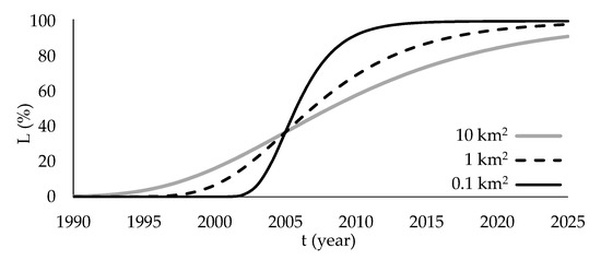
Figure 1.
S-curve shape in relation to the area size [1].
The mathematical formula of S-curve is given by Equation (1). The main parameters that affect the peak load in year t, Lt, are: (a) horizon year load (HYL), (b) ramp-up time (dt), and (c) slope of the ramp (c). Equation (1) holds for HYL greater than zero and for c parameter less than or equal to zero.
2.4. Spatial & Temporal Database
The existence of a spatiotemporal database is a prerequisite for efficiently solving the SLF problem. The spatial database comprises the input data of SLF with regards to the information about consumer categories, historical load data, distribution substations, LV power supply feeders, statistical load curves for each consumer category, and categorization of areas depending on land use. The data provided must be adequate and valid, and shall comprise at least the commercial and technical information that are described hereafter.
2.4.1. Distribution Substation Data
The technical database of the DNO usually contains data relevant to the distribution network’s MV/LV substations. The most important information is the following:
- Geospatial coordinates (longitude and latitude) of the distribution substations.
- Installed capacity of the distribution substations given in kVA (e.g., 400 kVA, 630 kVA).
- Year of installation of the distribution substations.
- Raw data of annual peak load per distribution substation given in kW or kVA (depending on the available type of measurement, i.e., active power or apparent power, respectively). The planners should always consider the relevant power factor, should industrial infrastructure that mainly consumes significant amounts of reactive power is present in the service territory. All data are processed to be used with a common measurement unit. In this paper, the active power, given in kW, at the MV level per distribution substation is considered. In case no measurements are available, the historical load data are sourced from engineers’ estimations.
2.4.2. Small Area Data
The data related to each small area of the service territory are the following:
- Geospatial coordinates of each small area (a representative point is selected, e.g., the center of the square or the upper left corner of the square).
- Current land use per land use type given in percentage (%) or in km2. Some types of the land use are: residential, commercial, industrial, business, transportation, and public sector. The type “vacant” is always in presence and is related to the unoccupied areas, e.g., nature, woodland, sea, and rivers. These data are usually extracted from GIS or from the DNO’s commercial databases.
- Future land use per land use type given in percentage (%) or in km2. These data are usually determined by planners’ knowledge or, more rarely, are calculated by heuristic and evolutionary algorithms.
2.4.3. Neighborhood Data
Each small area is surrounded by other small areas. The small areas are grouped in a suitable manner to form larger sub-regions. In the hierarchical procedure, which is described in Section 3, the presence of a neighborhood table is mandatory for the creation of the sub-regions of the upper levels. The neighborhood table can be easily constructed using the geospatial coordinates of each small area and aggregating them in appropriate groups.
3. Problem Formulation
The proposed methodology followed for SLF is structured by five main modules: (a) normalization module, (b) future land use module, (c) HYL module, (d) hierarchical forecasting module, and (e) probabilistic forecasting module, as depicted in the flowchart of Figure 2. This flowchart also summarizes the methodology and serves as an overview for the reader.
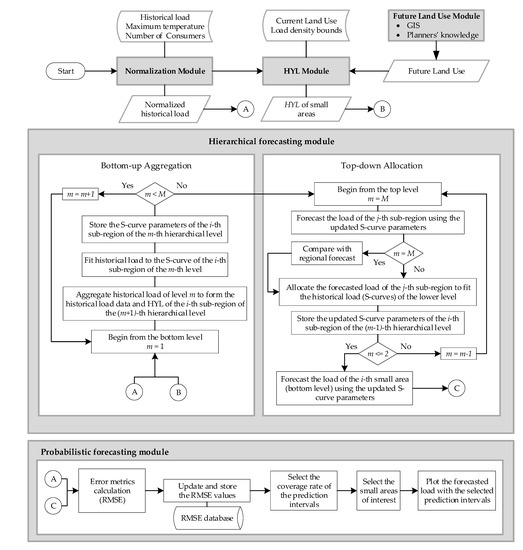
Figure 2.
Flowchart of the proposed probabilistic SLF method.
3.1. Normalization Module
The peak load depends on various conditions, such as the climate conditions (e.g., air temperature), the economy status, the number and the type of consumers in the service territory. The main factors that are affecting the electric demand of Athens, Greece, are investigated in [27]. Employing the approach of cooling and heating degree-days, the temperature seems to play the most important role in the electric load demand. In theory, the peak load is characterized by a linear trend, usually increasing, but the peak load curve is actually a zig-zag curve. Therefore, peak load data are normalized to smooth the deviations due to several random factors.
In this work, the available data are normalized with the method of least squares, which is mainly used in regression models and calculates the coefficients of a linear function that best fits on the historical data. For the sake of simplicity, in this work, two independent variables are considered (the maximum temperature that was recorded during the year t, , and the number of consumers in the service territory, Ct), as presented by Equation (2a). More independent variables that affect the peak load can also be incorporated in the multivariate regression model, e.g., the cooling and/or heating degree-days, the economic development of the service territory, and the mean value of the electric demand, according to the situation.
After the normalized peak load of the service territory in year t, , has been calculated, the normalized peak load of small area i in year t, , is calculated with Equation (2b).
3.2. Future Land Use Module
This module is mainly based on planners’ knowledge. The data of current land use, as well as the information for future development of the area under examination, are evaluated and the planners build the map of future land use. Sometimes, in order to predict the future land use, evolutionary algorithms or methods based on artificial intelligence are also adopted [10,11,12,13,14,15]. Although computer-based algorithms are useful and handy for future land use determination, data gathering and recollection of information such as land use classification, socioeconomic distribution, geospatial constraints (e.g., prohibited areas due to environmental restrictions) and information about points of interest of the service territory (e.g., municipal buildings, schools, hospitals, shopping malls, highways) are complemented by human knowledge. The land use is characterized accordingly considering the distance from those points of interest, decision maker’s experience and common sense. In case of evolutionary algorithms, the developed rules of evolution are also constructed by experts, but the future land use is a result of simulation based on these rules. Consequently, this module is human-based and experts’ presence is always mandatory for future land use determination.
3.3. Horizon Year Load Module
This module is based on the approach proposed in [18]. The HYL of the S-curves is calculated based on the data of current land use and that of future land use. Firstly, the load density of the service territory of each land use type is calculated according to the mathematical problem formulated by Equation (3a–c). The following Equation (3a–e) are applied for m = 1, which stands for the bottom level, and for , i.e., the last year of the historical data.
subject to:
The objective function, as shown in (3a), minimizes the deviation of the calculated load of small area i for the base year, , from the normalized historical load of the most recent year. Equation (3b) calculates the load of small area i for the base year based on the current land use and the unknown variable of load density, . The multiplication expresses the part of peak load of small area i for the base year that depends on land use of type k. The load density of the service territory is limited between a lower and an upper bound, as given in Equation (3c). The lower bound of Equation (3c) is always greater than zero, while both bounds denote the planner’s
Knowledge about the load density of the service territory for the base year as regards the land use of type k. For instance, the load density of vacant areas is set equal to zero and that of land use dedicated to transportation can be set between 0.2 and 5 MW/km2. This subproblem is a problem of quadratic programming (QP) and is solved using the CPLEX commercial solver of GAMS [28].
Consequently, given the load density of each type of land use for the base year, the HYL is calculated with Equation (3d–f), as follows.
Equation (3d) gives the difference between the normalized load and the calculated load of small area i for the most recent year (base year). The load density of the service territory of type k land use for the last year of the forecasting horizon can be estimated as a function of the load density for the base year, according to Equation (3e). The function is considered linear or polynomial and depends on the planners’ knowledge for future adoption of modern residential DERs or scheduled programs of energy efficiency. For instance, the load density of low-residential areas might increase due to the integration of domestic EV chargers and EHPs; the load density of commercial areas might decrease due to the adoption of energy efficiency programs and the load density of public utilities might increase due to the investment in public EV chargers. Equation (3f) is used for the final calculation of the HYL, which is greater than zero; the multiplication expresses the part of peak load of small area i in the year of saturation of the S-curve that depends on land use of type k. In this work, it is assumed that there is no change in the consumers’ behaviour and thus is equal to .
3.4. Hierarchical Forecasting Module
The forecasting module follows the hierarchical trending method proposed by T. Hong in the works [18,29]. This module is accordingly modified to improve the accuracy of the SLF. This hierarchical trending method includes two hierarchical processes: bottom-up aggregation and top-down allocation, as shown in Figure 3. In the former, an aggregation of data is occurred from lower levels to the upper levels, whereas, in the latter, the forecast of the upper levels is allocated to the lower levels. The number of levels is determined by the spatial resolution of the bottom level (level #1) and the number of areas that are aggregated to form the region of the upper level. For instance, in case the spatial resolution is selected such that it derives 256 small areas at level #1 (bottom level), and considering that four areas are grouped to form the region of the upper level, the number of levels is equal to 5, where the level #1 has 256 small areas, the level #2 has 64 sub-regions, the level #3 has 16 sub-regions, the level #4 has 4 sub-regions, and the level #5 is the service territory.
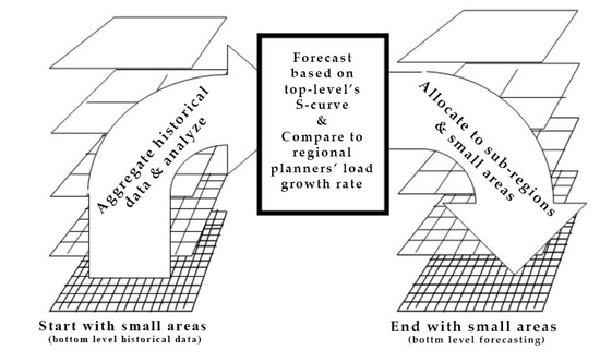
Figure 3.
Forecasting module: Bottom-up aggregation and top-down allocation [29].
3.4.1. Bottom-Up Aggregation
In this process, the aggregation of historical load and HYL is realized from the bottom level (level #1) to the upper levels (level #2 and higher). The main aim of this step is to fit the historical load to the S-curve of each small area (level #1) or sub-region (level #2 or higher). For reasons of clarity, hereafter, the term “small areas” is solely used for the bottom level (level #1) of the hierarchical procedure and the term “sub-regions” refers to the upper levels (level #2 or higher). For the bottom level, the data of historical load and those of HYL per small area are available from the available spatiotemporal database and the HYL module, respectively. As far as the higher levels are concerned, the aggregation to form the historical load and HYL data of the j-th sub-region of the (m + 1)-th hierarchical level is realized by applying Equation (4a) and Equation (4b), respectively.
For the calculation of the S-curve parameters of the i-th sub-region of the m-th level, the non-linear programming (NLP) problem that is formulated by Equation (5a–c) is solved. The state-of-the-art CONOPT4 commercial solver of GAMS [26] is employed for the solution.
subject to:
The objective function, Equation (5a), seeks to minimize the distance of the normalized historical load data of the i-th sub-region from the S-curve to optimally calculate the S-curve parameters. The slope parameter is always negative as limited by Equation (5b), while the ramp-up time parameter is limited according to Equation (5c). After the fitting of S-curve has been realized, the results (i.e., parameters of S-curve of each small area or sub-region i of each level m) are stored to be used as initialization of the top-down allocation process. Given the parameters of the S-curve of each small area or sub-region, the first forecast across the forecasting horizon can be realized.
3.4.2. Top-Down Allocation
With this process, the regional planners’ forecast is distributed on the sub-regions of the lower levels. In that setting, the corporation load forecasting, i.e., the estimated load growth rate of the wider area, is also taken into account and is compared with the forecasting based on the S-curve tuning of the bottom-up process, as described by Equation (6). Equation (6) is applied only for m = M, i.e., for the top level.
The S-curve parameters of the sub-regions or small areas of the lower level are re-calculated, so that the S-curve best fits both historical data and forecast results of the upper levels. To calculate the parameters of the S-curve of the small areas or sub-regions of the m-th level that belong to the j-th sub-region of the upper level (m+1), a non-linear programming problem is solved, as formulated by the Equation (7a–f). The following NLP mathematical model is solved for each sub-region j for each one of the upper levels starting from the top level (m = M) and ending on the level #2. The NLP problem of Equation (7a–f) is solved by the state-of-the-art CONOPT4 commercial solver of GAMS [26].
subject to:
The objective function, Equation (7a), seeks to minimize the weighted sum of the terms and , which in turn are weighted according to what planners want to achieve. For instance, in case the planner aims to fit the forecasted load to the historical load, the weighting factor is set much larger than ; in contrast, in case the planner aims to minimize the mismatch of the forecasted load to the forecasted load of the upper level, the weighting factor is set much larger than . In the case study presented in Section 5, the weighting factors and are set 0.95 and 0.05, respectively, to give more weight to minimize the error from the historical load of the same level rather than the forecasted load of the upper level. Equation (7b) gives the mismatch of the historical load from the S-curve, whereas Equation (7c) gives the mismatch of the forecasted load of the upper level from the S-curve. The forecasted load of the upper level is calculated by Equation (7d). The slope parameter is always negative and no less than a lower bound as given by Equation (7e), while the ramp-up time parameter is limited according to Equation (7f). The bounds of the parameters of S-curve are set by the planner’s wishes.
After the S-curve parameters of each small area of the bottom level have been calculated, the small areas’ load is calculated for the forecasting horizon. Optionally, the planners may select to further allocate the forecasted load to the distribution substations that are located in each small area. The allocation can be realized by a simplified approach, based on which the forecasted load of each small area is proportionally distributed to the corresponding distribution substations, i.e., to the distribution substations that each small area encompasses, according to Equation (8a). Alternatively, the forecasted load could be inversely distributed to the distribution substations in accordance to the utilization factor of the distribution substation, given in Equation (8b), taking into account the rule: “the higher the utilization factor is, the lower is the proportion of load to be distributed”.
3.5. Probabilistic Forecasting Module
In planning of distribution networks, probabilistic forecasting provides a better view than deterministic forecasting does. The planners can refer to probabilistic forecasting to make decisions based on less or more conservative scenarios. On the one hand, the deterministic forecasting produces point forecasts, without considering the upcoming deviations from the forecasted values, due to the forecasting errors that are always in presence. On the other hand, the planners shall use probabilistic forecasting methods, in which the forecasting error and its probability density function are considered. In this paper, the prediction intervals approach is adopted to define the probabilistic spatial load forecasting. In that setting, the spatial error of the deterministic hierarchical forecasting procedure (that of Section 3.4) is directly linked in a simple way with the upcoming new forecasted values.
According to [30], a prediction interval with a coverage rate α% is defined as a range of potential values for the future observations yt+h, computed based on past observations, such that the future observations yt+h will fall in this interval with probability α, where α [0, 1]. For example, for a prediction interval with a coverage rate of 90%, there is 90% probability for the future observations to belong in this prediction interval. Prediction intervals are usually based on the RMSE of the deterministic forecasting models, which provides an estimate of the standard deviation of the forecast error, as stated in [31]. In what follows, it is assumed that the forecast error of the h–th next year is normally distributed with zero mean and standard deviation , i.e., ~ N(0, ). Therefore, the upper bound and the lower bound of the prediction interval of the h–th next year can be constructed by applying the Equation (9a) and Equation (9b), respectively.
In Equation (9a,b), denotes the point-forecasts issued in year t for the h–th next year and z is the critical value of the standard normal distribution that gives the coverage rate of the prediction interval. For example, z = 3 gives a prediction interval with a coverage rate of 99.7% and z = 1 gives a prediction interval with a coverage rate of 86.6% [31]. The choice of z value depends on how conservative the planners are. It should be noted that the standard deviation of the forecast error depends on the lead time of the prediction.
The probabilistic forecasting module constructs the prediction intervals of the forecasting procedure based on the spatial error that is always in presence. The RMSE of the h–th next year is calculated and updated every year a new SLF is carried out. The formula that is used to calculate the RMSE is presented in Section 4. After the RMSE has been determined, the planner selects the values of z to form the prediction intervals of the extrapolation.
4. Spatial Load Forecasting Assessment Metrics
4.1. Assessment Metrics of Point-Forecasts
The RMSE, as well as the mean absolute error (MAE), can be used in deterministic SLF to measure the spatial error along the small areas of the service territory, as mentioned in [7]. The spatial error metrics RMSE and MAE are defined as given in Equation (10a) and Equation (11a), respectively, where , and N is the number of sub-regions (or small areas) used for the calculations. Their normalized values are calculated by dividing the values of RMSE and MAE with the average actual load of the service territory, as indicated by Equation (10b) and Equation (11b), respectively.
4.2. Assessment Metrics of Probabilistic Forecasts
The error metric that is used for the assessment of the probabilistic part of SLF that takes place is the prediction interval coverage probability (PICP) [32]. PICP is calculated by Equation (12a,b), where is the number of small areas.
PICP is related to the validity of the prediction intervals and is directly compared with the prediction interval nominal coverage (PINC). It is worth noting that PINC is the set coverage rate of the prediction interval, whereas PICP reflects the posterior coverage probability of the prediction interval. Theoretically, PICP should be very close to or greater than PINC. Otherwise, if this criterion is not satisfied, the constructed prediction intervals are not reliable and their credibility is questionable [33].
Another metric that is introduced to measure the error of the constructed prediction intervals is the probabilistic RMSE (p-RMSE) [34]. This metric aims to quantify the error in cases the target values, i.e., the measured actual load, exceed the bounds of the prediction interval that is selected by the planner. For instance, if the planner relies on a prediction interval with a coverage rate of 80%, all target values that lie in this interval are approved and the remaining are used for the calculation of p-RMSE, which is accompanied by a probability of 20%. The value of p-RMSE is calculated by Equation (13a), where is the probabilistic error as defined by Equation (13b).
5. Case Study, Results, and Discussion
5.1. The Service Territory under Examination
The proposed methodology is applied on a real-world distribution network, located at the region of Attica, Greece. The distribution network consists of 355 distribution substations that are spanned across a coastal area of about 64 km2, approximately 24 km2 of which are covered by sea. The spatial resolution is set to 0.25 km2 (squares of 0.5 km side) and consequently the service territory is divided into 256 small square areas (level #1). The total installed capacity of the distribution substations is 188 MVA. The peak load in the base year (year 1999) is approximately 92.2 ΜW. The regional planners estimate an annual load growth rate of 1.6% and the 20-year horizon load of the service territory is expected to exceed the value of 125 MW.
The land use is classified by nine different land use types as given in Table 1. The current land use and the future land use are those presented in the second and the third column of Table 1, respectively. The minimum and maximum values of load density per land use type, which are determined according to planner’s knowledge, are given in the fourth and the fifth column of Table 1, respectively. The data for the current land use (Figure A1) and the future land use (Figure A2) for the land use types under consideration are provided in detail in Appendix A.

Table 1.
Land use types of the service territory.
Figure 4a shows the allocation of the actual load density in year 1999 (base year) given in MW/km2. The values of load of each small area could be also expressed in MW; the choice depends on how the reader wishes to interpret the results, e.g., giving the results in MW/km2 makes the comparison between different hierarchical levels easier. The cells with grey color represent the area covered by sea and the rest cells are colored depending on the values of load density according to the color scale (MW/km2) on the right of Figure 4a. The aerial view of the service territory, as captured by satellite, is shown in Figure 4b. The spatial variability of loads in the base year can be explained by referring to Figure A1. The service territory is divided into four main zones, which actually are the sub-regions of level #4, as indicated by the circles in Figure 4a. The city centre of the service territory, which is characterized by intense commercial, retail and business activity, is located at the northwestern area (Zone A), where high values of load density are observed. The rest areas are mainly characterized by residential land use (Zone C and Zone D). There is also a second area of interest that is located at the short peninsula at southwest (Zone B), where a luxury grand resort and other hotel facilities are located.
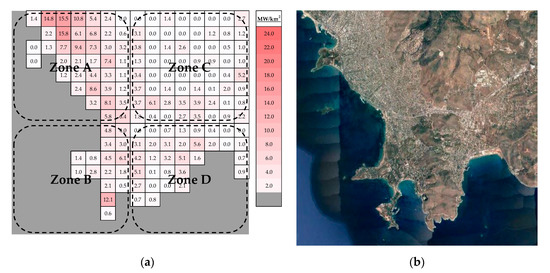
Figure 4.
(a) Actual load density in year 1999 (base year); (b) Aerial view of the service territory.
A database with the peak load of 30 years, from 1990 to 2019, is used for the demonstration of the proposed methodology. The first 10 years are used as input data (historical data), whereas the remaining 20 years, from 2000 to 2019 (forecasting horizon) serve as the actual data to measure the spatial error. For the top-down allocation procedure of the hierarchical forecasting, the weighting factors and are set 0.95 and 0.05, respectively. A brief sensitivity analysis was carried out and these are the values that prove better performance. For sure, the selection of the weighting factors depends on the case study and should always be chosen carefully. The time elapsed for the execution of the case study with the proposed SLF methodology is about 2 min. It is worth noting that the execution time is expected much larger in cases with thousands of small areas at the bottom level. The computational effort depends on the selected spatial resolution, the size of the service territory, and the bounds of the S-curve parameters on the NLP optimization parts.
5.2. Simulation Methods
Along with the proposed P-SLF method, a BaU method is adopted for comparison purposes. The BaU methods is compared with the P-SLF method to quantify its performance. The simulation methods are described as follows:
- P-SLF method: The proposed method. In this method, firstly, the hierarchical forecasting module, described in Section 3.4, produces the point forecasts across the forecasting horizon, and subsequently the prediction intervals are constructed based on the RMSE values that have been calculated from the comparison between the available actual and forecasted values, without loss of generality. In fact, the RMSE values are calculated based on the past predictions and the historical data.
- BaU method: In this method, the regional planners’ load growth rate of the service territory is proportionally allocated to all the small areas of the bottom level. Subsequently, in this method, the prediction intervals are constructed based on higher RMSE values, as was a priori expected.
5.3. Results and Discussion
5.3.1. Load Density of the Service Territory
Based on the mathematical formulation of Section 3.3, the load density of service territory per land use type is calculated for the base year, as presented in Table 2. The load density of the base year is considered equal to the load density of the last year of the forecasting horizon , as there are no announcements for energy efficiency programs or forecasting for adoption of EVs and EHPs in the area under examination until the end of 2020.
Table 2.
Load density of the service territory per land use type (base year).
5.3.2. Assessment of Point-Forecasts
The deterministic part is evaluated by comparing the results presented in Figure 5a–d. The same color scale with that of Figure 4a is used to visualize the results. Figure 5a depicts the actual load density per small area in year 2019. The spatial variability of loads can be explained by referring to Figure A2, which depicts the anticipated future land use in year 2019. The values of Figure 5a are used as reference for the calculation of the RMSE of the last year of the forecasting horizon (year 2019). Figure 5b depicts the forecasted load density in year 2019 by applying the proposed P-SLF method, whereas Figure 5c depicts the forecasted load density in year 2019 by applying the BaU method. In Figure 5d, the normalized values of absolute error of the forecasted load for each small area in year 2019 are presented. The values of Figure 5d, given in percentage, are expressed in relation to the average actual load density of the service territory, according to Equation (14).
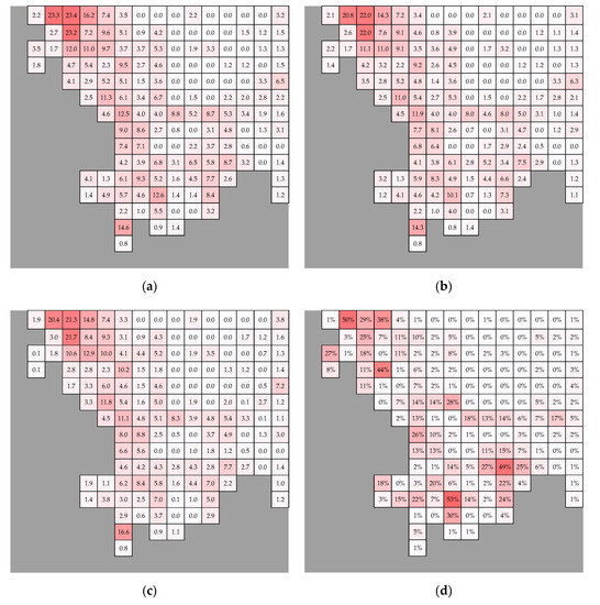
Figure 5.
(a) Actual load density in year 2019; (b) Forecasted load density in year 2019 (P-SLF method); (c) Forecasted load density in year 2019 (BaU method); (d) Normalized absolute error in year 2019 (P-SLF method).
From Figure 5d, it is concluded that the prediction error is not equally distributed over the service territory. There are several small areas with significantly low prediction error varying from 1% to 10%, but outliers are also present, e.g., the red-highlighted values over 50%. The forecast error, which is spatially visualized in the map, can be summarized by the values of RMSE and MAE. The values of RMSE and MAE are calculated for every year of the forecasting horizon. Table 3 shows the values of RMSE and MAE for the last year of the forecasting horizon (year 2019).
Table 3.
RMSE and MAE calculated for year 2019.
From Table 3, it is concluded that the proposed P-SLF has much better performance than the BaU method. When it comes to prediction of future feeder loads, BaU method shows a MAE of 19.1%, while P-SLF has a MAE of 8.8%. RMSE of BaU method is 28.1%, in comparison with P-SLF method that performs a RMSE value of 14.2%. This goes to show that there are more outliers in BaU method than in the P-SLF method. This is something that highlights the importance of SLF, particularly when there is high interest for planning of distribution networks.
With a deeper examination of the results, the findings are getting more interesting. Since RMSE is only slightly greater than MAE in Zone C, the method makes relatively few big mistakes than its average in this zone. Comparing RMSE and MAE of Zone D, it can be concluded that Zone D is by far the area with higher values of errors. The RMSE is an error metric that inherently gives a relatively high weight to large errors. The RMSE values will always be larger or equal to those of MAE. The greater difference between them, the greater the variance in the individual errors in the sample.
5.3.3. Assessment of Probabilistic Forecasts
Figure 6a–d show the evolution of the load (given in MW) across the forecasting horizon in four representative small areas of the service territory. Each of the selected small areas (that of Figure 6a–d) is interesting for different reasons. For example, Figure 6a (referring to the small area of the 2nd row and the 4th column of the grid) shows that the proposed method initially overestimates the actual load (from 2000 to 2007), and subsequently underestimates it (from 2008 to 2019). In Figure 6b, the load is persistently underestimated and lies near the upper bounds of the prediction interval of 95%. The annual load time-series of Figure 6c exceeds the upper bounds of the prediction interval of 95%. One can state that this is due to the false estimation of the HYL in this small area. The load of small area of Figure 6d was forecasted with relatively high accuracy.
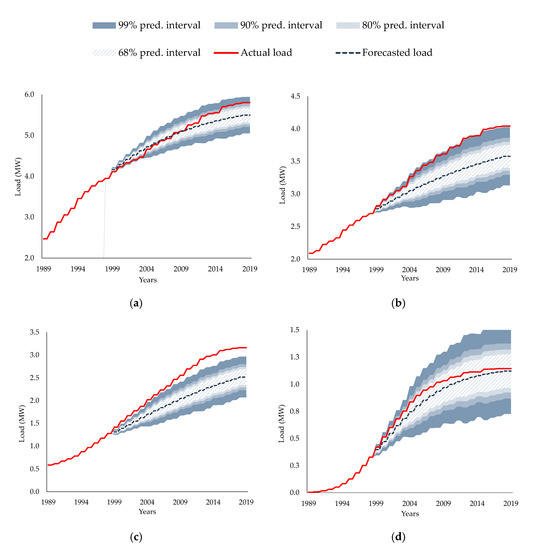
Figure 6.
Probabilistic load forecasting of representative small areas considering the RMSE of the total area (service territory): (a) small area {2, 4} (Small area {x, y} denotes the square located in the x-th row and the y-th column of the grid of the service territory); (b) small area {1, 5}; (c) small area {12, 9}; (d) small area {4, 9}.
Table 4 gives the results of PICP and p-RMSE to evaluate the probabilistic part of the proposed method. PICP values are greater than PINC for the prediction intervals of 50%, 68%, 75%, 80% and 90%, and thus these prediction intervals are approved. PICP values of the prediction intervals 95% and 99% are slightly lower than the corresponding PINC. Though the general rule that evaluates the validity of prediction intervals (PICP ≥ PINC), PICP is close to PINC and is not discarded.
Table 4.
PICP (across the forecasting horizon) and p-RMSE (for year 2019).
The values of p-RMSE help the reader understand better the PICP results and also aim to quantify the distance of those target values that are not covered by the constructed prediction intervals. More specifically, if the planner selects PINC of 75%, the actual load of a small area may lie outside of the bounds of the prediction interval by 7% with probability of 25%. It depends on how much crucial the prediction error is in a specific small area. For instance, the planner may wish to select wider prediction intervals in small areas that are unoccupied (or present low load density), because there is higher chance of development, and therefore there is higher need for installation of new substations or LV feeders. On the other hand, saturated small areas are usually equipped with more distribution substations, which in turn can accommodate higher loads than expected.
6. Conclusions
This paper proposes a novel probabilistic framework for SLF based on a hierarchical forecasting method that uses the well-known S-curves for fitting the historical load data. It is worth noting that this work takes advantage of the spatial error, which is calculated by means of the root-mean-squared error along the service territory, to construct the prediction intervals of the proposed P-SLF. The probabilistic forecasting part, in turn, is introduced to serve as a decision-making tool for regional planners and distribution network operators, who wish to choose between an ordinary and a more conservative forecasting. The proposed method is applied on a real-world distribution network and its effectiveness is validated by comparing the results of the proposed method with the results obtained by a BaU approach. Moreover, the error metrics of PICP and p-RMSE are adjusted to quantify the spatial error in the view of probabilistic SLF.
The findings prove that the deterministic part of the proposed method shows high spatial accuracy and reduces the spatial error compared to a BaU approach. As far as the probabilistic part is concerned, PICP and p-RMSE have valid values making the P-SLF a reliable probabilistic tool. It should be noted that any examination of the prediction errors should always be carefully carried out by the planners.
As regards proposals for future work, there is room for further investigation in the field of SLF, especially in areas/cities with high urban development. For example, the method can be enriched with the addition of an evolutionary algorithm that dynamically determines the future land use across the service territory for every year of the forecasting horizon. In that setting, the historical load data and the regional forecasting would better fit the S-curve of each small area. What is more, there is interest for further development of SLF models that consider the adoption of new technologies, such as EVs, EHPs, PVs and energy efficiency programs. The quantification of the benefits from more accurate SLF methods is also valuable, but not within the scope of this paper; however, it is strongly recommended as a future work.
Author Contributions
V.E. developed the methodology and the software, made the validation, and wrote the paper; P.K. contributed in the validation of the method and reviewed the paper. P.G. managed the project and reviewed the paper. All authors have read and agreed to the published version of the manuscript.
Funding
This research has been co-financed by the European Union and Greek national funds through the Operational Program Competitiveness, Entrepreneurship and Innovation, under the call RESEARCH–CREATE–INNOVATE (project code: T1EDK-00450).
Acknowledgments
The authors express their gratitude to the Hellenic Electricity Distribution Network Operator (HEDNO) for providing the network data.
Conflicts of Interest
The authors declare no conflict of interest.
Nomenclature
| A. Acronyms | |
| BaU | Business-as-usual |
| DER | Distributed energy resource |
| DNO | Distribution network operator |
| EHP | Electric heat pump |
| EV | Electric vehicle |
| GIS | Geographical information system |
| HV | High voltage |
| HYL | Horizon year load |
| LV | Low voltage |
| LTLF | Long-term load forecasting |
| MAE | Mean absolute error |
| MV | Medium voltage |
| NLP | Non-linear programming |
| PICP | Prediction interval coverage probability |
| PINC | Prediction interval nominal coverage |
| P-SLF | Probabilistic spatial load forecasting |
| p-RMSE | Probabilistic root-mean squared error |
| PV | Photovoltaic |
| QP | Quadratic programming |
| RMSE | Root-mean squared error |
| SLF | Spatial load forecasting |
| STLF | Short-term load forecasting |
| B. Sets and indices | |
| Types of land use, indexed by k | |
| M | Levels of the SLF hierarchical procedure, indexed by m |
| Years of the available historical data, indexed by t | |
| Years of the forecasting horizon, indexed by t | |
| Sub-regions of level m (small areas of level m = 1), indexed by i, running from 1 to | |
| Sub-regions of level m (small areas of level m = 1) belonging to the j-th sub-region of the upper level, indexed by i, running from 1 to | |
| C. Parameters | |
| Maximum temperature recorded during year t [°C] | |
| Number of electrified customers in the service territory in year t | |
| Current land use of small area i of land use type k [km2] | |
| Minimum value of load density of land use type k [MW/km2] | |
| Maximum value of load density of land use type k [MW/km2] | |
| Minimum value of ramp-up time parameter of the S-curve | |
| Maximum value of ramp-up time parameter of the S-curve | |
| Future land use of small area i of land use type k [km2] | |
| Historical peak load (raw data) of distribution substation tr in year t [MW] | |
| Historical peak load (raw data) of sub-region i of level m in year t [MW] | |
| Normalized historical peak load of sub-region i of level m in year t [MW] | |
| Actual peak load of sub-region i of level m in year t [MW] | |
| Utilization factor of distribution substation tr in year t [%] | |
| Weighting factors of top-down allocation procedure | |
| D. Variables | |
| Coefficients of the linear function of load normalization | |
| Error of point-forecast of small area i [MW] | |
| Error of probabilistic forecast based on prediction intervals of small area i [MW] | |
| Slope parameter of the S-curve of sub-region i of level m | |
| Ramp-up time parameter of the S-curve of sub-region i of level m | |
| Load density of land use type k [MW/km2] | |
| Difference between the normalized historical load and the calculated load of small area i for the base year [MW] | |
| Horizon year load of sub-region i of level m [MW] | |
| Calculated load of small area i for the base year [MW] | |
| Forecasted peak load of distribution substation tr in year t [MW] | |
| Forecasted peak load of sub-region i of level m in year t [MW] | |
Appendix A
Figure A1 presents the current land use for the base year (year 1999), for each type of land use.

Figure A1.
Current land use as percentage (%) of the small area’s size (a) sum of business and commercial land use; (b) industrial land use; (c) low residential land use; (d) high residential land use; (e) sum of governmental and utilities land use; (f) transportation land use.
Figure A1.
Current land use as percentage (%) of the small area’s size (a) sum of business and commercial land use; (b) industrial land use; (c) low residential land use; (d) high residential land use; (e) sum of governmental and utilities land use; (f) transportation land use.

Figure A2 presents the future land use for the last year of the forecasting horizon (year 2019), for each type of land use.

Figure A2.
Future land use as percentage (%) of the small area’s size (a) sum of business and commercial land use; (b) industrial land use; (c) low residential land use; (d) high residential land use; (e) sum of governmental and utilities land use; (f) transportation land use.
Figure A2.
Future land use as percentage (%) of the small area’s size (a) sum of business and commercial land use; (b) industrial land use; (c) low residential land use; (d) high residential land use; (e) sum of governmental and utilities land use; (f) transportation land use.

References
- Willis, H.L.; Northcote-Green, J.E.D. Spatial electrical load forecasting: A tutorial review. Proc. IEEE 1983, 71, 232–253. [Google Scholar] [CrossRef]
- Hong, T.; Fan, S. Probabilistic electric load forecasting: A tutorial review. Int. J. Forecast. 2016, 32, 914–938. [Google Scholar] [CrossRef]
- Evangelopoulos, V.A.; Georgilakis, P.S. Optimal distributed generation placement under uncertainties based on point estimate method embedded genetic algorithm. IET Gener. Transmiss. Distrib. 2014, 8, 389–400. [Google Scholar] [CrossRef]
- Koutsoukis, N.C.; Georgilakis, P.S. A chance-constrained multistage planning method for active distribution networks. Energies 2019, 12, 4154. [Google Scholar] [CrossRef]
- Li, R.; Wang, W.; Chen, Z.; Jiang, J.; Zhang, W. A review of optimal planning active distribution system: Models, methods, and future researches. Energies 2017, 10, 1715. [Google Scholar] [CrossRef]
- Koutsoukis, N.C.; Georgilakis, P.S.; Hatziargyriou, N.D. Multistage coordinated planning of active distribution networks. IEEE Trans. Power Syst. 2017, 33, 32–44. [Google Scholar] [CrossRef]
- Willis, H.L. Spatial Electric Load Forecasting, 2nd ed.; Marcel Dekker: New York, NY, USA, 2002. [Google Scholar]
- Heymann, F.; Melo, J.D.; Martínez, P.D.; Soares, F.; Miranda, V. On the emerging role of spatial load forecasting in transmission/distribution grid planning. In Proceedings of the Mediterranean Conference on Generation, Transmission, Distribution and Energy Conversion (MEDPOWER 2018), Dubrovnik, Croatia, 12–15 November 2018. [Google Scholar]
- Sasmono, S.; Sinisuka, N.I.; Atmopawiro, M.W.; Darwanto, D. Macro demand spatial approach (MDSA) at spatial demand forecasting for transmission system planning. Int. J. Electr. Eng. Inform. 2015, 7, 193–206. [Google Scholar] [CrossRef]
- Carreno, E.M.; Padilha-Feltrin, A. Evolutionary heuristic to determine future land use. In Proceedings of the IEEE Power Energy Society General Meeting (PES GM), Pittsburgh, PA, USA, 20–24 July 2008. [Google Scholar]
- Carreno, E.M.; Rocha, R.M.; Padilha-Feltrin, A. A Cellular automaton approach to spatial electric load forecasting. IEEE Trans. Power Syst. 2011, 24, 532–540. [Google Scholar]
- He, Y.; Yang, W.; Zhan, Y.; Li, D.; Li, F. Urban electric load forecasting using combined cellular automata. J. Comput. 2009, 4, 1209–1215. [Google Scholar] [CrossRef]
- He, Y.X.; Zhang, J.X.; Xu, Y.; Gao, Y.; Xia, T.; He, H.Y. Forecasting the urban power load in China based on the risk analysis of land-use change and load density. Int. J. Electr. Power Energy Syst. 2015, 73, 71–79. [Google Scholar] [CrossRef]
- Melo, J.D.; Padilha-Feltrin, A.; Carreno, E.M. Multi-agent simulation of urban social dynamics for spatial load forecasting. IEEE Trans. Power Syst. 2012, 27, 1870–1878. [Google Scholar] [CrossRef]
- Melo, J.D.; Carreno, E.M.; Padilha-Feltrin, A. Multi-Agent framework for spatial load forecasting. In Proceedings of the IEEE Power Energy Society General Meeting (PES GM), Detroit, MI, USA, 24–28 July 2011. [Google Scholar]
- Vasquez-Arnez, R.L.; Jardini, J.A.; Casolari, R.; Magrini, L.C.; Semolini, R.; Pascon, J.R. A methodology for electrical energy forecast and its spatial allocation over developing boroughs. In Proceedings of the IEEE Transmission and Distribution Conference and Exposition, Chicago, IL, USA, 21–24 April 2008. [Google Scholar]
- Morales, D.X.; Besanger, Y.; Moscoso, S.A.; Pesantez, P.A. Development of a spatial load-forecasting module for optimizing planning of electricity supply. In Proceedings of the IEEE Innovative Smart Grid Technologies Latin America (ISGT Latin America), Quito, Ecuador, 20–22 September 2017. [Google Scholar]
- Hong, T.; Hsiang, S.M.; Xu, L. Human-machine co-construct intelligence on horizon year load in long term spatial load forecasting. In Proceedings of the IEEE Power Energy Society General Meeting (PES GM), Calgary, AB, Canada, 26–30 July 2009. [Google Scholar]
- Melo, J.D.; Carreno, E.M.; Calvino, A.; Padilha-Feltrina, A. Determining spatial resolution in spatial load forecasting using a grid-based model. Electr. Power Syst. Res. 2014, 111, 177–184. [Google Scholar] [CrossRef]
- Melo, J.D.; Carreno, E.M.; Padilha-Feltrin, A. Estimation of a preference map of new consumers for spatial load forecasting simulation methods using a spatial analysis of points. Int. J. Electr. Power Energy Syst. 2015, 67, 299–305. [Google Scholar] [CrossRef]
- Melo, J.D.; Carreno, E.M.; Padilha-Feltrin, A.; Minussi, C.R. Grid-based simulation method for spatial electric load forecasting using power-law distribution with fractal exponent. Int. Trans. Electr. Energ. Syst. 2016, 26, 1339–1367. [Google Scholar] [CrossRef]
- Hong, T.; Pinson, P.; Fan, S. Global energy forecasting competition 2012. Int. J. Forecast. 2014, 30, 357–363. [Google Scholar] [CrossRef]
- Avramidis, I.I.; Evangelopoulos, V.A.; Georgilakis, P.S.; Hatziargyriou, N.D. Demand side flexibility schemes for facilitating the high penetration of residential distributed energy resources. IET Gener. Transmiss. Distrib. 2018, 12, 4079–4088. [Google Scholar] [CrossRef]
- Bernards, R.; Morren, J.; Slootweg, H. Development and implementation of statistical models for estimating diversified adoption of energy transition technologies. IEEE Trans. Sustain. Energy 2018, 9, 1540–1554. [Google Scholar] [CrossRef]
- Heymann, F.; Silva, J.; Miranda, V.; Melo, J.; Soares, F.J.; Padilha-Feltrin, A. Distribution network planning considering technology diffusion dynamics and spatial net-load behavior. Int. J. Electr. Power Energy Syst. 2019, 106, 254–265. [Google Scholar] [CrossRef]
- Hong, T.; Wilson, J.; Xie, J. Long term probabilistic load forecasting and normalization with hourly information. IEEE Trans. Smart Grid 2014, 5, 456–462. [Google Scholar] [CrossRef]
- Psiloglou, B.E.; Giannakopoulos, C.; Majithia, S.; Petrakis, M. Factors affecting electricity demand in Athens, Greece and London, UK: A comparative assessment. Energy 2009, 34, 1855–1863. [Google Scholar] [CrossRef]
- General Algebraic Modeling System (GAMS), Release 25.1.3; High-Level Modeling System for Mathematical Optimization; GAMS Develop. Corp.: Fairfax, VA, USA, 2018.
- Hong, T. Spatial Load Forecasting Using Human Machine Co-construct Intelligence Framework. Master’s Thesis, North Carolina State University, Raleigh, NC, USA, 2008. [Google Scholar]
- Morales, J.M.; Conejo, A.J.; Madsen, H.; Pinson, P.; Zugno, M. Integrating Renewables in Electricity Markets-Operational Problems; Springer: New York, NY, USA, 2014; pp. 21–26. [Google Scholar]
- Makridakis, S.G.; Wheelwright, S.C.; Hyndman, R.J. Forecasting: Methods and Applications, 3rd ed.; Wiley: New York, NY, USA, 1997; pp. 52–54. [Google Scholar]
- Khosravi, A.; Nahavandi, S.; Creighton, D. Construction of optimal prediction intervals for load forecasting problems. IEEE Trans. Power Syst. 2010, 25, 1496–1503. [Google Scholar] [CrossRef]
- Quan, H.; Srinivasan, D.; Khosravi, A. Uncertainty handling using neural network-based prediction intervals for electrical load forecasting. Energy 2014, 74, 916–925. [Google Scholar] [CrossRef]
- Zuniga-Garcia, M.A.; Santamaría-Bonfil, G.; Arroyo-Figueroa, G.; Batres, R. Prediction interval adjustment for load-forecasting using machine learning. Appl. Sci. 2019, 9, 5269. [Google Scholar] [CrossRef]


© 2020 by the authors. Licensee MDPI, Basel, Switzerland. This article is an open access article distributed under the terms and conditions of the Creative Commons Attribution (CC BY) license (http://creativecommons.org/licenses/by/4.0/).