An Overview of Modelling Techniques and Control Strategies for Modular Multilevel Matrix Converters

Abstract

The Modular Multilevel Matrix Converter is a relatively new power converter topology appropriate for high-power Alternating Current (AC) to AC purposes. Several publications in the literature have highlighted the converter capabilities such as modularity, control flexibility, the possibility to include redundancy, and power quality. Nevertheless, the topology and control of this converter are relatively complex to design and implement, considering that the converter has a large number of cells and floating capacitors. Therefore multilayer nested control systems are required to maintain the capacitor voltage of each cell regulated within an acceptable range. There are no other review papers where the modelling, control systems and applications of the Modular Multilevel Matrix Converter are discussed. Hence, this paper aims to facilitate further research by presenting the technology related to the Modular Multilevel Matrix Converter, focusing on a comprehensive revision of the modelling and control strategies.

1. Introduction

Modular Multilevel Cascaded Converters (MMCCs) have developed as one of the most attractive alternatives for high-power applications since its introduction at the beginning of the 2000s [1]. Initially, MMCCs were proposed for High Voltage Direct Current (HVDC) transmission applications, but lately, they have been introduced into other applications such as Static Synchronous Compensators (STATCOM) [2,3,4], Wind Energy Conversion Systems (WECS) [5,6], and drives [7,8].

Some of the advantages that have strengthened the use of MMCCs are their expandable and flexible structure, high efficiency, robustness, fault tolerance, and high power quality [9]. For instance, if a larger nominal voltage is required, more power-cells can be cascaded in each cluster. Moreover, if robustness is necessary, redundancy can be easily provided by including a number of additional cells in each cluster, which can be used to replace those damaged or in a faulty condition.

MMCCs are topologies characterised by the cascade connection of Half-Bridge or Full-Bridge power cells [10,11]. However, the implementation of MMCCs is not limited to use only these power cells, and other power cell topologies can be considered as proposed in [12]. The connection of clusters and power-cells lead to different MMCCs topologies, for instance the Modular Multilevel Converter (MMC or $M^{2}C$) also known as Marquardt Converter [1,13], the Hexverter [14,15], the PI Converter [16], the Hybrid Converter [17,18,19], the Modular Multilevel Converter ($M^{3}C$, see Figure 1), and other power electronic topologies discussed in [10,20]. In [11], a useful overview and classification of the converters in the MMCC family is presented.

The $M^{2}C$ is the most well-established topology among MMCCs. The $M^{2}C$ is an AC-DC converter composed of six clusters formed by the n cascaded power-cell. Despite the $M^{2}C$ development, other MMCCs topologies have gained popularity. For instance, the Hexverter and the $M^{3}C$ have been studied and proposed for AC-AC applications [13,14]. In particular, the $M^{3}C$ has been advantageously compared with other power electronic topologies and it is recommended for low-speed high-power applications [11,21,22].

Unlike the converter proposed by the Robicon Corporation (now part of Siemens), where the capacitor voltages of the power-cells are imposed by voltage sources (see [23]), the capacitor voltage of each power-cell is floating in the $M^{3}C$. Then, the power-cells could charge–discharge during the operation of the converter, and the regulation of the floating capacitor voltages becomes one of the essential control purposes. This could be especially complicated when feeding a motor drive in variable-speed applications [24,25].

The control complexity, plus the high component count required for industrial implementations, have hindered the commercial and research development of the $M^{3}C$. According to [8], just four research groups have reported experimental results obtained using an $M^{3}C$ prototype. Nevertheless, it is expected that shortly the $M^{3}C$ could compete with high-power cyclo-converter-based drives [10], and be used for high-power wind turbines [26,27]. Consequently, research on the $M^{3}C$ is a promising area that requires further research.

The $M^{3}C$ has nine clusters of series-connected full-bridge power-cells enabling the direct connection of two AC ports, as shown in Figure 1. The floating capacitor voltage in the $M^{3}C$ must be regulated using circulating currents (or other methodologies) to ensure the stable operation of the converter in the whole operating range [11]. As aforementioned, this converter is appropriate for low-speed and high-power applications because lower circulating currents, in comparison to those required in the $M^{2}C$, are required to regulate the capacitor voltage oscillations [8,28]. However, the $M^{3}C$ has problems operating at a synchronous frequency (similar or equal input/output port frequencies) because considerable capacitor voltage oscillations can be produced at this operating point [11,29,30].

Owing to this problem, the operation of the $M^{3}C$ can be categorised into the following modes: the Different Frequencies Mode (DFM) and the Equal Frequencies Mode (EFM) [27]. The $M^{3}C$ is considered to operate in DFM when the input-port frequency is distinct from the output-port frequency (i.e., higher or lower than a given threshold). In DFM, the control of the floating capacitor of the converter is simpler to realise because the capacitor voltage oscillations are relatively low. Consequently, most of the current research development on the $M^{3}C$ has been proposed for DFM operation [13,24,27]. On the other hand, the $M^{3}C$ operates in EFM when the absolute value of the input-port frequency is approaching the output-port frequency. In EFM, more sophisticated control strategies are usually required to reduce large oscillations in the floating capacitor voltages [31,32].

This paper provides an extensive and thorough review of the state-of-the-art of the $M^{3}C$, focusing on a comprehensive revision of modelling and control strategies.

The contributions in this paper are:

• To the best of the author’s knowledge, this is the first review paper discussing and comparing modelling methodologies, and control of the $M^{3}C$. In the field of MMCCs, there are other review papers available. For instance, various papers deal with modelling and control of the $M^{2}C$ [2,9,20,33,34]. There are also some review papers related to the Hexverter power converter [14], and performance comparison between the $M^{2}C$ and $M^{3}C$ for drive applications [8,28]. However, none of those papers fully describe the operation and control of the $M^{3}C$ for DFM and EFM operation. Neither control nor modelling approaches have been thoroughly discussed before.
• The problem of the floating capacitor voltages in the $M^{3}C$ is detailed, and numerical analysis is presented to describe and map the nature of the voltage oscillations as a function of the electrical parameters at the input and output port of the converter.
• In this work, the modelling methodologies and control strategies reported in the literature (for the $M^{3}C$) are discussed and classified in terms of the type of linear transformation used to represent the currents and voltages of the converter.
• The currently proposed control strategies for EFM operation are revised and discussed, and the available methods for the selection of the common-mode voltage and circulating currents are fully described.
• Finally, future trends are presented to highlight the unsolved problems related to the $M^{3}C$ control and future research topics.

The rest of this paper is organised as follows. The $M^{3}C$ topology and an analysis of the floating capacitor voltage oscillations are included in Section 2. Then, an extensive revision of modelling proposals for the $M^{3}C$ is presented in Section 3. The modelling of the converter is studied using the Double$-\alpha \beta \gamma$ and $\Sigma \Delta$ Double$-\alpha \beta \gamma$ frames. Section 4 presents a summary of the control strategies proposed in the literature, discussing different approaches, modulation techniques and main challenges to achieve proper operation of the converter in DFM and EFM operation. Future trends and possible research areas related to the $M^{3}C$ control are outlined in Section 5. Finally, an appraisal of the control systems and topologies discussed in this paper are presented in the conclusions.

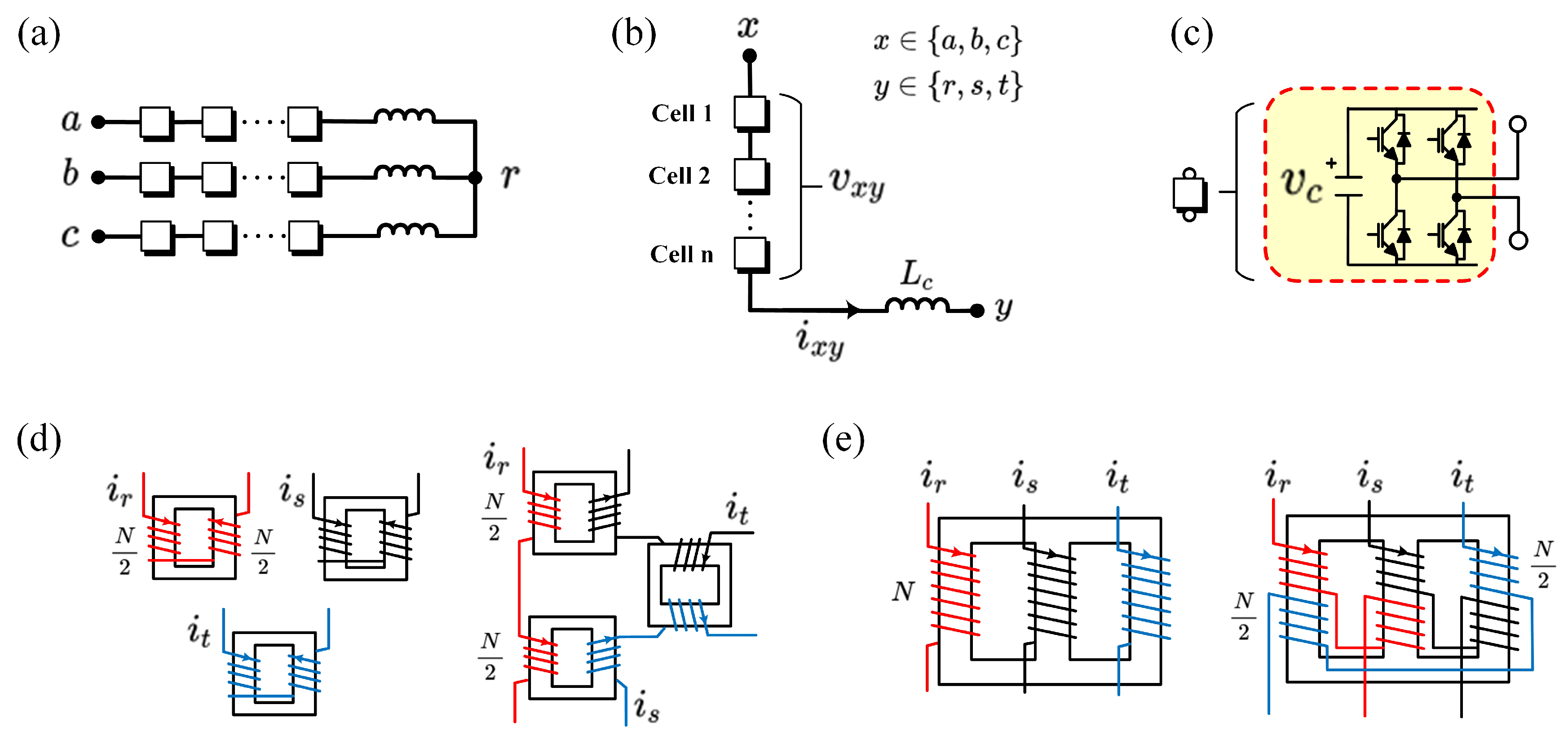
2. The Modular Multilevel Matrix Converter

The circuit of the $M^{3}C$ is shown in Figure 1. This converter has also been referred to as Direct MMC [35], or Modular Multilevel Cascade Converter based on Triple-Star Bridge Cells (MMCC-TSBC) [11]. The $M^{3}C$ is composed of three sub-converters, or single-phase $M^{3}C$, linking two AC three-phase systems. As shown in Figure 2a, each sub-converter comprises three clusters connecting the three phases of the input system (i.e., phases $a,b,c$), to one phase of the output system (e.g., phase r). The composition of a single cluster is presented in Figure 2b, which comprises n power-cells connected in series to an inductor $L_c$. The power-cell is formed by a Full-Bridge connected to a floating capacitor, as shown in Figure 2c, avoiding, therefore, the use of external DC voltage sources.

The $M^{3}C$ requires an inductor in each cluster to avoid short circuits between the clusters, and most importantly to provide controllability of the cluster currents and to reduce their ripple. These inductors can have different configurations, as shown in Figure 2d,e. The most simple setup is to use three independent inductors per each sub-converter (see Figure 2a) [36]. Coupled inductors have been proposed to reduce size and weight. For instance, the use of three-phase three-core coupled inductors or three-phase single-core coupled inductors have been introduced in [7,13,37]. These magnetically coupled configurations are characterised by having zero equivalent inductance from the output currents point of view, and only the input and circulating currents produce magnetic flux. Therefore, the output currents do not have to be considered for the sizing of the magnetic cores, and smaller and less expensive inductor designs can be employed to develop the $M^{3}C$. Nevertheless, further size and weight reductions can be achieved by using the three-phase single-core inductor configurations depicted in Figure 2e. As analysed in [37], these inductor configurations allow the total weight to be reduced to almost 32% of the one obtained with the nine independent inductors for the same cluster inductance.

Floating Capacitor Voltage Oscillations

As no external sources are used to impose the voltages in the power cells of the $M^{3}C$, the floating capacitor voltages are influenced by the electrical variables of the input and output ports [8,32]. Large oscillations in the floating capacitor voltages must be limited to guarantee safe operation and also to improve the power quality of the $M^{3}C$. Thus, this section introduces a numerical analysis to visualise the influence of the external currents and voltages over the floating capacitor voltages.

As a representative example, the cluster that interlinks phases a and r is considered. For the sake of clearness, the effect of the cluster inductor is neglected, and it is assumed that neither common-mode voltage nor circulating currents are injected. Then, the instantaneous active power of the cluster $ar$ can be expressed as follows:

$$P_{ar}=v_{ar}{i}_{ar}=(v_{ma}-v_{gr})\frac{1}{3}(i_{ma}+i_{gr})$$

(1)

Considering steady-state conditions, the voltages and currents of the output port can be expressed as follows:

$$v_{gr}=V_{g}cos\left({\omega }_{g}t\right)$$

(2)

$$i_{gr}=I_{g}cos({\omega }_{g}t+{\varphi }_g)$$

(3)

where $V_g$ and $I_g$ are, respectively, the voltage and current amplitudes and ${\omega }_g=2\pi f_g$ is the angular frequency. Furthermore, the phase angle ${\varphi }_g$ in Equation (3), is related to the power factor at the output side of the $M^{3}C$. Similarly, the voltages and currents of the input port are expressed as:

$$v_{ma}=V_{m}cos({\omega }_{m}t+\delta )$$

(4)

$$i_{ma}=I_{m}cos({\omega }_{m}t+\delta +{\varphi }_m)$$

(5)

where ${\omega }_m=2\pi f_m$ is the angular frequency, and $\delta$ is the initial phase of the input voltage with respect to the output voltage. Therefore, in absence of circulating currents and common-mode voltage, the cluster power in Equation (1) can be completely established by Equations (2)–(5).

On the other hand, by assuming ideal power cells without power losses and that the capacitors belonging to the same cluster are balanced, the floating capacitor voltage $v_C^{}$ can be approximately related to the cluster power $P_{ar}$ as follows:

$$\begin{array}{c}\hfill \frac{d}{dt}{v}_C^{}\approx \frac{P_{ar}}{nC{v}_C^{*}},\end{array}$$

(6)

where $v_C^{*}$ is the desired average capacitor voltage and C is the capacitance of each floating capacitor.

Therefore, by substituting Equations (2)–(5) into Equation (1), and then solving Equation (6) for $v_C^{}$, the oscillation in the floating capacitor voltage can be approximated as follows:

$$\begin{array}{cc}\hfill {\tilde{v}}_C^{}& \approx \frac{V_g{I}_g}{4{\omega }_{g}nC{v}_C^{*}}sin(2{\omega }_{g}t+{\varphi }_g)+\frac{V_m{I}_m}{4{\omega }_{m}nC{v}_C^{*}}sin(2{\omega }_{m}t+{\varphi }_m)\hfill \\ \hfill & +\frac{I_g{V}_m}{nC{v}_C^{*}({\omega }_g^2-{\omega }_m^2)}\left[({\omega }_{g}sin({\omega }_{g}t+{\varphi }_g)cos\left({\omega }_{m}t\right))-({\omega }_{m}cos({\omega }_{g}t+{\varphi }_g)sin\left({\omega }_{m}t\right))\right]\hfill \\ \hfill & +\frac{I_m{V}_g}{nC{v}_C^{*}({\omega }_g^2-{\omega }_m^2)}\left[({\omega }_{m}sin({\omega }_{m}t+{\varphi }_m)cos\left({\omega }_{g}t\right))-({\omega }_{g}cos({\omega }_{m}t+{\varphi }_m)sin\left({\omega }_{g}t\right))\right]\hfill \end{array}$$

(7)

A numerical analysis of the floating capacitor voltage in a power cell is presented in Figure 3. The fluctuations of the capacitor voltage are plotted as functions of the input–output port electrical parameters. The parameters of a 10 MW $M^{3}C$ are used as detailed in [38]. The oscillations in the floating capacitor voltage ${\tilde{v}}_C^{}$, normalised by $v_C^{*}$, are plotted against the output-port power factor $P{F}_g$, and the output port frequency $f_g$. The output-port frequency is varied from $-75$ to 75 Hz, while the input-port frequency is set at 50 Hz. The output port power factor is varied from 0 to $1.0$, whereas the input-port power factor is kept at $1.0$.

Inspecting Figure 3 and Equation (7), it is concluded that significant fluctuations can be produced in the following situations:

• $f_g=0$
• $f_m=0$
• $f_m=f_g$
• $f_m=-f_g$

The $M^{3}C$ has an internal problem when the input port frequency is approaching to ± the output port frequency. The case $f_m=0$ is not complicated from a control point of view due to the oscillations, which can also depend on the current and voltage magnitudes, and then, a low $f_m$ implies a low $V_m{I}_m$ for drive applications. Additionally, the case of $f_g=0$ is not particularly probable due to one of the ports of the $M^{3}C$, for example, the output port, is connected to the grid.

3. Modelling of the Converter

The modelling of the $M^{3}C$ relates its currents, voltages and power components. Usually, each cluster of the converter is assumed as a controllable voltage source to simplify the modelling, as shown in Figure 4a [24].

To validate this assumption, generic $xy$ cluster is illustrated in Figure 4b. The $xy$ cluster is composed of n Full-Bridge power-cells connected to an inductor. In this circuit, the cluster output voltage $v_{xy}$ can be expressed in terms of the floating capacitor voltages $v_{Cxy,i}$ and the switching state $S_i\in \{-1,0,1\}$ of each power-cell as follows:

$$v_{xy}=\sum _{i=1}^n{v}_{xy,i}=\sum _{i=1}^n{S}_i{v}_{Cxy,i}$$

(8)

where $v_{xy,i}$ refers to the output voltage of each power cell.

Equation (8) indicates that the cluster output voltage $v_{xy}$ can be manipulated by a suitable choice of the switching state of the power-cells as long as their floating capacitors being charged, and controlled to the desired average value $v_C^{*}$. When both conditions are satisfied, every cluster of the $M^{3}C$ can be assumed as a controlled voltage source, facilitating the derivations of the modelling of the converter.

The modelling of the $M^{3}C$ can be expressed in the natural frame [7,40], or in decoupled frames namely Double$-\alpha \beta \gamma$ [13,24], and $\Sigma \Delta$ Double$-\alpha \beta \gamma$ [31,32].

3.1. Natural Frame Modelling

As proposed primarily in [7] and lately in [40], the dynamic of the $M^{3}C$ can be expressed in the natural reference frame, defining a voltage–current model, and a Power-Capacitor Voltage Model. Moreover, the identification of available inner current paths can be defined in the natural.

3.1.1. Voltage-Current Model

Analysing the circuit diagram depicted in Figure 4a, the nine voltage equations, for every cluster of the $M^{3}C$, can be expressed in matrix form as follows:

$$\begin{array}{c}\hfill \left[\begin{array}{ccc}{v}_{ma}& v_{mb}& v_{mc}\\ v_{ma}& v_{mb}& v_{mc}\\ v_{ma}& v_{mb}& v_{mc}\end{array}\right]=L_c\frac{d}{dt}\stackrel{\mathrm{Cluster}\mathrm{Currents}}{\overbrace{\left[\begin{array}{ccc}{i}_{ar}& i_{br}& i_{cr}\\ i_{as}& i_{bs}& i_{cs}\\ i_{at}& i_{bt}& i_{ct}\end{array}\right]}}+\stackrel{\mathrm{Cluster}\mathrm{Voltages}}{\overbrace{\left[\begin{array}{ccc}{v}_{ar}& v_{br}& v_{cr}\\ v_{as}& v_{bs}& v_{cs}\\ v_{at}& v_{bt}& v_{ct}\end{array}\right]}}+\left[\begin{array}{ccc}{v}_{gr}& v_{gr}& v_{gr}\\ v_{gs}& v_{gs}& v_{gs}\\ v_{gt}& v_{gt}& v_{gt}\end{array}\right]+v_n\left[\begin{array}{ccc}1& 1& 1\\ 1& 1& 1\\ 1& 1& 1\end{array}\right]\end{array}$$

(9)

In Equation (9), the subscript m is used to represent the input-side voltages and currents, meanwhile the subscript g is used to represent the output-side variables. Moreover, the voltage between external neutral points is denoted by $v_n$. The cluster voltages and the cluster currents can be expressed in terms of the input $x\in \{a,b,c\}$ and output port $y\in \{r,s,t\}$ variables as follows:

$$v_{xy}=v_{mx}-v_{gy}$$

(10)

$$i_{xy}=\frac{1}{3}(i_{mx}+i_{gy})$$

(11)

Thus, as indicated in Equations (10) and (11), the cluster voltages and currents have components depending on the input and output port frequencies.

3.1.2. Capacitor Voltage-Power Model

The total voltage available in a cluster is referred to as the Cluster Capacitor Voltage (CCV), and it is used to the represent energy balance in the $M^{3}C$. The CCV term $v_{Cxy}$ represents the sum of the n capacitor voltages in the $XY$ cluster:

$$\begin{array}{c}\hfill v_{Cxy}=\sum _{i=1}^n{v}_{Cxy,i}\end{array}$$

(12)

The floating capacitors within a cluster can be related to the active power at its terminals. Then, extending Equation (6) to a CCV case, the following expression is obtained for the full converter:

$$\begin{array}{c}\hfill \frac{d}{dt}\left[\begin{array}{ccc}{v}_{Car}& v_{Cas}& v_{Cat}\\ v_{Cbr}& v_{Cbs}& v_{Cbt}\\ v_{Ccr}& v_{Ccs}& v_{Cct}\end{array}\right]\approx \frac{1}{C{v}_C^{*}}\left[\begin{array}{ccc}{P}_{ar}& P_{as}& P_{at}\\ P_{br}& P_{bs}& P_{bt}\\ P_{cr}& P_{cs}& P_{ct}\end{array}\right]\end{array}$$

(13)

Moreover, the power components in the right side of Equation (13) can be represented as the product of the cluster voltages and currents as shown below:

$$\begin{array}{c}\hfill \left[\begin{array}{ccc}{P}_{ar}& P_{as}& P_{at}\\ P_{br}& P_{bs}& P_{bt}\\ P_{cr}& P_{cs}& P_{ct}\end{array}\right]=\left[\begin{array}{ccc}{v}_{ar}{i}_{ar}& v_{as}{i}_{as}& v_{at}{i}_{at}\\ v_{br}{i}_{br}& v_{bs}{i}_{bs}& v_{bt}{i}_{bt}\\ v_{cr}{i}_{cr}& v_{cs}{i}_{cs}& v_{ct}{i}_{ct}\end{array}\right]\end{array}$$

(14)

Equation (14) indicates that the power interactions among different clusters depend on the cluster current and voltages. Therefore, the cluster active power components contain difference frequency components that define the CCVs (see Equation (7)). Consequently, it is important to regulate this influence without affecting either the input or the output ports of the converter. Then, the identification of the inner current paths of the $M^{3}C$ is required.

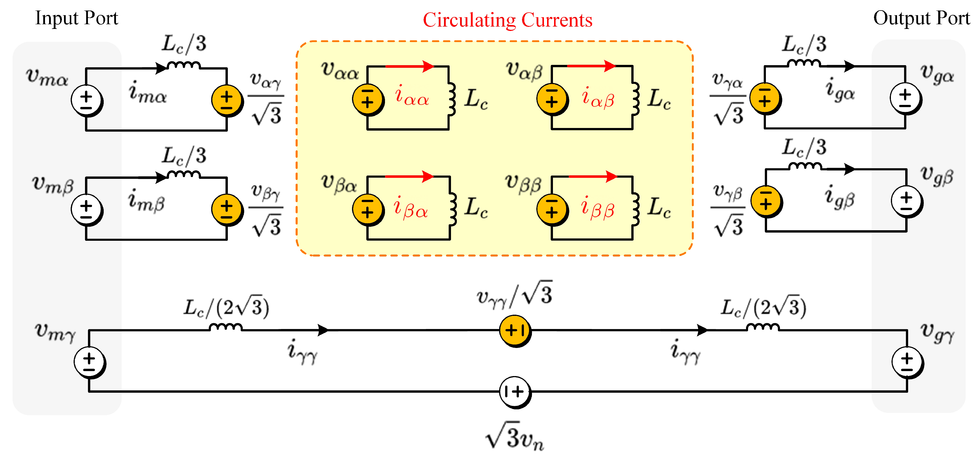
3.1.3. Circulating Current Identification

The Circulating currents model is used to identify the number of available independent inner current paths of the $M^{3}C$. Starting from the definition of output currents, it is possible to specify and clarify the feasible independent circulating currents paths of the $M^{3}C$. Using Figure 4, the input and output port currents can be defined by the following representation:

$$\left[\begin{array}{c}{i}_a\\ i_b\\ i_c\\ i_r\\ i_s\\ i_t\end{array}\right]=\underset{{\Lambda }_{\mathrm{i}}}{\underbrace{\left[\begin{array}{ccccccccc}1& 1& 1& 0& 0& 0& 0& 0& 0\\ 0& 0& 0& 1& 1& 1& 0& 0& 0\\ 0& 0& 0& 0& 0& 0& 1& 1& 1\\ 1& 0& 0& 1& 0& 0& 1& 0& 0\\ 0& 1& 0& 0& 1& 0& 0& 1& 0\\ 0& 0& 1& 0& 0& 1& 0& 0& 1\end{array}\right]}}\underset{{\mathit{i}}_{xy}}{\underbrace{\left[\begin{array}{c}{i}_{ar}\\ i_{as}\\ i_{at}\\ i_{br}\\ i_{bs}\\ i_{bt}\\ i_{cr}\\ i_{cs}\\ i_{ct}\end{array}\right]}}$$

(15)

The system in Equation (15) can be referred to the $\alpha \beta \gamma$ frame using the following expressions:

$${\mathit{T}}_{\mathit{o}}=\left[\begin{array}{cc}{\mathit{T}}_{\alpha \beta \gamma }& {\mathbf{0}}_{3\times 3}\\ {\mathbf{0}}_{3\times 3}& {\mathit{T}}_{\alpha \beta \gamma }\end{array}\right],\mathrm{with}{\mathbf{0}}_{3\times 3}=\left[\begin{array}{ccc}0& 0& 0\\ 0& 0& 0\\ 0& 0& 0\end{array}\right]\mathrm{and}{\mathit{T}}_{\alpha \beta \gamma }=\frac{1}{\sqrt{6}}\left[\begin{array}{ccc}2& -1& -1\\ 0& \sqrt{3}& -\sqrt{3}\\ \sqrt{2}& \sqrt{2}& \sqrt{2}\end{array}\right]$$

(16)

Therefore, if Equation (15) is premultiplied by ${\mathit{T}}_o$, the output currents are represented in the $\alpha \beta \gamma$ frame. As mentioned in [40], the zero sequence component at both ports is neglected because the neutral output points are galvanically isolated. Using this consideration, the next matrix transform can be defined:

$$\left[\begin{array}{c}{i}_{m\alpha }\\ i_{m\beta }\\ i_{g\alpha }\\ i_{g\beta }\\ i_{\gamma \gamma }\end{array}\right]=\frac{1}{\sqrt{6}}\left[\begin{array}{ccccccccc}2& 2& 2& -1& -1& -1& -1& -1& -1\\ 0& 0& 0& \sqrt{3}& \sqrt{3}& \sqrt{3}& -\sqrt{3}& -\sqrt{3}& -\sqrt{3}\\ 2& -1& -1& 2& -1& -1& 2& -1& -1\\ 0& \sqrt{3}& -\sqrt{3}& 0& \sqrt{3}& -\sqrt{3}& 0& \sqrt{3}& -\sqrt{3}\\ \sqrt{2}& \sqrt{2}& \sqrt{2}& \sqrt{2}& \sqrt{2}& \sqrt{2}& \sqrt{2}& \sqrt{2}& \sqrt{2}\end{array}\right]{\mathit{i}}_{xy}$$

(17)

According to [15,40], the dimension of the null space of matrix ${\Lambda }_{\mathrm{i}}$ defines the number of circulating currents available in the converter. In the case of the $M^{3}C$, the null space of the system is four ($\dim \left\{\mathrm{nullity}\left({\Lambda }_{\mathrm{i}}\right)\right\}=4$), and consequently, the number of circulating currents is four when the $M^{3}C$ operates under nominal conditions with its nine clusters.

It is worth to mention that, many circulating current paths can be defined for the $M^{3}C$ as long as the linear combination of the cluster currents belongs to the null space of ${\Lambda }_{\mathrm{i}}$. However, the Double$-\alpha \beta \gamma$ and the $\Sigma \Delta$ frames are the most utilised transforms [24,41].

3.2. Double$-\alpha \beta \gamma$ Frame Modelling

This modelling approach is based on the identification of the circulating currents of the converter using a linear transformation referred to as Double$-\alpha \beta \gamma$ Transformation. This was partially introduced in [41], and fully proposed and analysed in [42].

The Double$-\alpha \beta \gamma$ transformation is based on the Clarke Transformation, and it is used to decouple the input, output and $M^{3}C$ voltages and currents. This modelling comprises a Voltage-Current Model and a Power-Capacitor Voltage Model of the $M^{3}C$.

3.2.1. Voltage-Current Model of the $M^{3}C$

The Double$-\alpha \beta \gamma$ transformation is obtained by pre-multiplying Equation (9) by ${\mathit{T}}_{\alpha \beta \gamma }^T$, and post-multiplying it by ${\mathit{T}}_{\alpha \beta \gamma }$ [24,42]. The matrix ${\mathit{T}}_{\alpha \beta \gamma }$ is defined in Equation (16). Thus, the resulting system is named the Voltage-Current model of the $M^{3}C$ in Double$-\alpha \beta \gamma$ frame:

$$\begin{array}{cc}\hfill \sqrt{3}\left[\begin{array}{ccc}0& 0& 0\\ 0& 0& 0\\ v_{m\alpha }& v_{m\beta }& v_{m\gamma }\end{array}\right]& =L_c\frac{d}{dt}\left[\begin{array}{ccc}{i}_{\alpha \alpha }& i_{\beta \alpha }& i_{\gamma \alpha }\\ i_{\alpha \beta }& i_{\beta \beta }& i_{\gamma \beta }\\ i_{\alpha \gamma }& i_{\beta \gamma }& i_{\gamma \gamma }\end{array}\right]+\left[\begin{array}{ccc}{v}_{\alpha \alpha }& v_{\beta \alpha }& v_{\gamma \alpha }\\ v_{\alpha \beta }& v_{\beta \beta }& v_{\gamma \beta }\\ v_{\alpha \gamma }& v_{\beta \gamma }& v_{\gamma \gamma }\end{array}\right]+\sqrt{3}\left[\begin{array}{ccc}0& 0& v_{g\alpha }\\ 0& 0& v_{g\beta }\\ 0& 0& v_{g\gamma }\end{array}\right]+\left[\begin{array}{ccc}0& 0& 0\\ 0& 0& 0\\ 0& 0& 3v_n\end{array}\right]\hfill \end{array}$$

(18)

One of the principal benefits of using the Double$-\alpha \beta \gamma$ transformation for the $M^{3}C$ is obtaining a decoupled representation for the input port, output port and circulating currents [41]. To highlight this feature, the Voltage-Current model of Equation (18) is expressed as follows:

$$\begin{array}{cc}\hfill \sqrt{3}\left[\begin{array}{c}{v}_{m\alpha }\\ v_{m\beta }\end{array}\right]& =\left[\begin{array}{c}{v}_{\alpha \gamma }\\ v_{\beta \gamma }\end{array}\right]+L_c\frac{d}{dt}\left[\begin{array}{c}{i}_{\alpha \gamma }\\ i_{\beta \gamma }\end{array}\right]\hfill \end{array}$$

(19)

$$\begin{array}{cc}\hfill -\sqrt{3}\left[\begin{array}{c}{v}_{g\alpha }\\ v_{g\beta }\end{array}\right]& =\left[\begin{array}{c}{v}_{\gamma \alpha }\\ v_{\gamma \beta }\end{array}\right]+L_c\frac{d}{dt}\left[\begin{array}{c}{i}_{\gamma \alpha }\\ i_{\gamma \beta }\end{array}\right]\hfill \end{array}$$

(20)

$$\begin{array}{cc}\hfill \left[\begin{array}{cc}{v}_{\alpha \alpha }& v_{\beta \alpha }\\ v_{\alpha \beta }& v_{\beta \beta }\end{array}\right]& =-L_c\frac{d}{dt}\left[\begin{array}{cc}{i}_{\alpha \alpha }& i_{\beta \alpha }\\ i_{\alpha \beta }& i_{\beta \beta }\end{array}\right]\hfill \end{array}$$

(21)

$$\begin{array}{cc}\hfill \sqrt{3}{v}_{m\gamma }& =L_c\frac{d}{dt}{i}_{\gamma \gamma }+v_{\gamma \gamma }+\sqrt{3}{v}_{g\gamma }+3v_n\hfill \end{array}$$

(22)

To further simplify the model, the input and output port currents can be represented as a function of the transformed currents [42]. Then, the following expressions can be derived from Equation (18):

$$\begin{array}{c}\hfill i_{m\alpha }=\sqrt{3}{i}_{\alpha \gamma };i_{m\beta }=\sqrt{3}{i}_{\beta \gamma }\end{array}$$

(23)

$$\begin{array}{c}\hfill i_{g\alpha }=\sqrt{3}{i}_{\gamma \alpha };i_{g\beta }=\sqrt{3}{i}_{\gamma \beta }\end{array}$$

(24)

At this stage, it is possible to replace Equations (23) and (24) into Equations (19) and (20), obtaining the equivalent circuits presented in Figure 5. The currents and voltages of the input-port are represented in Equation (19), and the output-port variables are described in Equation (20). The transformed cluster voltages and currents of the $M^{3}C$ are represented by Equation (21) and the common-mode voltage Equation (22). The currents $i_{\alpha \alpha }$, $i_{\beta \alpha }$, $i_{\alpha \beta }$ and $i_{\beta \beta }$ are referred to as circulating currents in the Double$-\alpha \beta \gamma$ frame due to the fact that they are not reflected at the input or output ports.

The common-mode model in Equation (22) can be simplified to $v_{\gamma \gamma }=-3v_n$ when the input and output port voltages are balanced (i.e., $v_{g\gamma }=v_{m\gamma }=0$), and the neutral points of the input and output are galvanically isolated (i.e., $i_{\gamma \gamma }=0$).

3.2.2. Power-CCV Model

As proposed in [24,41], the Double$-\alpha \beta \gamma$ Transformation can be also applied to the Power-Capacitor Voltage Model of the $M^{3}C$ model (see Equation (13)) to enable a decoupled representation of the energy interactions in the $M^{3}C$. Consequently, Equation (13) is pre-multiplied by ${\mathit{T}}_{\alpha \beta \gamma }^T$ and post-multiplied by ${\mathit{T}}_{\alpha \beta \gamma }$ to obtain:

$$\begin{array}{c}\hfill C{v}_C^{*}\frac{d}{dt}\left[\begin{array}{ccc}{v}_{C\alpha \alpha }& v_{C\beta \alpha }& v_{C\gamma \alpha }\\ v_{C\alpha \beta }& v_{C\beta \beta }& v_{C\gamma \beta }\\ v_{C\alpha \gamma }& v_{C\beta \gamma }& v_{C\gamma \gamma }\end{array}\right]\approx \left[\begin{array}{ccc}{P}_{\alpha \alpha }& P_{\beta \alpha }& P_{\gamma \alpha }\\ P_{\alpha \beta }& P_{\beta \beta }& P_{\gamma \beta }\\ P_{\alpha \gamma }& P_{\beta \gamma }& P_{\gamma \gamma }\end{array}\right]\end{array}$$

(25)

Equation (25) defines the Power-Capacitor Voltage Model of the $M^{3}C$ in Double$-\alpha \beta \gamma$ frame. The power components of the right-hand of Equation (25) can be represented as a function of the transformed voltages and currents of the $M^{3}C$ in Double-$\alpha \beta \gamma$ coordinates [24]. Thus, the Double$-\alpha \beta \gamma$ transformation is also applied to Equation (14), yielding to:

$$P_{\alpha \alpha }=\frac{1}{3}(v_{m\alpha }{i}_{g\alpha }-v_{g\alpha }{i}_{m\alpha })+\frac{1}{\sqrt{6}}(v_{m\alpha }{i}_{\alpha \alpha }-v_{m\beta }{i}_{\beta \alpha })-\frac{1}{\sqrt{6}}(v_{g\alpha }{i}_{\alpha \alpha }-v_{g\beta }{i}_{\alpha })-v_n{i}_{\alpha \alpha }$$

(26)

$$P_{\alpha \beta }=\frac{1}{3}(v_{m\alpha }{i}_{g\beta }-v_{g\beta }{i}_{m\alpha })+\frac{1}{\sqrt{6}}(v_{m\alpha }{i}_{\alpha \beta }-v_{m\beta }{i}_{\beta \beta })+\frac{1}{\sqrt{6}}(v_{g\alpha }{i}_{\alpha \beta }+v_{g\beta }{i}_{\alpha \alpha })-v_n{i}_{\alpha \beta }$$

(27)

$$P_{\beta \alpha }=\frac{1}{3}(v_{m\beta }{i}_{g\alpha }-v_{g\alpha }{i}_{m\beta })-\frac{1}{\sqrt{6}}(v_{m\alpha }{i}_{\beta \alpha }+v_{m\beta }{i}_{\alpha \alpha })-\frac{1}{\sqrt{6}}(v_{g\alpha }{i}_{\beta \alpha }-v_{g\beta }{i}_{\beta \beta })-v_n{i}_{\beta \alpha }$$

(28)

$$P_{\beta \beta }=\frac{1}{3}(v_{m\beta }{i}_{g\beta }-v_{g\beta }{i}_{m\beta })-\frac{1}{\sqrt{6}}(v_{m\alpha }{i}_{\beta \beta }+v_{m\beta }{i}_{\alpha \beta })+\frac{1}{\sqrt{6}}(v_{g\alpha }{i}_{\beta \beta }+v_{g\beta }{i}_{\beta \alpha })-v_n{i}_{\beta \beta }$$

(29)

$$P_{\alpha \gamma }=\phantom{-}\frac{1}{3\sqrt{2}}(v_{m\alpha }{i}_{m\alpha }-v_{m\beta }{i}_{m\beta })-\frac{1}{\sqrt{3}}(v_{g\alpha }{i}_{\alpha \alpha }+v_{g\beta }{i}_{\alpha \beta })-\frac{1}{\sqrt{3}}{v}_n{i}_{m\alpha }$$

(30)

$$P_{\beta \gamma }=-\frac{1}{3\sqrt{2}}(v_{m\alpha }{i}_{m\beta }+v_{m\beta }{i}_{m\alpha })-\frac{1}{\sqrt{3}}(v_{g\alpha }{i}_{\beta \alpha }+v_{g\beta }{i}_{\beta \beta })-\frac{1}{\sqrt{3}}{v}_n{i}_{m\beta }$$

(31)

$$P_{\gamma \alpha }=-\frac{1}{3\sqrt{2}}(v_{g\alpha }{i}_{g\alpha }-v_{g\beta }{i}_{g\beta })+\frac{1}{\sqrt{3}}(v_{m\alpha }{i}_{\alpha \alpha }+v_{m\beta }{i}_{\beta \alpha })-\frac{1}{\sqrt{3}}{v}_n{i}_{g\alpha }$$

(32)

$$P_{\gamma \beta }=\phantom{-}\frac{1}{3\sqrt{2}}(v_{g\alpha }{i}_{g\beta }+v_{g\beta }{i}_{g\alpha })+\frac{1}{\sqrt{3}}(v_{m\alpha }{i}_{\alpha \beta }+v_{m\beta }{i}_{\beta \beta })-\frac{1}{\sqrt{3}}{v}_n{i}_{g\beta }$$

(33)

$$P_{\gamma \gamma }=\phantom{-}\frac{1}{3}(v_{m\alpha }{i}_{m\alpha }+v_{m\beta }{i}_{m\beta })-\frac{1}{3}(v_{g\alpha }{i}_{g\alpha }+v_{g\beta }{i}_{g\beta })$$

(34)

The power components given in Equations (26)–(34) represent the energy changes in the $M^{3}C$, and they define the CCV oscillations of the left side of Equation (25). From a physical point of view, the CCV oscillations have the following meaning [13,31]:

• $v_{C\alpha \alpha }$, $v_{C\beta \alpha }$, $v_{C\alpha \beta }$, $v_{C\beta \beta }$ represent CCV imbalances among clusters inside the same Sub-Converter. They are referred to as Intra-CCV Imbalance terms in [27], and as Inner Imbalance terms in [24]. These components have a dominant voltage oscillation of frequencies $f_m\pm f_g$.
• $v_{C\gamma \alpha }$, $v_{C\gamma \beta }$, $v_{C\alpha \gamma }$ and $v_{C\beta \gamma }$ represent CCV imbalances among clusters of different Sub-Converters. They are referred to as Inter-CCV Imbalance terms in [24,27]. The terms $v_{C\gamma \alpha }$ and $v_{C\gamma \beta }$ have a dominant voltage oscillation of frequency $2f_g$, whereas $v_{C\alpha \gamma }$ and $v_{C\beta \gamma }$ have a dominant voltage oscillation of frequency $2f_m$.
• $v_{C\gamma \gamma }$ is linked to the total active power being injected/consumed for the $M^{3}C$. It can be used to impose the average value of all the CCVs.

All the floating capacitor voltages must be controlled to the same voltage reference to obtain correct operation of the $M^{3}C$. When this condition is fulfilled, for instance all the capacitor voltages are equal to $v_c^{*}$, the power flows of Equations (26)−(34) tend to zero, and Equation (25) yields to [24,27]:

$$\begin{array}{c}\hfill \left[\begin{array}{ccc}{v}_{C\alpha \alpha }& v_{C\beta \alpha }& v_{C\gamma \alpha }\\ v_{C\alpha \beta }& v_{C\beta \beta }& v_{C\gamma \beta }\\ v_{C\alpha \gamma }& v_{C\beta \gamma }& v_{C\gamma \gamma }\end{array}\right]\approx \left[\begin{array}{ccc}0& 0& 0\\ 0& 0& 0\\ 0& 0& 3n{v}_C^{*}\end{array}\right]\end{array}$$

(35)

3.3. $\Sigma \Delta$ Frame Modelling

An extra linear transformation, referred to as $\Sigma \Delta$ transformation, has been proposed to obtain a geometrical orientation of the four circulating currents of the $M^{3}C$ [43]. This transformation has also been used in $M^{2}C$ applications, focusing on the interaction of the electrical variables among the converter upper and lower clusters [25,44,45].

The $\Sigma \Delta$ transformation is represented as follows:

$$\begin{array}{c}\hfill \left[\begin{array}{c}{X}_{1\alpha }^{\Sigma \Delta }\\ X_{1\beta }^{\Sigma \Delta }\\ X_{2\alpha }^{\Sigma \Delta }\\ X_{2\beta }^{\Sigma \Delta }\end{array}\right]=\frac{1}{2}\left[\begin{array}{cccc}1& 0& \hfill 0& \hfill 1\\ 0& 1& \hfill -1& \hfill 0\\ 1& 0& \hfill 0& \hfill -1\\ 0& 1& \hfill 1& \hfill 0\end{array}\right]\left[\begin{array}{c}{X}_{\alpha \alpha }\\ X_{\alpha \beta }\\ X_{\beta \alpha }\\ X_{\beta \beta }\end{array}\right]\end{array}$$

(36)

Similarly, the $\Sigma \Delta$ transformation is used over the terms $v_{C\alpha \alpha }$, $v_{C\alpha \beta }$, $v_{C\beta \alpha }$ and $v_{C\beta \beta }$. Then, is possible to express Equation (25) in $\Sigma \Delta$ Double$-\alpha \beta \gamma$ as follows:

$$\begin{array}{c}\hfill C{v}_C^{*}\frac{d}{dt}\left[\begin{array}{ccc}{v}_{C1\alpha }^{\Sigma \Delta }& v_{C1\beta }^{\Sigma \Delta }& v_{C\gamma \alpha }^{}\\ v_{C2\alpha }^{\Sigma \Delta }& v_{C2\beta }^{\Sigma \Delta }& v_{C\gamma \beta }^{}\\ v_{C\alpha \gamma }^{}& v_{C\beta \gamma }^{}& v_{C\gamma \gamma }^{}\end{array}\right]\approx \left[\begin{array}{ccc}{P}_{1\alpha }^{\Sigma \Delta }& P_{1\beta }^{\Sigma \Delta }& P_{\gamma \alpha }\\ P_{2\alpha }^{\Sigma \Delta }& P_{2\beta }^{\Sigma \Delta }& P_{\gamma \beta }\\ P_{\alpha \gamma }& P_{\beta \gamma }& P_{\gamma \gamma }\end{array}\right]\end{array}$$

(37)

Thus, the new power-terms on the right-hand side of Equation (37) can also be expressed as a function of the transformed currents and voltages of the converter as follows:

$$P_{1\alpha }^{\Sigma \Delta }=\frac{1}{6}\left[(v_{m\alpha }{i}_{g\alpha }-v_{g\alpha }{i}_{m\alpha })+(v_{m\beta }{i}_{g\beta }-v_{g\beta }{i}_{m\beta })\right]+\frac{1}{\sqrt{6}}\left[(v_{m\alpha }{i}_{2\alpha }^{\Sigma \Delta }-v_{m\beta }{i}_{2\beta }^{\Sigma \Delta })+(-v_{g\alpha }{i}_{2\alpha }^{\Sigma \Delta }+v_{g\beta }{i}_{2\beta }^{\Sigma \Delta })\right]-v_n{i}_{1\alpha }^{\Sigma \Delta }$$

(38)

$$P_{1\beta }^{\Sigma \Delta }=\frac{1}{6}\left[(v_{m\alpha }{i}_{g\beta }-v_{g\beta }{i}_{m\alpha })-(v_{m\beta }{i}_{g\alpha }-v_{g\alpha }{i}_{m\beta })\right]+\frac{1}{\sqrt{6}}\left[(v_{m\alpha }{i}_{2\beta }^{\Sigma \Delta }+v_{m\beta }{i}_{2\alpha }^{\Sigma \Delta })+(v_{g\alpha }{i}_{2\beta }^{\Sigma \Delta }+v_{g\beta }{i}_{2\alpha }^{\Sigma \Delta })\right]-v_n{i}_{1\beta }^{\Sigma \Delta }$$

(39)

$$P_{2\alpha }^{\Sigma \Delta }=\frac{1}{6}\left[(v_{m\beta }{i}_{g\alpha }-v_{g\alpha }{i}_{m\beta })-(v_{m\beta }{i}_{g\beta }-v_{g\beta }{i}_{m\beta })\right]+\frac{1}{\sqrt{6}}\left[(v_{m\alpha }{i}_{1\alpha }^{\Sigma \Delta }+v_{m\beta }{i}_{1\beta }^{\Sigma \Delta })+(-v_{g\alpha }{i}_{1\alpha }^{\Sigma \Delta }+v_{g\beta }{i}_{1\beta }^{\Sigma \Delta })\right]-v_n{i}_{2\alpha }^{\Sigma \Delta }$$

(40)

$$P_{2\beta }^{\Sigma \Delta }=\frac{1}{6}\left[(v_{m\beta }{i}_{g\beta }-v_{g\beta }{i}_{m\beta })+(v_{m\beta }{i}_{g\alpha }-v_{g\alpha }{i}_{m\beta })\right]+\frac{1}{\sqrt{6}}\left[(v_{m\alpha }{i}_{1\beta }^{\Sigma \Delta }-v_{m\beta }{i}_{1\alpha }^{\Sigma \Delta })+(v_{g\alpha }{i}_{1\beta }^{\Sigma \Delta }+v_{g\beta }{i}_{1\alpha }^{\Sigma \Delta })\right]-v_n{i}_{2\beta }^{\Sigma \Delta }$$

(41)

$$P_{\alpha \gamma }=\frac{1}{3\sqrt{2}}\left[(v_{m\alpha }{i}_{m\alpha }-v_{m\beta }{i}_{m\beta })\right]-\frac{1}{\sqrt{3}}\left[v_{g\alpha }(i_{1\alpha }^{\Sigma \Delta }+i_{2\alpha }^{\Sigma \Delta })+v_{g\beta }(i_{1\beta }^{\Sigma \Delta }+i_{2\beta }^{\Sigma \Delta })-v_n{i}_{m\alpha }\right]$$

(42)

$$P_{\beta \gamma }=-\frac{1}{3\sqrt{2}}\left[(v_{m\alpha }{i}_{m\beta }+v_{m\beta }{i}_{m\alpha })\right]-\frac{1}{\sqrt{3}}\left[v_{g\alpha }(-i_{1\beta }^{\Sigma \Delta }+i_{2\beta }^{\Sigma \Delta })+v_{g\beta }(i_{1\alpha }^{\Sigma \Delta }-i_{2\alpha }^{\Sigma \Delta })-v_n{i}_{m\beta }\right]$$

(43)

$$P_{\gamma \alpha }=-\frac{1}{3\sqrt{2}}\left[(v_{g\alpha }{i}_{g\alpha }-v_{g\beta }{i}_{g\beta })\right]+\frac{1}{\sqrt{3}}\left[v_{m\alpha }(i_{1\alpha }^{\Sigma \Delta }+i_{2\alpha }^{\Sigma \Delta })+v_{m\beta }(-i_{1\beta }^{\Sigma \Delta }+i_{2\beta }^{\Sigma \Delta })-v_n{i}_{g\alpha }\right]$$

(44)

$$P_{\gamma \beta }=\frac{1}{3\sqrt{2}}\left[(v_{g\alpha }{i}_{g\beta }+v_{g\beta }{i}_{g\alpha })\right]+\frac{1}{\sqrt{3}}\left[v_{m\alpha }(i_{1\beta }^{\Sigma \Delta }+i_{2\beta }^{\Sigma \Delta })+v_{m\beta }(i_{1\alpha }^{\Sigma \Delta }-i_{2\alpha }^{\Sigma \Delta })-v_n{i}_{g\beta }\right]$$

(45)

3.4. Vector Power-CCV Modelling

The vector representation of the Power-CCV model of the $M^{3}C$ has been proposed in [32,46,47]. The first step is to use vector notation for the cluster capacitor voltages and powers in Equations (38)–(41), as follows:

$${\mathit{P}}_{1\alpha \beta }^{\Sigma \Delta }=P_{1\alpha }^{\Sigma \Delta }+j{P}_{1\beta }^{\Sigma \Delta };{\mathit{P}}_{2\alpha \beta }^{\Sigma \Delta }=P_{2\alpha }^{\Sigma \Delta }+j{P}_{2\beta }^{\Sigma \Delta }$$

(46)

$${\mathit{P}}_{\gamma }^{\alpha \beta }=P_{\alpha \gamma }+j{P}_{\beta \gamma };{\mathit{P}}_{\alpha \beta }^{\gamma }=P_{\gamma \alpha }+j{P}_{\gamma \beta }$$

(47)

$${\mathit{v}}_{C1\alpha \beta }^{\Sigma \Delta }=v_{C1\alpha }^{\Sigma \Delta }+j{v}_{C1\beta }^{\Sigma \Delta };{\mathit{v}}_{C2\alpha \beta }^{\Sigma \Delta }=v_{C2\alpha }^{\Sigma \Delta }+j{v}_{C2\beta }^{\Sigma \Delta }$$

(48)

Then, by applying the vector notation to Equations (38)–(45), the CCV-power model in Equation (37) can be expressed as a function of the circulating current vectors ${\mathit{i}}_{1\alpha \beta }^{\Sigma \Delta }$ and ${\mathit{i}}_{2\alpha \beta }^{\Sigma \Delta }$ as well as the common-mode voltage $v_n$ according to the following four complex-valued dynamic equations [32,46,47]:

$$C{v}_C^{*}\frac{d{\mathit{v}}_{C1\alpha \beta }^{\Sigma \Delta }}{dt}\approx {\mathit{P}}_{1\alpha \beta }^{\Sigma \Delta }=\frac{1}{6}\left({\mathit{v}}_{m_{\alpha \beta }}^c{\mathit{i}}_{g_{\alpha \beta }}-{\mathit{v}}_{g_{\alpha \beta }}{\mathit{i}}_{m_{\alpha \beta }}^c\right)+\frac{1}{\sqrt{6}}\left({\mathit{v}}_{m_{\alpha \beta }}{\mathit{i}}_{2\alpha \beta }^{\Sigma \Delta }-{\mathit{v}}_{g_{\alpha \beta }}^c{\mathit{i}}_{2\alpha \beta }^{\Sigma \Delta c}\right)-v_n{\mathit{i}}_{1\alpha \beta }^{\Sigma \Delta }$$

(49)

$$C{v}_C^{*}\frac{d{\mathit{v}}_{C2\alpha \beta }^{\Sigma \Delta }}{dt}\approx {\mathit{P}}_{2\alpha \beta }^{\Sigma \Delta }=\frac{1}{6}\left({\mathit{v}}_{m_{\alpha \beta }}{\mathit{i}}_{g_{\alpha \beta }}-{\mathit{v}}_{g_{\alpha \beta }}{\mathit{i}}_{i\alpha \beta }\right)+\frac{1}{\sqrt{6}}\left({\mathit{v}}_{m_{\alpha \beta }}^c{\mathit{i}}_{1\alpha \beta }^{\Sigma \Delta }-{\mathit{v}}_{g_{\alpha \beta }}^c{\mathit{i}}_{1\alpha \beta }^{\Sigma {\Delta }^c}\right)-v_n{\mathit{i}}_{2\alpha \beta }^{\Sigma \Delta }$$

(50)

$$C{v}_C^{*}\frac{d{\mathit{v}}_{C\gamma }^{\alpha \beta }}{dt}\approx {\mathit{P}}_{\gamma }^{\alpha \beta }=\frac{1}{3\sqrt{2}}\left({\mathit{v}}_{m_{\alpha \beta }}^c{\mathit{i}}_{m_{\alpha \beta }}^c\right)-\frac{1}{\sqrt{3}}\left({\mathit{v}}_{g_{\alpha \beta }}{\mathit{i}}_{1\alpha \beta }^{\Sigma {\Delta }^c}+{\mathit{v}}_{g_{\alpha \beta }}^c{\mathit{i}}_{2\alpha \beta }^{\Sigma \Delta }+v_n{\mathit{i}}_{m_{\alpha \beta }}\right)$$

(51)

$$C{v}_C^{*}\frac{d{\mathit{v}}_{C\alpha \beta }^{\gamma }}{dt}\approx {\mathit{P}}_{\alpha \beta }^{\gamma }=\frac{-1}{3\sqrt{2}}\left({\mathit{v}}_{g_{\alpha \beta }}^c{\mathit{i}}_{g_{\alpha \beta }}^c\right)+\frac{1}{\sqrt{3}}\left({\mathit{v}}_{m_{\alpha \beta }}{\mathit{i}}_{1\alpha \beta }^{\Sigma \Delta }+{\mathit{v}}_{m_{\alpha \beta }}^c{\mathit{i}}_{2\alpha \beta }^{\Sigma \Delta }-v_n{\mathit{i}}_{g_{\alpha \beta }}\right)$$

(52)

where:

$${\mathit{v}}_{m_{\alpha \beta }}=v_{m\alpha }+j{v}_{m\beta };{\mathit{i}}_{m_{\alpha \beta }}=i_{m\alpha }+j{i}_{m\beta }$$

(53)

$${\mathit{v}}_{g_{\alpha \beta }}=v_{g\alpha }+j{v}_{g\beta };{\mathit{i}}_{g_{\alpha \beta }}=i_{g\alpha }+j{i}_{g\beta }$$

(54)

Additionally, the superscript c stands for the complex conjugate operator. In Equations (49)–(52), the vectors ${\mathit{v}}_{m_{\alpha \beta }}$ and ${\mathit{i}}_{m_{\alpha \beta }}$ symbolise the input-port voltages and currents in the $\alpha \beta \gamma$ frame, and the vectors ${\mathit{v}}_{g_{\alpha \beta }}$ and ${\mathit{i}}_{g_{\alpha \beta }}$ represent the output-port voltages and currents in the $\alpha \beta \gamma$ frame.

Therefore, the CCV vectors ${\mathit{v}}_{C1\alpha \beta }^{\Sigma \Delta }$, ${\mathit{v}}_{C2\alpha \beta }^{\Sigma \Delta }$, ${\mathit{v}}_{C\alpha \beta }^{\gamma }$, and ${\mathit{v}}_{C\gamma }^{\alpha \beta }$ are separately related to the input–output port frequency states as follows:

• ${\mathit{v}}_{C1\alpha \beta }^{\Sigma \Delta }$ has a dominant frequency oscillation of $f_g-f_m$.
• ${\mathit{v}}_{C2\alpha \beta }^{\Sigma \Delta }$ has a dominant frequency oscillation of $f_m+f_g$.
• ${\mathit{v}}_{C\gamma }^{\alpha \beta }$ has a dominant frequency oscillation of $2f_m$.
• ${\mathit{v}}_{C\alpha \beta }^{\gamma }$ has a dominant frequency oscillation of $2f_g$.

3.5. Comparison of Modelling Approaches

At this stage, a qualitative comparison of the currently proposed modelling approaches for the $M^{3}C$ is summarised in

Table 1. Benchmarking of modelling approaches for the $M^{3}C$.

	Example	Decoupled	CCV Oscillations	Compactness	Linear Transformations
Natural Frame	[7]	No	Mixed	Low	0
Double$-\alpha \beta \gamma$	[24]	Yes	2 frequencies per CCV term	Medium	1
$\Sigma \Delta$ Double$-\alpha \beta \gamma$	[31]	Yes	1 frequencies per CCV term	Medium	2
Vector $\Sigma \Delta$ Double$-\alpha \beta \gamma$	[32]	Yes	1 frequencies per CCV term	High	2

. The comparison indicators are the capabilities of enabling a decoupled representation of the converter dynamics, the composition of the CCVs in terms of the frequency components, the compactness of the model representations, and finally, the number of linear transformations used.

As shown in Table 1, natural frame modelling is the most straightforward approach, but it fails to provide a decoupled representation of the converter. Therefore, the CCVs contain several frequency components which might result in a complex regulation. The remaining modelling approaches, i.e., Double$-\alpha \beta \gamma$, $\Sigma \Delta$ Double$-\alpha \beta \gamma$ and vector $\Sigma \Delta$ Double$-\alpha \beta \gamma$ share the common feature of allowing a decoupled $M^{3}C$ representation and identification of the circulating currents.

The main difference among Double$-\alpha \beta \gamma$ and $\Sigma \Delta$ Double$-\alpha \beta \gamma$ modelling is related to the representation of the CCVs. As shown in Table 1, the number of linear transformations used in each case is different and then the CCVs oscillations have different behaviours depending on the reference frame being used to analyse them [8,32].

As a representative example, the CCVs have been plotted in Figure 6, in per unit form, as a function of frequencies in Double$-\alpha \beta \gamma$ and $\Sigma \Delta$ frames. In this example, the input-port frequency ($f_m$) is varied from $-75$ to 75 Hz, and the output-port frequency ($f_g$) is fixed at 50 Hz, as proposed in [32]. The main differences between the reference frames analysed in this section are:

• In Double$-\alpha \beta \gamma$ frame, the CCVs, i.e., $v_{C\alpha \alpha }$, $v_{C\alpha \beta }$, $v_{C\beta \alpha }$, $v_{C\beta \beta }$, have two main oscillatory components inversely proportional to the frequencies $f_g-f_m$ and $f_g+f_m$. Therefore, the CCV presents unacceptable voltage oscillations when $f_m=f_g$ and/or $f_m=-f_g$.
• In $\Sigma \Delta$ Double$-\alpha \beta \gamma$ frame, the CCV, i.e., ${\mathit{v}}_{C1\alpha \beta }^{\Sigma \Delta }$ and ${\mathit{v}}_{C2\alpha \beta }^{\Sigma \Delta }$, have just one oscillatory component. The CCV component ${\mathit{v}}_{C1\alpha \beta }^{\Sigma \Delta }$ presents unacceptable voltage oscillations when $f_m=f_g$, and ${\mathit{v}}_{C2\alpha \beta }^{\Sigma \Delta }$ presents unacceptable voltage oscillations when $f_m=-f_g$.

Consequently, the use of the $\Sigma \Delta$ Double$-\alpha \beta \gamma$ frame facilitates the representation of the CCV oscillations in terms of the input and output port frequencies [47]. Therefore, a more straightforward filter design for the CCVs can be obtained in $\Sigma \Delta$ Double$-\alpha \beta \gamma$ due to one single frequency component requiring filtering, as stated in [31]. Finally, the vector $\Sigma \Delta$ Double$-\alpha \beta \gamma$ provides a compact representation of the CCVs in terms of the input port and output port frequencies using only four vector equations. This fact permits the use of vector control strategies to regulate the CCVs.

4. Control of the ${\mathit{M}}^{\mathbf{3}}\mathit{C}$

The $M^{3}C$ requires a suitable control strategy to achieve multiple control objectives, providing proper regulation of the input and output ports, and correct transient and steady-state regulation of the floating capacitor voltages. Therefore, most of the control approaches consider a multilayer structure composed at least of the control of the input and output currents, and the control of the $M^{3}C$.

The control of the input and output currents is generally based on standard vector control, and most of the already reported approaches focused on the control of the $M^{3}C$ [13,24,27,32,41,48].

The control of the $M^{3}C$ usually comprises CCV Control, for cluster voltage regulation, and Local Cell Balancing (LCB) Control, for power-cell voltage regulation. On the one hand, the CCV Control regulates the average value of all the floating capacitor voltages, by controlling the total energy stored in the converter [24,31]. Additionally, the CCV Control provides even energy distribution among the clusters of the converter. On the other hand, the LCB ensures proper distribution of the energy in the power-cells within a cluster. As stated in [49,50], both control loops can be considered as decoupled [49,50].

The CCV Control, the input–output port currents control, and the LCB Control are detailed in Section 4.1 and Section 4.2, Section 4.3, and Section 4.4, respectively.

4.1. Cluster Capacitor Voltage Control

The operating range of the $M^{3}C$ is divided into the DFM and the EFM to address the effect of the critical-frequency operating points on the overall control system. On the one hand, the system is considered to operate in DFM ($|f_m\pm f_g|\gg 0$). In this mode, just the average values of the floating capacitor voltages are controlled utilising the circulating currents and/or the common-mode voltage. The high-frequency oscillations in the floating capacitors are normally ignored. It is assumed that the capacitance in the power-cell is large enough to filter them out without producing a large ${\tilde{v}}_C^{}$. The control strategies proposed for this operational mode are referred to as CCV Balancing Control Strategies.

On the other hand, the $M^{3}C$ is considered to operate in EFM when $|f_m\pm f_g|$ is close or equal to zero. In this operational mode, the voltages of the floating capacitors have large low-frequency oscillations that may yield to unsafe operation of the converter. This is concluded by analysing the denominators of the third and fourth terms at the right side of Equation (7), i.e., when $f_m\approx \pm f_g$, considerable voltage oscillations might be produced. The control strategies to operate in this condition are referred to as CCV Mitigation Control Strategies, and they are based on mitigation signals, i.e., circulating currents and/or common-mode voltages as well as applying operating restrictions in the output voltage and input reactive power. The implementation of these control methodologies has been proved to successfully mitigate the large oscillations in a wide range of operational conditions [27,30,32,51].

In both modes, i.e., DFM and EFM, the CCV Control strategies use supplementary current components in the external ports and/or in the clusters as their control actions. In this subject, several control strategies have been proposed in the literature. For the sake of simplicity, this paper classifies them as:

• Control strategies based on Negative-Sequence Current Regulation (NSCR).
• Control strategies based on Circulating Current Regulation (CCR).

Using the definitions addressed above, some of the control proposals reported in the literature for the $M^{3}C$ have been summarised and categorised in

Table 2. List of $M^{3}C$ published papers sorted by type of control.

Ref.	Paper Title	Journal/Conference	CCV Control	Local Cell Balancing	Mode
[13]	A novel cascaded vector control scheme for the Modular Multilevel Matrix Converter.	IECON Proceedings	CCR	Sorting PWM	Balancing Control
[24]	Control and Experiment of a Modular Multilevel Cascade Converter Based on Triple-Star Bridge Cells	IEEE Trans. on Industry Applications	CCR	PS-PWM	Balancing Control
[27]	Control of Wind Energy Conversion Systems Based on the Modular Multilevel Matrix Converter	IEEE Trans. on Industrial Electronics	CCR	PS-PWM	Balancing Control
[30]	Experimental Verification of an Electrical Drive Fed by a Modular Multilevel TSBC Converter When the Motor Frequency Gets Closer or Equal to the Supply Frequency	IEEE Trans. on Industry Applications	CCR	PS-PWM	Mitigation Control
[31]	Energy balancing of the Modular Multilevel Matrix Converter based on a new transformed arm power analysis	EPE-ECCE	CCR	Sorting PWM	Balancing Control
[32]	Vector Control of a Modular Multilevel Matrix Converter Operating Over the Full Output-Frequency Range	IEEE Trans. on Industrial Electronics	CCR	PS-PWM	Mitigation Control
[38]	Control of a Modular Multilevel Matrix Converter for Unified Power Flow Controller Applications	Energies	CCR	PS-PWM	Mitigation Control
[41]	Fully decoupled current control and energy balancing of the Modular Multilevel Matrix Converter	EPE/PEMC	CCR	SVM	Balancing Control
[47]	Vector control strategies to enable equal frequency operation of the modular multilevel matrix converter	Journal of Engineering	CCR	PS-PWM	Mitigation Control
[48]	A Branch Current Reallocation Based Energy Balancing Strategy for the Modular Multilevel Matrix Converter Operating Around Equal Frequency	IEEE Trans. on Power Electronics	CCR	PWM	Balancing Control
[52]	A Low-Speed, High-Torque Motor Drive Using a Modular Multilevel Cascade Converter Based on Triple-Star Bridge Cells (MMCC-TSBC)	IEEE Trans. on Industry Applications	CCR	PS-PWM	Mitigation Control
[53]	A Broad Range of Speed Control of a Permanent Magnet Synchronous Motor Driven by a Modular Multilevel TSBC Converter	IEEE Trans. on Industry Applications	CCR	PS-PWM	Mitigation Control
[54]	A new family of matrix converters for Wind Power Applications.	IECON Proceedings	CCR	SVM	Balancing Control
[57]	An Optimal Full Frequency Control Strategy for the Modular Multilevel Matrix Converter Based on Predictive Control	IEEE Trans. on Power Electronics	CCR	PS-PWM	Balancing Control
[58]	Control of a Modular Multilevel Matrix Converter for High Power Applications	Studies in Informatics and Control	NSCR	PS-PWM	Balancing Control
[59]	Independent Control of Input Current, Output Voltage, and Capacitor Voltage Balancing for a Modular Matrix Converter	IEEE Trans. on Industry Applications	NSCR	PS-PWM	Balancing Control
[60]	Benefits of operating Doubly Fed Induction Generators by Modular Multilevel Matrix Converters	PCIM Europe Conference Proceedings	CCR	Sorting PWM	Balancing Control
[61]	Optimized Branch Current Control of Modular Multilevel Matrix Converters under Branch Fault Conditions	IEEE Trans. on Power Electronics	CCR	PS-PWM	Balancing Control
[62]	Distributed Control for the Modular Multilevel Matrix Converter	IEEE Trans. on Power Electronics	CCR	PS-PWM	Balancing Control

. This classification considers CCV Control, LCB Control and operational modes. The CCV control is categorised as NSCR or CCR. The LCB control methods are divided into Phase-Shifted (PS) Pulse Wide Modulation (PWM) (e.g., [52,53]), Level Shifted (LS) PWM (e.g., [43,51]), Space Vector Modulation (e.g., [54,55,56] and Predictive Control (e.g., [50,57]). Finally, the operating mode can be Balancing Control or Mitigation Control. Most of the currently proposed $M^{3}C$ based control strategies are based on CCR and are designed for Balancing Control as verified in Table 2. Consequently, the next subsections are focusing on detailing and comparing CCV Balancing Control Strategies based on NSCR and CCR. Thereafter, CCV Mitigation Control is analysed in Section 4.5.

4.1.1. Control Strategies Based on Negative-Sequence Current Regulation

An intuitive control approach for regulating the imbalance among the floating capacitor voltages is the utilisation of NSCR. This strategy can be easily implemented in the natural $a-b-c$ frame. In general, NSCR-based balancing nested control loops are utilised, with an internal cluster current control system and an external control loop for CCV Balancing Control [58,59,63].

The imbalances among floating capacitor voltages are regulated by injecting unbalanced input or output port currents. Then, an active power component flows among different clusters to balance the capacitor voltages. Although the NCSR is a simple and straightforward strategy, the regulation of the converter is not entirely decoupled, and the control of the floating capacitor voltages affect either the input or the output ports [35,54,55,58,59,63,64,65]. It is important to mention that all these papers have considered DFM operation of the $M^{3}C$ only. The feasibility of EFM operation of the $M^{3}C$ using NSCR has not been studied yet.

NSCR proposals are based on previously reported control schemes for Cascade H-Bridge STATCOMs [4,66,67]. Balancing is usually achieved by considering the $M^{3}C$ as three sub-converters, where the neutral points of the sub-converters provide a connection to derive the output port current. Notice that this output current is homopolar in the three clusters of the subconverter. Then, the output current can be represented as a zero-sequence current in a particular subconverter [58].

As a representative example, the control strategy discussed in [58] is presented in Figure 7. Notice that this control system is used to balance only one subconverter of the three utilised in a typical $M^{3}C$ (see Figure 2a). The CCV in each sub-converter is transformed to $\alpha \beta \gamma$. The resulting components, namely $u_{\alpha }$, $u_{\beta }$, $u_{\gamma }$ are regulated with PI controllers manipulating the cluster currents. The components $u_{\alpha }$ and $u_{\beta }$ are regulated to 0 because they represent capacitor voltage imbalance, whereas the component $u_{\gamma }$ is controlled to maintain the total energy of the cluster in a constant value.

At the output of the $u_{\alpha }$ and $u_{\beta }$ controller, a negative-sequence current reference in phase with the input port voltage is obtained. Additionally, the output of the $u_{\gamma }$ PI regulator is a positive-sequence current reference component in phase with the input-port voltage. The resultant signals are used as cluster current reference signals considering the addition of 1/3 of the output current (i.e., zero-sequence current reference in the subconverter) to obtain $i_{ay}^{*}$ and $i_{by}^{*}$. Finally, in the inner loop, dead-beat controllers are used to track the arm current references.

Once the cluster voltage reference is obtained, other control loops are used for the Local Cell Balancing as discussed in Section 4.4. Besides Local Cell Balancing, the modulation technique used in [58], and also used in [59,63] is based on Phase-Shifted Pulse Wide Modulation (PS-PWM). In other works, such as [54,55,64], control strategies based on Space Vector Modulation have also been applied to synthesise the cluster voltage references of the $M^{3}C$. However, Space Vector Modulation is hardly achievable for more than two power-cells because of the massive number of potential vectors ($3^{9n}$ possible switching states for an $M^{3}C$ with n cells per cluster) [27]. Furthermore, CCV Mitigation Control of the $M^{3}C$ is not considered in [35,54,55,58,59,63,64,65].

4.1.2. Control Strategies Based on Circulating Current Regulation

The control strategies using CCR share the common feature of being fully decoupled. Then, the input and output ports currents and voltages are not affected by the regulation of the floating capacitors and vice versa. Typically, CCR based strategies consider regulations schemes for the input port currents, output port currents, circulating currents, overall energy of the converter, and the floating capacitor voltages.

CCR strategies are typically performed in either Double$-\alpha \beta \gamma$ or $\Sigma \Delta$ Double$-\alpha \beta \gamma$ frames. Most of the papers using CCR are based on the decoupled models of the $M^{3}C$ in Double$-\alpha \beta \gamma$, which are discussed in Equations (18) and (25) and illustrated in Figure 5 [8,10,13,24,28,29,30,41,48,52,53,57,61,68]. Additionally, other research proposals use the $\Sigma \Delta$ Double$-\alpha \beta \gamma$ frame as discussed in Equations (37) and (38) [32,38,41,43,46,47].

Both methodologies, i.e., based in Double$-\alpha \beta \gamma$ and $\Sigma \Delta$ Double$-\alpha \beta \gamma$, can perform either CCV Balancing Control or CCV Mitigation Control. CCV Balancing Control usually neglects the relatively high-frequency power oscillations in the CCVs, for instance, the 100 Hz produced by $2{\omega }_g$ in Equation (7), which do not produce large voltage oscillations in the capacitors considering the relatively large capacitance of the cells. However, as aforementioned, the low-frequency drift in the capacitor voltages produced by the nonlinearities and non-idealities in the power converter has to be regulated using circulating currents.

Figure 8 shows a simplified scheme for the control of the $M^{3}C$ using the CCR strategy reported in [24] (based on Double$-\alpha \beta \gamma$). This control strategy is comprised of a nested control structure for the CCV Balancing Control and CCR, allowing independent regulation of the input and output port currents as presented in Equations (19) and (20). The research group of [24] have also published similar control strategies for STATCOM applications [4], synchronous motors fed by an $M^{3}C$ [53], induction motors fed by $M^{3}C$s [29,37,68] among other works.

The control of the $M^{3}C$ is also carried out in the $\Sigma \Delta$ Double$-\alpha \beta \gamma$ frame as proposed in [32,41]. The principal distinction relies on the CCR that is performed in the $\Sigma \Delta$ frame. Then, the circulating currents are transformed from Double$-\alpha \beta \gamma$ to $\Sigma \Delta$ using Equation (36). These linear transformations make the analysis more straightforward, and it also facilitates the management of the circulating currents and common-mode voltage as degrees of freedom.

4.1.3. NSCR and CCR Comparison

NSCR and CCR control approaches have been validated for different applications, as depicted and categorised previously in Table 2. Nevertheless, there are important performance indicators that must be taken into consideration before choosing a control approach for a defined application. Consequently, a qualitative comparison of the NSCR and CCR approaches is presented in

Table 3. Comparison of Negative-Sequence Current Regulation (NSCR) and CCR control strategies.

Control Loop	Type		Advantage	Disadvantage	DFM	EFM
CCV Balancing Control	NSCR		Simple	Negative-sequence currents in the grid	Adequate	No
	CCR	Double$-\alpha \beta \gamma$	Decoupled CCV Control	Complexity	Excellent	Good
	CCR	$\Sigma \Delta$ Double$-\alpha \beta \gamma$	Decoupled CCV Control	Complexity	Excellent	Excellent

. The comparison indicators are based on the advantages and disadvantages of each method, besides qualitative performance indicators for DFM and EFM.

As depicted in Table 3, NSCR has the advantage of simple implementation, but it lacks a decoupled regulation of the $M^{3}C$. This means that the negative-sequence current must be injected at the port of the converter to ensure CCV Control. Additionally, the EFM operation of the $M^{3}C$ using NSCR has not been validated yet (see Table 2), probably because of the high magnitude of unbalanced currents required at the converter ports.

On the other hand, CCR based control strategies require a more complicated implementation using 1 or 2 linear transformation (see Table 1). Nevertheless, this could be realised considering the capabilities of modern control platforms and successful experimental validations have been presented in the literature. CCR control has been proven to be an effective solution for either DFM and EFM operation. In general, the operation using CCR is superior to the one obtained using NSCR [27,31] due to the use of the circulating currents and common-mode voltage as degrees of freedom to regulate the CVVs, and then negative sequence current is avoided.

Consequently, the next subsections are focused on a discussion of CCV Control based on CCR. Firstly, a revision of CCV Balancing Control Strategies. Then, CCV Mitigation Control Strategies are discussed in Section 4.5.

4.2. CCV Control Based on CCR

As is reported in the literature [13,24,27,32,41,48], this approaches $M^{3}C$ usually consider Average Capacitor Voltage (ACV) Control, and CCV Balancing Control as described in the next sections.

4.2.1. Average Capacitor Voltage Control

The main goal of the ACV Control is to regulate the average value of all the floating capacitor voltages at a specified voltage level.

Most of the reported strategies achieve the average capacitor voltage target by regulating the transformed term $v_{C\gamma \gamma }$ in Equation (55) at its desired reference value $3n{v}_C^{*}$. In this regard, from the Power-CCV modelling shown in Equations (34) and (37), the dynamic behaviour of $v_{C\gamma \gamma }$ is related with input and output power ports as follows:

$$C{v}_C^{*}\frac{d{v}_{C\gamma \gamma }^{}}{dt}\approx P_{\gamma \gamma }=\frac{1}{3}{p}_{in}-\frac{1}{3}{p}_{out}$$

(55)

where $p_{in}=v_{m\alpha }{i}_{m\alpha }+v_{m\beta }{i}_{m\beta }$ represents the power supplied to the $M^{3}C$ from the input port. Additionally, $p_{out}=v_{g\alpha }{i}_{g\alpha }+v_{g\beta }{i}_{g\beta }$ is the power supplied by the $M^{3}C$ to the output port where a load as an induction machine can be fed.

From a control perspective, in Equation (55), $p_{in}$ can be viewed as the manipulated variable, and $p_{out}$ could be considered as an external disturbance, which can be feedforwarded to the control system [24]. Depending on the application, the signal $p_{in}$ could be utilised to obtain a torque reference signal for an electrical machine or the power current component reference when a grid is connected at the input port terminals [41]. For instance the $v_{C\gamma \gamma }$ control scheme could be based on a Proportional-Integral (PI) controller providing the reference for the magnitude of the input port power current control [24,27].

4.2.2. CCV Balancing Control:

The CCV Balancing Control aims to distribute the energy stored in the $M^{3}C$ evenly among the different clusters. In Figure 9 the detailed control diagram for a CCV Balancing Control is presented. In this case, the control diagram is proposed in [24,27].

The $M^{3}C$ is balanced when eight of the nine voltage terms shown at the left side of (25) or (37) (depending on which transform is used to implement the CCV balancing control system) are driven to zero. The only exception is $v_{C\gamma \gamma }$ which, as aforementioned, indirectly represents the total energy stored in the $M^{3}C$. As discussed before the relatively high-frequency components in the CCVs are usually ignored, and the balancing is typically performed considering the low-frequency components (close to the average value) in the voltages of Equation (25) [27,32].

The control of the voltage imbalance is achieved by regulating the four circulating currents available to manipulate the power components located at the right-hand side of Equations (25) or (37). Notice the relationship between the circulating currents and the CCVs could be nonlinear [41].

For instance, a nested control strategy implemented using the Double$-\alpha \beta \gamma$ transform is reported in [24]. The CCVs are regulated using proportional controllers, the outputs of which are multiplied by pre-defined sinusoidal functions to calculate the circulating current references. The phase angles of these sinusoidal functions are based on the input port voltages. In [24], the unfiltered instantaneous values of the CCVs are regulated. Even when the high-frequency components of the CCVs are usually low, they can produce small steady-state undesirable oscillations in the circulating currents. Therefore in different papers, the CCVs are filtered using notch-filters and/or low-pass filters before being used in the balancing control system (see [25,27,32,44]). This is further discussed below.

Another proposal implemented in the Double$-\alpha \beta \gamma$ frame is presented in [27]. In this case, the CCV Balancing Control is implemented using Proportional-Integral (PI) controllers instead of Proportional (P) controllers. Additionally, the CCVs are filtered, and just the low-frequency components (close to the average values) are regulated to zero. Consequently, the regulation of the CCVs is enhanced because the PI controllers ensure zero steady-state error for the DC or very close to DC components in the CCVs. A P controller can also produce zero-steady state error close to DC frequencies but only if the plant of the CCV is an ideal capacitor (i.e., could be considered a type-1 system) and this is not always the case in an experimental implementation.

In [41], also the average components of the CCVs are regulated. As aforementioned, the CCVs are filtered-out to avoid undesirable high-frequency component injections from the control loop to the variables. As shown in Figure 9, the filtered version of the CCVs are regulated to zero, where ${\overline{v}}_{C\alpha \alpha }$ is the filtered version of $v_{C\alpha \alpha }$, ${\overline{v}}_{C\alpha \beta }$ is the filtered version of $v_{C\alpha \beta }$, and so on with the other transformed terms.

Generally, the CCV Balancing Control is enabled when $|f_m$±$f_g|>\delta$, where the value of $\delta$ depends on the design of the $M^{3}C$ but it could be $\delta \approx 3Hz-5Hz$ ([32]). For instance, in a drive application when $|f_m$±$f_g|<\delta$, the CCV Balancing Control is disabled, and the CCV Mitigation Control strategy is activated (see Section 4.5). As mentioned in [8,38], the electrical parameters of the $M^{3}C$, such as capacitance, input–output port voltage rate and power factor, influence the threshold frequency where the transition between CCV Balancing Control and CCV Mitigation Control is done.

4.2.3. Circulating Current Control

The CCV Balancing Control specifies the required values of circulating currents. As the relation is nonlinear, and it has variable gains that depend on the input and output ports electrical variables, the circulating current references are composed of different frequency components.

In DFM operation, the input and output port frequencies are different, and the circulating current references signals are composed of at least two frequency components. Most of the reported control strategies for circulating current regulation are based on P-controllers due to simplicity [27,31,57,68,69,70]. However, zero steady-state error for sinusoidal signals cannot be achieved using P/PI controllers. To overcome this drawback, a proportional multi resonant control scheme for the control of the circulating currents have been proposed in [38]. In this case, the circulating current references are tracked by high-order multi-frequency resonant controllers that ensure zero steady-state error and fast dynamic response. Another alternative consists in the use of a Continuous-Control-Set Model Predictive Control approach for regulating the Circulating Currents of the $M^{3}C$ as proposed in [40]. In this case, the Continuous-Set Model Predictive Control achieves good dynamic response, and it also integrates a saturation scheme to avoid over-currents in the clusters currents. In both cases, the tracking-error is enhanced with a better dynamic response.

4.3. Input-Port and Output-Port Control Systems

As shown in the equivalent circuit of Equations (19) and (20) and Figure 5, the input and output currents are totally decoupled from the circulating currents. Therefore, conventional control strategies usually applied to two-level voltage source converters can be used to regulate the input and output port currents.

For instance, the grid-side is typically controlled using vector control techniques, where the current references are dependant on the Average Capacitor Voltage Control (i.e., $v_{\gamma \gamma }$ of Equation (55)) and the demanded reactive power from/to the grid supply. Additionally, as most of the applications of the $M^{3}C$ consider motor-drive applications [41,42], conventional field-oriented vector control strategies are suitable to regulate the output currents.

Alternatively, the voltage $v_{\gamma \gamma }$ can also be regulated using a power/torque component in the current of the electrical generator connected at the output port, for instance in wind energy application (see [27]) or induction machine drives [24]. In this case the power/torque current is divided into two sub-components, i.e., $i_{md}^{*}=i_{md1}^{*}+i_{md2}^{*}$, where $i_{md1}^{*}$ is the current applied to control the average value of the CCVs, and $i_{md2}^{*}$ is the current used to produce the power/torque required by the electrical machine.

4.4. Local Cell Balancing Control and Modulation

The local cell balancing (LCB) is responsible for the DC mean capacitor voltage balancing within each cluster of the $M^{3}C$. Most of the LCB methods discussed in the literature could be classified into two main groups. In the first group, the LCB control algorithms are based on additional compensation signals, which are consecutively synthesised by the modulation stage. On the other hand, the second group is composed of LCB control strategies based on the switching state of each power cell, considering the cluster charging state, and the capacitor voltages in the cluster. The LCB strategies presented in the literature are discussed below:

• An additional closed-loop system based on a proportional controller is used to locally balance the capacitor voltages belonging to the same cluster using compensating signals. This supplementary control loop was firstly introduced for a three-phase transformerless cascade STATCOM [4]. Since then, it has been expanded to other MMCC topologies such as the $M^{2}C$ [71], and the $M^{3}C$ [24,27].
  The control approach proposed in [4] is illustrated in Figure 10a. In this approach, the ith capacitor voltage $v_{Cxy,i}^{}$ is compared to its desired reference value $v_{Cxy}^{*}$. The resulting error is multiplied by the sign of the cluster current $i_{xy}$, and by the controller gain $k_{SC}$, in order to obtain a compensation signal $\Delta v_{xy,i}$ which is used to regulate the floating capacitor voltage in each cell. According to [27], the compensation signal for the ith power cell in the cluster $xy$ is given by:

  $$\Delta v_{xy,i}=k_{SC}\left(v_{Cxy}^{*}-v_{Cxy,i}^{}\right)\mathrm{sgn}\left\{i_{xy}\right\}$$

  (56)
  A slightly different approach is presented in [24], where the instantaneous value of the cluster current $i_{xy}$ is used instead of $\mathrm{sgn}\left\{i_{xy}\right\}$, affecting the loop gain and increasing the voltage ripple [72]. As shown in Equation (56), one of the main drawbacks related to this LCB strategy is that the closed-loop performance depends on the designed controller gain $k_{SC}$.
  The compensating signal Equation (56) is added to the desired output voltage, forming an active power between the output voltage of each cell and the respective cluster current. Thus, the reference voltage signal to be synthesised by each power cell is given by:

  $$v_{xy,i}^{*}=\frac{1}{n}{v}_{xy}^{*}+\Delta v_{xy,i}$$

  (57)
  After calculating Equation (57), PS-PWM can be used to synthesise the voltage references as proposed in [73]. PS-PWM is relatively simple to execute in commercial Field-Programmable Gate Array (FPGA) based control platforms. The main advantages of this modulation method rely on the generation of an output switching frequency of $2n$ times the carrier frequency and evenly distributed power losses among the power cells within the same cluster.
  If the reference value $v_{Cxy}^{*}$ is directly set as the nominal capacitor voltage $v_C^{*}$ [4,27] in the control law (56), a distortion could be produced in the cluster output voltage since the sum of every compensation signals Equation (56) is not necessarily zero, which could negatively impact on the performance of the modulator and thus the current control loops [49]. Nevertheless, if the reference value of the LCB method is set as the average value of the capacitor voltages in the cluster, i.e.,:

  $$v_{Cxy}^{*}={\overline{v}}_{Cxy}=\frac{1}{n}\sum _{i=1}^n{v}_{Cxy,i}$$

  (58)
  The sum of the compensation signals in Equation (56) is equal to zero, and thus, according to Equation (57), the cluster output voltage is equal to the desired output voltage $v_{xy}^{*}$. Therefore, no interference is given between the LCB control algorithm and the current control loops, due to the fact that the reference signal in Equation (58) depends on the actual capacitor voltages, and a preloading method must be first implemented to provide energy to the capacitor voltages. To this end, a simple strategy is to initialise this LCB algorithm with the nominal capacitor voltage reference value $v_C^{*}$, and then it switches to the reference value given in Equation (58). The modified LCB method was addressed for a PWM STATCOM based on an $M^{2}C$ in [67], and then applied to the $M^{3}C$ in [24]. The mathematical analysis regarding the modified LCB strategy is addressed in [49].
• On the other hand, the method proposed in [13,41] can be used as the LCB control. In this LCB strategy, the desired output voltage is formed by modulating only one power cell during a switching period, while keeping the remaining $n-1$ power cells in the ON or OFF state. The set of power cells to be utilised in this modulation process is based on sorting, in decreasing/increasing order, of the capacitor voltages and the state of charging/discharging of the cluster.
  The operation principle of this method is illustrated in Figure 10b, considering an $M^{3}C$ with five power cells per cluster. The capacitor voltages are measured and sorted in an ascending or descending order depending on the cluster power flow. Then, the necessary number of cells are switched ON and just one power cell is modulated with the required duty cycle to synthesize the desired output voltage $v_{xy}^{*}$. The other cells are switched OFF. As illustrated in Figure 10b, if the cluster is absorbing active power, the power-cells are turned ON in ascending order of their capacitor voltages. In contrast, the power-cells with higher capacitor voltages are firstly switched ON if the cluster is injecting active power. According to [13], the power-cell capacitor voltage balancing is always ensured by using this sorting-based method since the cells with the lowest capacitor voltages are charged, and the power-cells with the most elevated voltages are discharged.
• Model predictive control has also been proposed to control multilevel converters [17,40,50,57,74]. Two LCB strategies based on Model Predictive Control (MPC) have been presented in recent literature [50]. The aims of the LCB strategies introduced in [50] is to simultaneously control the mean value of each capacitor voltage and the output voltage (averaged over a switching cycle) generated by a cluster. Using this assumption, the capacitor voltage balancing problem is formulated as the following Constrained Optimal Control Problem (COCP):

  $$\underset{m_i\left[k\right]}{min}\sum _{i=1}^n{\left(v_{Ci}^{}[k+1]-v_C^{*}\left[k\right]\right)}^2$$

  (59)

  $$\mathrm{s}.\mathrm{t}.v_{Ci}[k+1]=\beta v_{Ci}\left[k\right]+\Delta {\widehat{v}}_C\left[k\right]m_i\left[k\right]$$

  (60)

  $$v_{xy}^{*}\left[k\right]=\sum _{i=1}^n{v}_{Ci}\left[k\right]m_i\left[k\right]$$

  (61)

  $$m_i\left[k\right]\in \mathbb{U}=[-1,1]$$

  (62)

  where $m_i\left[k\right]$ is the modulation index of the ith cell, $\Delta {\widehat{v}}_C\left[k\right]=\frac{T_s}{C}{i}_{xy}\left[k\right]$ is the maximum increment/decrement of the capacitor voltage when the maximum modulation index is applied to the power cell, and $\beta =1-\frac{T_s}{C{R}_C}$. Please note that Equation (62) is a restriction of the optimisation problem presented above. As shown in the above COCP, the capacitor voltage errors are considered in the cost function of Equation (59), while the additional control target is considered in the constraint Equation (61) to ensure that the cluster applies desired output voltage $v_{xy}^{*}$. Furthermore, it is worth indicating that the modulation index for every power cell $m_i\left[k\right]$ is the decision variable related to the COCP in Equation (59).
  Two methodologies have been proposed to reduce the complexity of Equation (59) and are proposed in [50]. On the one hand, the first method relaxes the constraint Equation (62), preserving its original cost function. The second method uses a linear approximation of the cost function maintaining all its constraints. Consequently, both methodologies can be implemented in $M^{3}C$ applications featuring a relatively high number of power cells. Additionally, the first method can be easily integrated with PS-PWM and the second LCB strategy is simple to combine with LS-PWM.
  The first MPC-based method computes specific modulation indexes for each module using an explicit closed-form solution of a relaxed version of the original optimisation problem in Equation (59). Thus, this solution does not ensure feasibility, and therefore it must be saturated to ensure that the modulation indexes belong to the control set $\mathbb{U}$. Like [4,24,27], the explicit solution presented in [50] contains two components: the first one proportional to the desired cluster voltage $v_{xy}^{*}$, while the second one is proportional to the difference between the capacitor voltage reference $v_C^{*}$ and the cell voltage $v_{Cxy,i}$. The experimental results presented in [50] validates that the dual-MPC method achieves faster dynamic responses with a steady-state performance similar to the existing PS-PWM based LCB algorithms. Moreover, the closed-loop performance does not depend on the design of a controller gain, as it is the case of [4,24,27].
  On the other hand, the second approach proposed in [50] (primal-MPC method) reduces the complexity of the initial difficulty by linearising the objective function. The resulting optimisation problem is solved by using a greedy algorithm based on a fast sorting network implemented in an FPGA control platform. This control strategy presents the lowest computational burden, and thus, it can be effortlessly applied in $M^{3}C$ with a large number of power cells. The Primal-CVB method produces a slightly higher harmonic distortion than that generated by PS-PWM based schemes. Nevertheless, the experimental results validate that this strategy has the fastest dynamic performance. In addition, the primal-MPC method can be easily extended for the Nearest Level Modulation strategy or properly adapted to include a Selective Harmonic Elimination method as proposed in [75].

Comparison of LCB Control

Finally, a qualitative comparison among LCB control strategies is summarised in

Table 4. Comparison of LCB control strategies.

Control Loop	Type	Advantage	Disadvantage
LCB Control	SVM	Use of redundancy for balancing purposes	Impracticable for a large number of cells
	PS-PWM	Simplicity of implementation in digital platforms	Multiple P controllers and closed-loop tuning
	LS-PWM	Simplicity of implementation in digital platforms	High computational burden due to sorting algorithms
	MPC	Formulation of a constrained optimal control problem	Implementation of approximated solution approaches

. The comparison indicators are based on the advantages and disadvantages of each method. As shown in Table 4, SVM based strategies are limited to a low number of power cells per cluster $M^{3}C$ as the number of possible vectors is too high. On the other hand, PS-PWM and LS-PWM have found more development (see Table 2) and are relatively simple to implement in an FPGA-based control platform. Finally, MPC based control strategies elaborated from the formulation of a constrained control problem have been successively proposed and seems to be possible for high-power implementations.

4.5. CCV Mitigation Control

Depending on the characteristics of the electrical variables of the input and output port, the operation of the $M^{3}C$ in EFM may produce large low-frequency voltage oscillations in the capacitors, as shown in Figure 3. Analysing the equation for the floating capacitor voltage oscillations (see Equation (7)), it is concluded that the third and fourth term will cause large voltage fluctuations when $f_m$ gets closer to $f_g$.

Several CCV Mitigation Control strategies have been proposed to achieve EFM operation. As introduced in [32,53], these strategies can be classified as Feedforward or Feedback Strategies. In both cases, the goal is to mitigate the dominant low-frequency voltage oscillations in the CCVs.

4.5.1. Feedforward Control Strategies

Similarly to the above discussed CCV Balancing Control, the average values of the capacitor voltages are regulated using feedback control as the control approach presented in Figure 8. Additionally, the mitigation of the voltage fluctuation is based on feedforward control, which is also called “Open-loop” control in [32]. Accordingly with [53], there are three feedforward based control strategies:

A

Mitigation using circulating currents

To mitigate the capacitor-voltage fluctuation produced when the input port frequency gets closer to the output port frequency, a superimposed circulating current reference is added to the control strategy presented in Figure 8.

As presented in [68], these references can be derived from the Equations (26)–(29). In Double$-\alpha \beta \gamma$ frame, the extra circulating current references are obtained as:

$$i_{\alpha \alpha }^{*{\mathrm{EFM}}_A}=\phantom{-}\frac{1}{2}(I_{m}sin({\omega }_{m}t-2{\omega }_{g}t-{\varphi }_g)-I_{g}sin(2{\omega }_{m}t-{\omega }_{g}t-{\varphi }_m))$$

(63)

$$i_{\beta \alpha }^{*{\mathrm{EFM}}_A}=-\frac{1}{2}(I_{m}cos({\omega }_{m}t-2{\omega }_{g}t-{\varphi }_g)+I_{g}cos(2{\omega }_{m}t-{\omega }_{g}t-{\varphi }_m))$$

(64)

$$i_{\alpha \beta }^{*{\mathrm{EFM}}_A}=-\frac{1}{2}(I_{m}cos({\omega }_{m}t-2{\omega }_{g}t-{\varphi }_g)+I_{g}cos(2{\omega }_{m}t-{\omega }_{g}t-{\varphi }_m))$$

(65)

$$i_{\beta \beta }^{*{\mathrm{EFM}}_A}=\phantom{-}\frac{1}{2}(I_{m}sin({\omega }_{m}t-2{\omega }_{g}t-{\varphi }_g)-I_{g}sin(2{\omega }_{m}t-{\omega }_{g}t-{\varphi }_m))$$

(66)

This method requires the fulfilment of ${\varphi }_m=-{\varphi }_g$ to achieve good mitigation of the voltages oscillations [68]. This operational restriction is also verified in [48], where the authors employ an equivalent control strategy (also based on Double$-\alpha \beta \gamma$) to provide cluster energy control based on circulating currents reallocation.

As discussed in [68], the restriction ${\varphi }_m=-{\varphi }_g$ implies that the relation of $Q_m=-Q_g$ must also be fulfiled as indicated in [53]. Hence, the $M^{3}C$ requires an appropriate adjustment of either $Q_m$ or $Q_g$. For motor drive applications, $Q_g$ is manipulated as $Q_m$ is a requirement of the magnetising current of the machine.

If Equations (63)–(66) and $Q_m=-Q_g$ are satisfied, it is claimed in [53] that correct regulation of the CCV is achieved during EFM. Nevertheless, according to the aforementioned publication, the main shortcoming of this method is the up-to $200\%$ increment in the cluster current. Additionally, an additional reactive power from the grid implies a larger cluster current, especially for drive applications feeding induction motors [68].

B

Mitigation using circulating currents and common mode voltage

As discussed in [7,29], this method is characterised by injecting common-mode voltage and circulating currents. The common-mode voltage is usually be defined as:

$$\begin{array}{c}\hfill v_n=V_{n}g\left(t\right)\end{array}$$

(67)

where $V_n$ is the peak value for the common mode voltage, and $g\left(t\right)$ has a frequency $f_n$ and a natural frequency ${\omega }_n$.

As mentioned in [7,29], the common-mode voltage can be purposely designed. Nevertheless, the common-mode frequency should reject frequency values close or equal to the input and output port frequencies to limit producing low-frequency capacitor voltage oscillations. The main issue of this balancing control is how to design the common-mode voltage peak amplitude and frequency. On the one hand, high-amplitude of $V_n$ implies an over-rating of the $M^{3}C$ cluster in terms of voltage. On the other hand, a small $V_n$ would demand an unnecessary high circulating current for compensation. As for $f_n$, a higher frequency makes it challenging to control the circulating current, while a lower one brings low-frequency oscillations in the CCVs [29].

Considering Equation (67), the circulating current references from Equations (26)–(29) can be selected as:

$$i_{\alpha \alpha }^{*{\mathrm{EFM}}_B}=-\frac{\sqrt{6}}{3V_n}(v_{m\alpha }{i}_{g\alpha }-v_{g\alpha }{i}_{m\alpha })f\left(t\right)$$

(68)

$$i_{\alpha \beta }^{*{\mathrm{EFM}}_B}=-\frac{\sqrt{6}}{3V_n}(v_{m\alpha }{i}_{g\beta }-v_{g\beta }{i}_{m\alpha })f\left(t\right)$$

(69)

$$i_{\beta \alpha }^{*{\mathrm{EFM}}_B}=\frac{\sqrt{6}}{3V_n}(v_{m\beta }{i}_{g\alpha }-v_{g\alpha }{i}_{m\beta })f\left(t\right)$$

(70)

$$i_{\beta \beta }^{*{\mathrm{EFM}}_B}=\frac{\sqrt{6}}{3V_n}(v_{m\beta }{i}_{g\beta }-v_{g\beta }{i}_{m\beta })f\left(t\right)$$

(71)

In [72,76,77], details regarding the selection of $g\left(t\right)$ and $f\left(t\right)$ are presented. These functions can be designed as sinusoidal, sinusoidal plus third order harmonic, square-wave and trapezoidal waveforms. For the $M^{3}C$, $f\left(t\right)=sin{\omega }_{n}t$ and $g\left(t\right)=sin{\omega }_{n}t$ are used in [29]. Additionally, $f\left(t\right)=A_{1}sin{\omega }_{n}t+A_{3}cos{\omega }_{n}t$ and $g\left(t\right)=sin{\omega }_{n}t+cos{\omega }_{n}t$ are used in [53], and $f\left(t\right)=A_{1}sin{\omega }_{n}t+A_{3}sin3{\omega }_{n}t$ are utilised in [78]. Note that hybrid $f\left(t\right)$ method tends to a square waveform when m is large enough [79].

The $f\left(t\right)$ and $g\left(t\right)$ waveforms used in the $M^{2}C$ and $M^{3}C$ are summarised in

Table 5. Signal types for $f\left(t\right)$ and $g\left(t\right)$.

Waveform	Example	$\mathit{f}\left(\mathit{t}\right)$	$\mathit{g}\left(\mathit{t}\right)$
Sinusoidal	[77]	$sin\left({\omega }_{n}t\right)$	$sin\left({\omega }_{n}t\right)$
Sinusoidal + Third-Order	[78]	$A_{1}sin\left({\omega }_{n}t\right)+A_{3}sin\left(3{\omega }_{n}t\right)$	$1.15sin\left({\omega }_{n}t\right)+0.18sin\left(3{\omega }_{n}t\right)$
Hybrid	[80]	${\displaystyle \sum _{k=1}^m}{A}_{k}sin\left(k{\omega }_{n}t\right)$	$\frac{4}{\pi }{\displaystyle \sum _{k=1}^{\infty }}\frac{1}{k}sin\left(k{\omega }_{n}t\right)$

. The non-zero coefficients of $f\left(t\right)$ are presented in

Table 6. Optimal parameters up to the fifth harmonic in $f\left(t\right)$.

m-Harmonic	${\mathit{A}}_1$	${\mathit{A}}_3$	${\mathit{A}}_5$
1	$1.571$	0	0
3	$1.473$	$0.295$	0
5	$1.425$	$0.362$	$0.125$

.

Further investigations on optimising the common-mode voltage selection have been proposed. In [53], the common-mode voltage amplitude and frequency are tuned based on a theoretical analysis based on reducing the CCV voltage oscillations. The amplitude is selected to minimise cluster voltage stress and overmodulation, and the frequency is set at the minimum value among being higher than $f_m$ and $f_g$ and lower than half of the switching frequency. This optimisation method decreases the magnitude of the voltage fluctuations and cluster currents. Further, a predictive control algorithm is used to optimise the selection of the common-mode voltage [57]. The algorithm introduces restrictions to limit the magnitude of the common-mode voltage and circulating currents to prevent cluster current and voltage stress. In both papers, a CCV Balancing Control is implemented (similar to Figure 8), and the circulating currents and optimised common-mode are feedforwarded to the control system to allow EFM operation.

C

Operational Restrictions

The CCV mitigation strategies mentioned above are based on superimposing circulating currents and/or common-mode voltage to cancel out the most dominant frequency oscillation contained in the CCV. On the one hand, the amplitude of each cluster current reaches twice as high as that when no circulating current is considered. On the other hand, the injection of the common-mode voltage implies a cluster voltage stress, and it has been criticised when $f_n$ is relatively high because it can produce isolation damage in motor drive applications [81,82].

Therefore, [30] presents a practical solution characterised for defining operational restrictions. This proposal is feasible for $M^{3}C$ based drive applications. As stated in [30], in order to eliminate the low-frequency oscillations produced in EFM operation, the following requirements must be satisfied:

$$\begin{array}{c}\hfill V_m=V_g\\ \hfill {\varphi }_m=-{\varphi }_g\end{array}$$

(72)

The first condition is dependant on the machine-$M^{3}C$ design and in some cases, a small degree of variation of $V_m$ could be achieved by manipulating the magnetising current (e.g., in induction machines and wound rotor synchronous machines). Moreover, the second condition can be accomplished by controlling the grid reactive current as a function of the reactive power demanded by the machine [30].

4.5.2. Feedback Control Strategies

The use of offline-obtained mitigation signals imposed in a feedforward mode during EFM cannot compensate for changes in the operating point, nonlinearities, and uncertainties in the converter model. Consequently, the methods discussed in Section 4.5.1 cannot ensure precise performance during diverse operating conditions.

Consequently, feedback control strategies for EFM operation have been proposed to provide successful regulation of the low-frequency oscillations under all operating conditions [32,46,47]. In [46], a closed-loop control for EFM operation is proposed using the Double$-\alpha \beta \gamma$ representation o the $M^{3}C$. In this introductory paper, the modelling is detailed, and simulation results are presented. Lately, the same method has been expanded and experimentally verified in [32,47]. The operation of the converter for a broad operating range, including EFM, is validated. For mitigation purposes, the regulation of the CCVs is implemented using vector controllers. Hence, the control system possesses all the advantages of traditional vector control systems which are fully discussed in the literature for power converters [25] and field-oriented control [39,83].

The main difference between feedforward control and feedback control is illustrated in Figure 11. The feedback control regulates just the average value of the CCVs using proportional or PI controllers implemented in the stationary $\alpha \beta$ frame [29,53,57]. The mitigation signals are feedforwarded in an open-loop mode, as shown in Figure 11a. In contrast, the feedback control regulates the CCVs without the need of using filters, as shown in Figure 11b. In this case, the CCVs are transformed to a synchronous axis rotating at $f_m\pm f_g$ [32,46,47], and the common-mode voltage and the circulating currents are designed to be in phase to produce adjustable power to efficiently drive the CCV imbalances to 0.

Then, the feedback strategies for CCV Mitigation Control achieve closed-loop regulation of the CCVs for EFM operation. The low-frequency capacitor voltage oscillations are effectively regulated, including operation with different power factors and voltage amplitudes.

4.5.3. Comparison of CCV Mitigation Control Strategies

In this section, a qualitative comparison among feedforward and feedback CCV Mitigation Control strategies is presented and summarised in

Table 7. Comparison of CCV mitigation control strategies. Circulating current (CC) and common-mode voltage (CMV).

Control Loop	Approach		Advantages	Disadvantages	CCV Control	Complexity
CCV Mitigation Control	Section 4.5.1A	Double$-\alpha \beta \gamma$	No CMV	High CC, Op. restrictions, open loop control	Good	Moderate
	Section 4.5.1B	Double$-\alpha \beta \gamma$	No operational restrictions	Injection of CMV, open loop control	Good	Moderate
	Section 4.5.1C	Double$-\alpha \beta \gamma$	No CC No CMV	Op. restrictions, open loop control, reactive current	Moderate	Low
	Section 4.5.2	$\Sigma \Delta$ Double$-\alpha \beta \gamma$	No operational restrictions	Injection of CMV	Excellent	High

. The comparison indicators are based on the advantages and disadvantages of each method, besides qualitative performance indicators for CCV regulation and implementation complexity.

The three approaches presented in Section 4.5.1 are considered. EFM operation can be achieved by injecting additional circulating currents, circulating currents and common-mode voltage, and/or by imposing operational restrictions. The circulating current injection approach of Section 4.5.1A has the advantage of not requiring common-mode voltage, but lacks flexibility because it requires a complementary power factor at both ports, and it also might increase the circulating current magnitude up to a 200%. This over-current injection can be solved by injecting a combination of circulating currents and common-mode voltage, as discussed in Section 4.5.1B. In this case, there are no operational restrictions, the CCVs are effectively regulated, but the cluster must be oversized to accommodate this extra voltage, and the voltage regulation is made on an open-loop manner. Finally, the feedforward approach presented in Section 4.5.1C can also be applied. In this case, the main advantage is that no additional circulating current and common-mode voltage are required, and then a simple implementation is obtained. The drawback of this method relies on a moderate CCV regulation. As the operational restrictions are not always possible, any drift or variation in $Q_m=-Q_g$ and/or $V_m=V_g$ might produce large low-frequency capacitor voltage oscillations [30].

The methods of Section 4.5.1 are classified as open-loop strategies because large instantaneous voltage oscillations are not directly controlled. Then, the controller cannot compensate for changes in the operating points, incorrect estimation of the reactive power, measurement errors, etc. As shown in Table 7, the control flexibility is increased by using the feedback control strategies of Section 4.5.2. The main advantages of this approach are the closed-loop regulation of the CCVs for EFM operation, and the elimination of operational restrictions. On the other hand, the main drawback of this approach is the complexity, as synchronously rotating $dq$ frame controllers are used, and circulating current references composed of several terms (which are not simple to calculate) are imposed along with the common-mode injection. Nevertheless, if this method is compared to Section 4.5.1, it shows more flexibility as no operational restrictions are required, and it also exhibits a better floating capacitor voltage regulation and lower circulating currents for similar operational conditions [32].

5. Future Trends for Control of the ${\mathit{M}}^{\mathbf{3}}\mathit{C}$

From the authors perspective, the modelling and control of the $M^{3}C$ is an exciting subject with potential for the development of research in several areas. The emerging future trends related to the control of the $M^{3}C$ include, but are not limited to, the following areas:

5.1. Advanced Controllers Applied to the $M^{3}C$

Most of the already studied $M^{3}C$ modelling control strategies are based on multilayer cascaded control systems featuring conventional linear regulators such as proportional, proportional-integral and resonant controllers. Considering that the $M^{3}C$ model is an intrinsically nonlinear multiple-input, and multiple-output system, more advanced control strategies could be implemented. In this regard, novel control strategies for the $M^{3}C$ during critical operation frequencies can be developed from schemes proposed initially for the $M^{2}C$, such as asymmetric mode control during [84], or partial mitigation according to the operational limitations as detailed in [85]. Additionally, due to the nonlinear nature of the power and floating capacitor voltage model of the $M^{3}C$, regulators based on robust control, linear-quadratic control, dead-beat control, sliding mode control, and other advanced control approaches could become an attractive research area. Furthermore, the integration of continuous control set MPC could be further analysed as this approach eliminates the need for linear regulators and modulators. In this case, constraints of the system, such as arm currents limits, output voltages and capacitor voltages tolerance band, could be incorporated to the cost function to limit the operation of the $M^{3}C$ to a safe threshold. Nevertheless, the high computational burden inherent to MPC implementations, especially for $M^{3}C$ applications with a high number of power cells, represent a significant challenge, and it leaves space to develop optimised and computational-efficient MPC approaches.

5.2. Sensorless Based Control Strategies

Owing to the high requirement in terms of analogue measurements and gate signals of MMCs, the implementation of more sophisticated control strategies is not only limited by the processing capability of the control platform but also by the amount of input and output signals available. Consequently, the reduction of the measurement requirement could be an interesting development area due to savings in the cost by reduction of the number sensors, and reductions in the number of analogue-to-digital channels to be handled by the control platform. There are sensorless estimation methods available in the literature for HVDC applications using $M^{2}C$. In those approaches, different estimator methods are used to reduce voltage measurements. Although these sensorless approaches have shown excellent performance for $M^{2}C$ applications, they should be extended to incorporate the full $M^{3}C$ dynamics. This could be especially challenging for EFM operation as several frequency components appear in the CCVs and circulating currents. However, reducing the complexity and cost of the control platforms could result in boosting the development of the $M^{3}C$.

5.3. Distributed Control Strategies

On the other hand, distributed control strategies for MMCCs have gained interest recently, due to their attractive features: distribution of the computational burden, diminution of the gating pulse wiring, inherent scalability, and improvement of the system reliability especially during fault operation. At present, this idea has been newly proposed for the $M^{3}C$ in [62], where the first approach of distributed control implemented on a downscaled experimental prototype is discussed. Although the presented work exhibits an adequate control of the converter, the limitation related to the communication scheme among module controllers is the primary limitation of the strategy. Moreover, distributed control strategies for EFM operation have not been presented yet.

5.4. Fault Tolerance Capability

The high number of components in an $M^{3}C$ increase its modularity but also reduces the reliability of the converter. According to a recent survey realised in more than 50 power electronic companies [86], the power switches (31%; mostly Insulated Gate Bipolar Transistor (IGBTs)), the cell capacitors (19%) and the gate drivers (15%) are the most common failed components in a power converter. This result is of particular interest for the $M^{3}C$, as it is composed of many power switches and capacitors.

The high number of electrical variables and the high processing speed required to detect the fault and reconfigure the converter without the converter stopping, makes this task very challenging. In [87] a distributed controller is implemented to share the computational burden to detect a fault within the converter, also the communication delay between controllers is studied and compensated. Additional hardware is incorporated into each cell to bypass the faulty cell. To increase system availability in case a whole cluster is lost, the method proposed in [88] allows operating the $M^{3}C$ as a reduced matrix converter utilising six of the remaining clusters to reconfigure it as a Hexverter. This solution requires minimal extra hardware; however, the converter suffers a considerable power capability loss because when a single cluster is lost, two additional healthy clusters need to be symmetrically removed. To overcome this drawback, nonlinear multi-variable optimisation models [61] and sliding mode observers [89] have also been proposed to effectively detect the faulty cell in a reduced time and to reconfigure the $M^{3}C$. Although some advances have been reported, still some challenges remain open as to reduce the extra hardware to implement converter reconfiguration, to develop efficient fault detection algorithms, which can detect and identify a cell fault before the overcurrent protections are triggered, and minimisation of voltage and current sensors.

5.5. Fault Ride through Control

The operation of the $M^{3}C$ could be further analysed under grid fault-scenarios. Up to date, the LVRT control of the $M^{3}C$ has been validated and studied in different research works [27,69,70]. Based on decoupled control strategies, implemented either in Double$-\alpha \beta \gamma$ or $\Sigma \Delta$ Double$-\alpha \beta \gamma$ frames, the regulation of the currents injected into the grid can be enhanced to face further grid perturbation scenarios, such as high voltage ride-through, harmonic compensation, flicker. Depending on the case, the fault grid fault might affect the floating capacitor voltages in the converter, implying the development of advanced control structures, such as resonant controllers, MPC, linear–quadratic regulators or other control approaches. Additionally, the impact of the LCB, and modulation scheme could be adapted to provide fault ride-through capability for these contingencies.

5.6. Stability Studies

All the previously discussed research areas are also complemented by the analysis of the $M^{3}C$ stability, which could be modified depending on the estimation methods, the control structure [62] or the interaction with the system connected with the $M^{3}C$. However, only a few works have studied $M^{3}C$ stability. For example, the $M^{3}C$ stability is analysed in [90], considering the effects of the current harmonics in the CCVs. In this paper, a zero-sequence current mitigation controller is proposed and tested by the authors to enhance system stability. Additionally, the tuning of this controller and its influence in the system performance is also addressed in [90]. The application of the $M^{3}C$ for wind energy application is considered in [91]. In this paper, a small-signal analysis of a dq-based state-space model of the $M^{3}C$ is proposed. Based on this, a stability analysis is performed by using the eigenvalues of the resultant control system of the $M^{3}C$, and it is demonstrated that a control optimisation based on a particle swarm algorithm improves the system stability. In the opinion of the authors, both methods could be combined to propose novel control strategies and stability analysis to enhance the application of the $M^{3}C$ in grid-connected applications, generating a novel area of growing research.

6. Conclusions

This paper has presented a thorough review of the state-of-the-art of the $M^{3}C$. The paper includes a topology description and an analysis of the proposed modelling and control strategies for the $M^{3}C$.

The main control challenge for this converter is associated to the regulation of the floating capacitors, where input and output port electrical parameters affect the floating capacitor voltage oscillations. The operating frequencies, voltage amplitudes and input/output power factors are the most relevant aspect to keep into account for $M^{3}C$ applications.

Modelling approaches based on linear transformations are the mainstream tendency in this converter. Representations in Double$-\alpha \beta \gamma$ and $\Sigma \Delta$ Double$-\alpha \beta \gamma$ frames allow to decouple the input, output and $M^{3}C$ dynamics because they enable the use of the circulating currents and common-mode voltage to regulate the converter. The main difference among the use of the $\Sigma \Delta$ Double$-\alpha \beta \gamma$ over the Double$-\alpha \beta \gamma$ transformation, relies on a better representation of the CCV oscillations in terms of the input and output port frequencies. In the Double$-\alpha \beta \gamma$ frame, the CCVs have two main oscillatory components inversely proportional to the frequencies $f_g-f_m$ and $f_g+f_m$, whereas in $\Sigma \Delta$ Double$-\alpha \beta \gamma$ the CCV have just one oscillatory component.

Most of the control strategies currently proposed are based on cascaded control schemes, which can be differentiated by the floating capacitor regulation approach. These control schemes can be grouped into two categories: techniques based on NSCR and CCR, where the latter is implemented in Double$-\alpha \beta \gamma$ and $\Sigma \Delta$ Double$-\alpha \beta \gamma$. Schemes based on CCR are the up-to-date strategies due to the utilisation of circulating currents for regulating the converter without affecting the input/output ports.

The balancing control of the $M^{3}C$ is classified according to its operation, which is divided into DFM and EFM. In DFM, the average value of the CCVs is regulated to zero by the circulating currents references. These control strategies usually are composed by cascaded control systems composed at least by average capacitor voltage control, CCV Balancing Control, CCR, and LCB control. In EFM, the mitigation strategies consider either feedforward or feedback mitigating signals. Those signals can be produced by a combination of circulating currents and common-mode voltage, which are wisely selected to create a manipulable power component to cancel the low-frequency oscillations generated in the capacitor voltages.

Finally, as further research is still needed to achieve a high technological readiness level, future research trends are also outlined in this paper.

References

1. Marquardt, R.; Lesnicar, A. A new modular voltage source inverter topology. In Proceedings of the European Power Electronics Conference (EPE), Toulouse, France, 2–4 September 2003; pp. 1–10. [Google Scholar]
2. Marquardt, R. Modular Multilevel Converter: An universal concept for HVDC-Networks and extended DC-bus-applications. In Proceedings of the 2010 International Power Electronics Conference ECCE Asia, IPEC 2010, Sapporo, Japan, 21–24 June 2010; pp. 502–507. [Google Scholar] [CrossRef]
3. Pereira, M.; Retzmann, D.; Lottes, J.; Wiesinger, M.; Wong, G. SVC PLUS: An MMC STATCOM for network and grid access applications. In Proceedings of the 2011 IEEE PES Trondheim PowerTech: The Power of Technology for a Sustainable Society, POWERTECH 2011, Trondheim, Norway, 19–23 June 2011; pp. 1–5. [Google Scholar] [CrossRef]
4. Akagi, H.; Inoue, S.; Yoshii, T. Control and performance of a transformerless cascade PWM STATCOM with star configuration. IEEE Trans. Ind. Appl. 2007, 43, 1041–1049. [Google Scholar] [CrossRef]
5. Debnath, S.; Saeedifard, M. A new hybrid modular multilevel converter for grid connection of large wind turbines. IEEE Trans. Sustain. Energy 2013, 4, 1051–1064. [Google Scholar] [CrossRef]
6. Vidal-Albalate, R.; Beltran, H.; Rolán, A.; Belenguer, E.; Peña, R.; Blasco-Gimenez, R. Analysis of the Performance of MMC under Fault Conditions in HVDC-Based Offshore Wind Farms. IEEE Trans. Power Deliv. 2016, 31, 839–847. [Google Scholar] [CrossRef] [Green Version]
7. Kolb, J.; Kammerer, F.; Braun, M. Dimensioning and design of a modular multilevel converter for drive applications. In Proceedings of the 15th International Power Electronics and Motion Control Conference and Exposition, EPE-PEMC 2012 ECCE Europe, Novi Sad, Serbia, 4–6 September 2012; p. 1. [Google Scholar] [CrossRef]
8. Okazaki, Y.; Kawamura, W.; Hagiwara, M.; Akagi, H.; Ishida, T.; Tsukakoshi, M.; Nakamura, R. Experimental Comparisons Between Modular Multilevel DSCC Inverters and TSBC Converters for Medium-Voltage Motor Drives. IEEE Trans. Power Electron. 2017, 32, 1802–1817. [Google Scholar] [CrossRef]
9. Debnath, S.; Qin, J.; Bahrani, B.; Saeedifard, M.; Barbosa, P. Operation, control, and applications of the modular multilevel converter: A review. IEEE Trans. Power Electron. 2015, 30, 37–53. [Google Scholar] [CrossRef]
10. Akagi, H. Multilevel Converters: Fundamental Circuits and Systems. Proc. IEEE 2017, 105, 2048–2065. [Google Scholar] [CrossRef]
11. Akagi, H. Classification, terminology, and application of the modular multilevel cascade converter (MMCC). IEEE Trans. Power Electron. 2011, 26, 3119–3130. [Google Scholar] [CrossRef]
12. Prabaharan, N.; Salam, Z.; Cecati, C.; Palanisamy, K. Design and Implementation of New Multilevel Inverter Topology for Trinary Sequence Using Unipolar Pulsewidth Modulation. IEEE Trans. Ind. Electron. 2020, 67, 3573–3582. [Google Scholar] [CrossRef]
13. Kammerer, F.; Kolb, J.; Braun, M. A novel cascaded vector control scheme for the Modular Multilevel Matrix Converter. In Proceedings of the IECON Proceedings (Industrial Electronics Conference), Melbourne, VIC, Australia, 7–10 November 2011; pp. 1097–1102. [Google Scholar] [CrossRef] [Green Version]
14. Karwatzki, D.; Baruschka, L.; Mertens, A. Survey on the Hexverter topology—A modular multilevel AC/AC converter. In Proceedings of the 9th International Conference on Power Electronics—ECCE Asia: “Green World with Power Electronics”, ICPE 2015-ECCE Asia, Seoul, Korea, 1–5 June 2015; pp. 1075–1082. [Google Scholar] [CrossRef]
15. Karwatzki, D.; Mertens, A. Generalized Control Approach for a Class of Modular Multilevel Converter Topologies. IEEE Trans. Power Electron. 2018, 33, 2888–2900. [Google Scholar] [CrossRef]
16. Soto-Sanchez, D.E.; Pena, R.; Cardenas, R.; Clare, J.; Wheeler, P. A cascade multilevel frequency changing converter for high-power applications. IEEE Trans. Ind. Electron. 2013, 60, 2118–2130. [Google Scholar] [CrossRef]
17. Donoso, F.; Mora, A.; Espinoza, M.; Urrutia, M.; Espina, E.; Cardenas, R. Predictive-based Modulation Schemes for the Hybrid Modular Multilevel Converter. In Proceedings of the 2019 21st European Conference on Power Electronics and Applications (EPE ’19 ECCE Europe), Genova, Italy, 3–5 September 2019; pp. 1–9. [Google Scholar] [CrossRef]
18. Zeng, R.; Xu, L.; Yao, L.; Williams, B.W. Design and operation of a hybrid modular multilevel converter. IEEE Trans. Power Electron. 2015, 30, 1137–1146. [Google Scholar] [CrossRef] [Green Version]
19. Li, R.; Adam, G.P.; Holliday, D.; Fletcher, J.E.; Williams, B.W. Hybrid Cascaded Modular Multilevel Converter with DC Fault Ride-Through Capability for the HVDC Transmission System. IEEE Trans. Power Deliv. 2015, 30, 1853–1862. [Google Scholar] [CrossRef] [Green Version]
20. Behrouzian, E.; Bongiorno, M.; De La Parra, H.Z. An overview of multilevel converter topologies for grid connected applications. In Proceedings of the 2013 15th European Conference on Power Electronics and Applications, EPE 2013, Lille, France, 2–6 September 2013; pp. 1–10. [Google Scholar] [CrossRef]
21. Kucka, J.; Karwatzki, D.; Mertens, A. AC/AC modular multilevel converters in wind energy applications: Design considerations. In Proceedings of the 2016 18th European Conference on Power Electronics and Applications, EPE 2016 ECCE Europe, Karlsruhe, Germany, 5–9 September 2016; pp. 1–10. [Google Scholar] [CrossRef]
22. Ilves, K.; Bessegato, L.; Norrga, S. Comparison of cascaded multilevel converter topologies for AC/AC conversion. In Proceedings of the 2014 International Power Electronics Conference, IPEC-Hiroshima—ECCE Asia 2014, Hiroshima, Japan, 18–21 May 2014; pp. 1087–1094. [Google Scholar] [CrossRef]
23. Hammond, P.W. A new approach to enhance power quality for medium voltage AC drives. IEEE Trans. Ind. Appl. 1997, 33, 202–208. [Google Scholar] [CrossRef]
24. Kawamura, W.; Hagiwara, M.; Akagi, H. Control and Experiment of a Modular Multilevel Cascade Converter Based on Triple-Star Bridge Cells. IEEE Trans. Ind. Appl. 2014, 50, 3536–3548. [Google Scholar] [CrossRef]
25. Espinoza, M.; Cárdenas, R.; Díaz, M.; Clare, J.C. An Enhanced dq-Based Vector Control System for Modular Multilevel Converters Feeding Variable-Speed Drives. IEEE Trans. Ind. Electron. 2017, 64, 2620–2630. [Google Scholar] [CrossRef]
26. Kouro, S.; Rodriguez, J.; Wu, B.; Bernet, S.; Perez, M. Powering the future of industry: High-power adjustable speed drive topologies. IEEE Ind. Appl. Mag. 2012, 18, 26–39. [Google Scholar] [CrossRef]
27. Diaz, M.; Cardenas, R.; Espinoza, M.; Rojas, F.; Mora, A.; Clare, J.C.; Wheeler, P. Control of Wind Energy Conversion Systems Based on the Modular Multilevel Matrix Converter. IEEE Trans. Ind. Electron. 2017, 64, 8799–8810. [Google Scholar] [CrossRef]
28. Okazaki, Y.; Kawamura, W.; Hagiwara, M.; Akagi, H.; Ishida, T.; Tsukakoshi, M.; Nakamura, R. Which is more suitable for MMCC-based medium-voltage motor drives, a DSCC inverter or a TSBC converter? In Proceedings of the 9th International Conference on Power Electronics - ECCE Asia: “Green World with Power Electronics”, ICPE 2015-ECCE Asia, Seoul, Korea, 1–5 June 2015; pp. 1053–1060. [Google Scholar] [CrossRef]
29. Kawamura, W.; Chiba, Y.; Hagiwara, M.; Akagi, H. Experimental verification of TSBC-based electrical drives when the motor frequency is passing through, or equal to, the supply frequency. In Proceedings of the 2015 IEEE Energy Conversion Congress and Exposition, ECCE 2015, Montreal, QC, Canada, 20–24 September 2015; pp. 5490–5497. [Google Scholar] [CrossRef]
30. Kawamura, W.; Chiba, Y.; Hagiwara, M.; Akagi, H. Experimental Verification of an Electrical Drive Fed by a Modular Multilevel TSBC Converter When the Motor Frequency Gets Closer or Equal to the Supply Frequency. IEEE Trans. Ind. Appl. 2017, 53, 2297–2306. [Google Scholar] [CrossRef]
31. Kammerer, F.; Gommeringer, M.; Kolb, J.; Braun, M. Energy balancing of the Modular Multilevel Matrix Converter based on a new transformed arm power analysis. In Proceedings of the 2014 16th European Conference on Power Electronics and Applications, EPE-ECCE Europe 2014, Lappeenranta, Finland, 26–28 August 2014; pp. 1–10. [Google Scholar] [CrossRef] [Green Version]
32. Diaz, M.; Cardenas, R.; Espinoza, M.; Hackl, C.M.; Rojas, F.; Clare, J.C.; Wheeler, P. Vector control of a modular multilevel matrix converter operating over the full output-frequency range. IEEE Trans. Ind. Electron. 2019, 66, 5102–5114. [Google Scholar] [CrossRef]
33. Perez, M.A.; Bernet, S.; Rodriguez, J.; Kouro, S.; Lizana, R. Circuit topologies, modeling, control schemes, and applications of modular multilevel converters. IEEE Trans. Power Electron. 2015, 30, 4–17. [Google Scholar] [CrossRef]
34. Peng, F.Z.; Qian, W.; Cao, D. Recent advances in multilevel converter/inverter topologies and applications. In Proceedings of the 2010 International Power Electronics Conference—ECCE Asia—IPEC 2010, Sapporo, Japan, 21–24 June 2010; pp. 492–501. [Google Scholar] [CrossRef]
35. Korn, A.J.; Winkelnkemper, M.; Steimer, P.; Kolar, J.W. Direct modular multi-level converter for gearless low-speed drives. In Proceedings of the 2011 14th European Conference on Power Electronics and Applications, Birmingham, UK, 30 August–1 September 2011. [Google Scholar]
36. Oates, C. A methodology for developing ‘Chainlink’ converters. In Proceedings of the 13th European Conference on Power Electronics and Applications, Barcelona, Spain, 8–10 September 2009; pp. 1–10. [Google Scholar]
37. Kawamura, W.; Hagiwara, M.; Akagi, H.; Tsukakoshi, M.; Nakamura, R.; Kodama, S. AC-Inductors Design for a Modular Multilevel TSBC Converter, and Performance of a Low-Speed High-Torque Motor Drive Using the Converter. IEEE Trans. Ind. Appl. 2017, 53, 4718–4729. [Google Scholar] [CrossRef]
38. Diaz, M.; Ibaceta, E.; Duran, A.; Melendez, C.; Urrutia, M.; Rojas, F. Field oriented control of a modular multilevel matrix converter based variable speed drive. In Proceedings of the 2019 21st European Conference on Power Electronics and Applications, EPE 2019 ECCE Europe, Genova, Italy, 3–5 September 2019; pp. 1–6. [Google Scholar] [CrossRef]
39. Duran, A.; Ibaceta, E.; Diaz, M.; Rojas, F.; Cardenas, R.; Chavez, H. Control of a modular multilevel matrix converter for unified power flow controller applications. Energies 2020, 13, 953. [Google Scholar] [CrossRef] [Green Version]
40. Urrutia, M.; Donoso, F.; Mora, A.; Espina, E.; Diaz, M.; Cardenas, R. Enhanced circulating-current control for the modular multilevel matrix converter based on model predictive control. In Proceedings of the 2019 21st European Conference on Power Electronics and Applications, EPE 2019 ECCE Europe, Genova, Italy, 3–5 September 2019; pp. 1–9. [Google Scholar] [CrossRef]
41. Kammerer, F.; Kolb, J.; Braun, M. Fully decoupled current control and energy balancing of the Modular Multilevel Matrix Converter. In Proceedings of the 15th International Power Electronics and Motion Control Conference and Exposition, EPE-PEMC 2012 ECCE Europe, Novi Sad, Serbia, 4–6 September 2012; pp. LS2a.3-1–LS2a.3-8. [Google Scholar] [CrossRef] [Green Version]
42. Kawamura, W.; Hagiwara, M.; Akagi, H. Control and experiment of a 380-V, 15-kW motor drive using modular multilevel cascade converter based on triple-star bridge cells (MMCC-TSBC). In Proceedings of the 2014 International Power Electronics Conference, IPEC-Hiroshima—ECCE Asia 2014, Hiroshima, Japan, 18–21 May 2014; pp. 3742–3749. [Google Scholar] [CrossRef]
43. Kammerer, F.; Gommeringer, M.K.J.B.M. Overload Capability of the Modular Multilevel Matrix Converter for Feeding High Torque Low Speed Drives. In Proceedings of the PCIM South America, Sao Paulo, Brazil, 14–15 October 2014; pp. 20–27. [Google Scholar] [CrossRef]
44. Espinoza-B, M.; Cárdenas, R.; Clare, J.; Soto-Sanchez, D.; Diaz, M.; Espina, E.; Hackl, C.M. An Integrated Converter and Machine Control System for MMC-Based High-Power Drives. IEEE Trans. Ind. Electron. 2019, 66, 2343–2354. [Google Scholar] [CrossRef]
45. Kolb, J.; Kammerer, F.; Gommeringer, M.; Braun, M. Cascaded control system of the modular multilevel converter for feeding variable-speed drives. IEEE Trans. Power Electron. 2015, 30, 349–357. [Google Scholar] [CrossRef]
46. Diaz, M.; Rojas, F.; Espinoza, M.; Mora, A.; Wheeler, P.; Cardenas, R. Closed loop vector control of the modular multilevel matrix converter for equal input-output operating frequencies. In Proceedings of the 2017 IEEE Southern Power Electronics Conference, SPEC 2017, Puerto Varas, Chile, 4–7 December 2017; pp. 1–6. [Google Scholar] [CrossRef]
47. Diaz, M.; Espinosa, M.; Rojas, F.; Wheeler, P.; Cardenas, R. Vector control strategies to enable equal frequency operation of the modular multilevel matrix converter. J. Eng. 2019, 2019, 4214–4219. [Google Scholar] [CrossRef]
48. Fan, B.; Wang, K.; Wheeler, P.; Gu, C.; Li, Y. A Branch Current Reallocation Based Energy Balancing Strategy for the Modular Multilevel Matrix Converter Operating Around Equal Frequency. IEEE Trans. Power Electron. 2018, 33, 1105–1117. [Google Scholar] [CrossRef]
49. Urrutia, M.; Mora, A.; Angulo, A.; Lezana, P.; Cardenas, R.; Diaz, M. A novel Capacitor Voltage Balancing strategy for Modular Multilevel Converters. In Proceedings of the 2017 IEEE Southern Power Electronics Conference, SPEC 2017, Puerto Varas, Chile, 4–7 December 2017; pp. 1–6. [Google Scholar] [CrossRef]
50. Mora, A.; Urrutia, M.; Cardenas, R.; Angulo, A.; Espinoza, M.; Diaz, M.; Lezana, P. Model-predictive-control-based capacitor voltage balancing strategies for modular multilevel converters. IEEE Trans. Ind. Electron. 2019, 66, 2432–2443. [Google Scholar] [CrossRef]
51. Kammerer, F.; Brackle, D.; Gommeringer, M.; Schnarrenberger, M.; Braun, M. Operating performance of the modular multilevel matrix converter in drive applications. In Proceedings of the PCIM Europe 2015; International Exhibition and Conference for Power Electronics, Intelligent Motion, Renewable Energy and Energy Management, Nuremberg, Germany, 19–20 May 2015. [Google Scholar]
52. Kawamura, W.; Chen, K.L.; Hagiwara, M.; Akagi, H. A Low-Speed, High-Torque Motor Drive Using a Modular Multilevel Cascade Converter Based on Triple-Star Bridge Cells (MMCC-TSBC). IEEE Trans. Ind. Appl. 2015, 51, 3965–3974. [Google Scholar] [CrossRef]
53. Kawamura, W.; Chiba, Y.; Akagi, H. A Broad Range of Speed Control of a Permanent Magnet Synchronous Motor Driven by a Modular Multilevel TSBC Converter. IEEE Trans. Ind. Appl. 2017, 53, 3821–3830. [Google Scholar] [CrossRef]
54. Erickson, R.; Angkititrakul, S.; Almazeedi, K. A New Family of Multilevel Matrix Converters for Wind Power Applications: Final Report; NREL/SR-500-40051; Technical Report for National Renewable Energy Lab: Golden, CO, USA, 2006. [Google Scholar]
55. Erickson, R.W.; Al-Naseem, O.A. A new family of matrix converters. In Proceedings of the IECON Proceedings (Industrial Electronics Conference), Denver, CO, USA, 29 November–2 December 2001; Volume 2, pp. 1515–1520. [Google Scholar] [CrossRef]
56. Angkititrakul, S.; Erickson, R.W. Control and implementation of a new modular matrix converter. In Proceedings of the IEEE Applied Power Electronics Conference and Exposition—APEC, Anaheim, CA, USA, 22–26 February 2004; Volume 2, pp. 813–819. [Google Scholar] [CrossRef]
57. Fan, B.; Wang, K.; Wheeler, P.; Gu, C.; Li, Y. An Optimal Full Frequency Control Strategy for the Modular Multilevel Matrix Converter Based on Predictive Control. IEEE Trans. Power Electron. 2018, 33, 6608–6621. [Google Scholar] [CrossRef]
58. Soto, D.; Borquez, J. Control of a modular multilevel matrix converter for high power applications. Stud. Inform. Control 2012, 21, 85–92. [Google Scholar] [CrossRef] [Green Version]
59. Hayashi, Y.; Takeshita, T.; Muneshima, M.; Tadano, Y. Independent control of input current and output voltage for Modular Matrix Converter. In Proceedings of the IECON Proceedings (Industrial Electronics Conference), Vienna, Austria, 10–13 November 2013; pp. 888–893. [Google Scholar] [CrossRef]
60. Kammerer, F.; Gommeringer, M.; Kolb, J.; Braun, M. Benefits of operating Doubly Fed Induction Generators by Modular Multilevel Matrix Converters. In PCIM Europe Conference Proceedings; VDE-Verl: Nuremberg, Germany, 2013; pp. 1149–1156. [Google Scholar]
61. Fan, B.; Wang, K.; Zheng, Z.; Xu, L.; Li, Y. Optimized Branch Current Control of Modular Multilevel Matrix Converters under Branch Fault Conditions. IEEE Trans. Power Electron. 2018, 33, 4578–4583. [Google Scholar] [CrossRef]
62. Yao, W.; Liu, J.; Lu, Z. Distributed Control for the Modular Multilevel Matrix Converter. IEEE Trans. Power Electron. 2019, 34, 3775–3788. [Google Scholar] [CrossRef]
63. Nakamori, T.; Sayed, M.A.; Hayashi, Y.; Takeshita, T.; Hamada, S.; Hirao, K. Independent Control of Input Current, Output Voltage, and Capacitor Voltage Balancing for a Modular Matrix Converter. IEEE Trans. Ind. Appl. 2015, 51, 4623–4633. [Google Scholar] [CrossRef]
64. Miura, Y.; Mizutani, T.; Ito, M.; Ise, T. Modular multilevel matrix converter for low frequency AC transmission. In Proceedings of the International Conference on Power Electronics and Drive Systems, Kitakyushu, Japan, 22–25 April 2013; pp. 1079–1084. [Google Scholar] [CrossRef]
65. Miura, Y.; Mizutani, T.; Ito, M.; Ise, T. A novel space vector control with capacitor voltage balancing for a multilevel modular matrix converter. In Proceedings of the 2013 IEEE ECCE Asia Downunder—5th IEEE Annual International Energy Conversion Congress and Exhibition, IEEE ECCE Asia 2013, Melbourne, VIC, Australia, 3–6 June 2013; pp. 442–448. [Google Scholar] [CrossRef]
66. Khalid, H.A.; Al-Emadi, N.A.; Ben-Brahim, L.; Gastli, A.; Cecati, C. A novel control scheme for three-phase seven-level packed U-Cell based DSTATCOM. Electr. Power Syst. Res. 2020, 182, 106201. [Google Scholar] [CrossRef]
67. Hagiwara, M.; Maeda, R.; Akagi, H. Negative-sequence reactive-power control by a PWM STATCOM based on a modular multilevel cascade converter (MMCC-SDBC). IEEE Trans. Ind. Appl. 2012, 48, 720–729. [Google Scholar] [CrossRef]
68. Kawamura, W.; Hagiwara, M.; Akagi, H. A broad range of frequency control for the modular multilevel cascade converter based on triple-star bridge-cells (MMCC-TSBC). In Proceedings of the 2013 IEEE Energy Conversion Congress and Exposition, ECCE 2013, Denver, CO, USA, 15–19 September 2013; pp. 4014–4021. [Google Scholar] [CrossRef]
69. Díaz, M.; Cárdenas, R.; Mauricio Espinoza, B.; Mora, A.; Rojas, F. A novel LVRT control strategy for modular multilevel matrix converter based high-power wind energy conversion systems. In Proceedings of the 2015 10th International Conference on Ecological Vehicles and Renewable Energies, EVER 2015, Monte Carlo, Monaco, 31 March–2 April 2015; pp. 1–11. [Google Scholar] [CrossRef]
70. Diaz, M.; Rojas, F.; Donoso, F.; Cardenas, R.; Espinoza, M.; Mora, A.; Wheeler, P. Control of modular multilevel cascade converters for offshore wind energy generation and transmission. In Proceedings of the 2018 13th International Conference on Ecological Vehicles and Renewable Energies, EVER 2018, Monte-Carlo, Monaco, 10–12 April 2018; pp. 1–10. [Google Scholar] [CrossRef]
71. Hagiwara, M.; Akagi, H. Control and Experiment of Pulsewidth-Modulated Modular Multilevel Converters. IEEE Trans. Power Electron. 2009, 24, 1737–1746. [Google Scholar] [CrossRef]
72. Espinoza, M.; Espina, E.; Diaz, M.; Mora, A.; Cardenas, R. Improved control strategy of the modular multilevel converter for high power drive applications in low frequency operation. In Proceedings of the 2016 18th European Conference on Power Electronics and Applications (EPE’16 ECCE Europe), Karlsruhe, Germany, 5–9 September 2016; pp. 1–10. [Google Scholar] [CrossRef]
73. Ota, J.I.; Shibano, Y.; Niimura, N.; Akagi, H. A phase-shifted-PWM D-STATCOM using a modular multilevel cascade converter (SSBC) - Part I: Modeling, analysis, and design of current control. IEEE Trans. Ind. Appl. 2015, 51, 279–288. [Google Scholar] [CrossRef]
74. Mora, A.; Espinoza, M.; Diaz, M.; Cardenas, R. Model Predictive Control of Modular Multilevel Matrix Converter. In Proceedings of the 2015 IEEE 24th International Symposium on Industrial Electronics (ISIE), Buzios, Brazil, 3–5 June 2015; pp. 1074–1079. [Google Scholar] [CrossRef]
75. Buccella, C.; Cecati, C.; Cimoroni, M.G.; Razi, K. Analytical method for pattern generation in five-level cascaded H-bridge inverter using selective harmonic elimination. IEEE Trans. Ind. Electron. 2014, 61, 5811–5819. [Google Scholar] [CrossRef]
76. Diaz, M.; Cárdenas, R.; Espinoza, M.; Mora, A.; Wheeler, P. Modelling and control of the modular multilevel matrix converter and its application to wind energy conversion systems. In Proceedings of the IECON Proceedings (Industrial Electronics Conference), Florence, Italy, 23–26 October 2016; pp. 5052–5057. [Google Scholar] [CrossRef]
77. Korn, A.J.; Winkelnkemper, M.; Steimer, P. Low output frequency operation of the Modular Multi-Level Converter. In Proceedings of the 2010 IEEE Energy Conversion Congress and Exposition, Atlanta, GA, USA, 12–16 September 2010; pp. 3993–3997. [Google Scholar] [CrossRef]
78. Hagiwara, M.; Hasegawa, I.; Akagi, H. Start-up and low-speed operation of an electric motor driven by a modular multilevel cascade inverter. IEEE Trans. Ind. Appl. 2013, 49, 1556–1565. [Google Scholar] [CrossRef]
79. Li, B.; Zhou, S.; Xu, D.; Xu, D.; Wang, W. Comparative study of the sinusoidal-wave and square-wave circulating current injection methods for low-frequency operation of the modular multilevel converters. In Proceedings of the 2015 IEEE Energy Conversion Congress and Exposition, ECCE 2015, Montreal, QC, Canada, 20–24 September 2015; pp. 4700–4705. [Google Scholar] [CrossRef]
80. Mauricio Espinoza, B.; Mora, A.; Diaz, M.; Cárdenas, R. Balancing energy and low frequency operation of the modular multilevel converter in back to back configuration. In Proceedings of the 2015 10th International Conference on Ecological Vehicles and Renewable Energies, EVER 2015, Monte Carlo, Monaco, 31 March–2 April 2015; pp. 1–9. [Google Scholar] [CrossRef]
81. Du, S.; Wu, B.; Tian, K.; Zargari, N.R.; Cheng, Z. An Active Cross-Connected Modular Multilevel Converter (AC-MMC) for a Medium-Voltage Motor Drive. IEEE Trans. Ind. Electron. 2016, 63, 4707–4717. [Google Scholar] [CrossRef]
82. Du, S.; Wu, B.; Zargari, N.R. A Star-Channel Modular Multilevel Converter for Zero/Low-Fundamental-Frequency Operation Without Injecting Common-Mode Voltage. IEEE Trans. Power Electron. 2018, 33, 2857–2865. [Google Scholar] [CrossRef]
83. Cárdenas, R.; Peña, R. Sensorless vector control of induction machines for variable-speed wind energy applications. IEEE Trans. Energy Convers. 2004, 19, 196–205. [Google Scholar] [CrossRef]
84. Yang, R.; Li, B.; Wang, G.; Cecati, C.; Zhou, S.; Xu, D.; Yu, W. Asymmetric Mode Control of MMC to Suppress Capacitor Voltage Ripples in Low-Frequency, Low-Voltage Conditions. IEEE Trans. Power Electron. 2017, 32, 4219–4230. [Google Scholar] [CrossRef]
85. Li, B.; Zhou, S.; Xu, D.; Yang, R.; Xu, D.; Buccella, C.; Cecati, C. An Improved Circulating Current Injection Method for Modular Multilevel Converters in Variable-Speed Drives. IEEE Trans. Ind. Electron. 2016, 63, 7215–7225. [Google Scholar] [CrossRef]
86. Yang, S.; Bryant, A.; Mawby, P.; Xiang, D.; Ran, L.; Tavner, P. An Industry-Based Survey of Reliability in Power Electronic Converters. IEEE Trans. Ind. Appl. 2011, 47, 1441–1451. [Google Scholar] [CrossRef]
87. Miura, Y.; Yoshida, T.; Fujikawa, T.; Miura, T.; Ise, T. Operation of modular matrix converter with hieralchical control system under cell failure condition. In Proceedings of the 2016 IEEE Energy Conversion Congress and Exposition (ECCE), Milwaukee, WI, USA, 18–22 September 2016; pp. 1–8. [Google Scholar]
88. Karwatzki, D.; Von Hofen, M.; Baruschka, L.; Mertens, A. Operation of modular multilevel matrix converters with failed branches. In Proceedings of the IECON Proceedings (Industrial Electronics Conference), Dallas, TX, USA, 29 October–1 November 2014; pp. 1650–1656. [Google Scholar] [CrossRef]
89. Cheng, X.; Zhang, Y.; Liu, Z. Robust Sensor Fault Reconstruction for Modular Multilevel Converter Based on Sliding Mode Observer. In Proceedings of the 2019 Chinese Automation Congress (CAC), Hangzhou, China, 22–24 November 2019; pp. 1835–1840. [Google Scholar]
90. Luo, J.; Zhang, X.; Xue, Y.; Gu, K.; Wu, F. Harmonic Analysis of Modular Multilevel Matrix Converter for Fractional Frequency Transmission System. IEEE Trans. Power Deliv. 2020, 35, 1209–1219. [Google Scholar] [CrossRef]
91. Meng, Y.; Li, S.; Zou, Y.; Li, K.; Wang, X.; Wang, X. Stability analysis and control optimisation based on particle swarm algorithm of modular multilevel matrix converter in fractional frequency transmission system. Iet Gener. Transm. Distrib. 2020, 14, 2641–2655. [Google Scholar] [CrossRef]
Figure 1. Modular Multilevel Matrix Converter topology.
Energies 13 04678 g001
Figure 2. M 3 C composition. (a) Sub-Converter. (b) Cluster. (c) H-Bridge based power-cell. (d) Three-core inductor configurations. (e) Single-core inductor configurations.
Energies 13 04678 g002
Figure 3. Oscillations in v c a r as a function of the power factor and frequencies. Source [39].
Energies 13 04678 g003
Figure 4. (a) Simplified circuit of the M 3 C . (b) Cascaded connection of n cells in the cluster.
Energies 13 04678 g004
Figure 5. Equivalent Circuit in Double α β γ frame.
Energies 13 04678 g005
Figure 6. Normalised Cluster Capacitor Voltage (CCV) oscillations in Double α β γ and Σ Δ frame. Adapted from [32]. (a) v C α β , v C α β . (b) v C β α , v C β β . (c) v C 1 α β Σ Δ . (d) v C 2 α β Σ Δ .
Energies 13 04678 g006
Figure 7. Cascaded balancing control system for M 3 C to by injection of zero sequence component.
Energies 13 04678 g007
Figure 8. Decoupled control systems for the M 3 C .
Energies 13 04678 g008
Figure 9. Balancing CCV control system.
Energies 13 04678 g009
Figure 10. (a) Local cell balancing method based on additional compensation. (b) Single-cell capacitor voltage control based on the switching state of each power cell.
Energies 13 04678 g010
Figure 11. Options for CCV mitigation control. (a) Feedforward control. (b) Feedback control.
Energies 13 04678 g011