An Equivalent Heat Transfer Model Instead of Wind Speed Measuring for Dynamic Thermal Rating of Transmission Lines

 ,
, 
Abstract
:
1. Introduction
2. Calculation of Overhead Conductor Ampacity
2.1. Convective Heat Loss Rate
2.2. Radiative Heat Loss Rate
2.3. Solar Heat Gain Rate
3. Influence of Weather Parameters on Conductor Ampacity
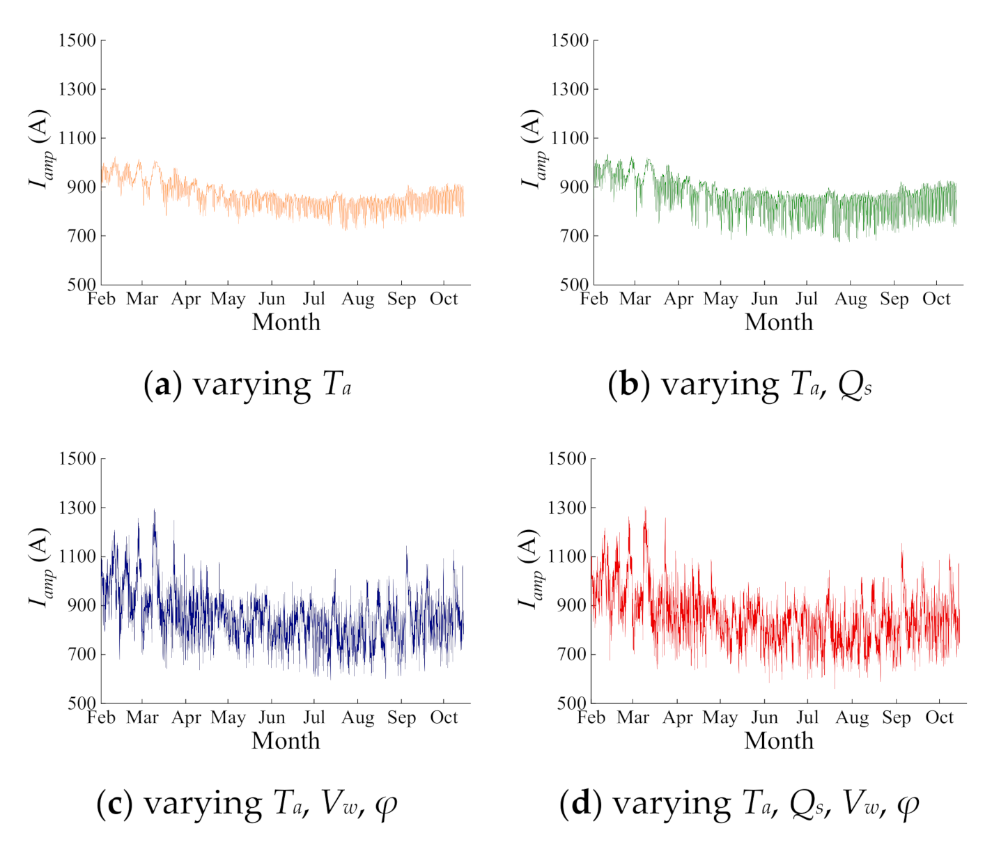
3.1. Collective Influence of Multiple Weather Parameters
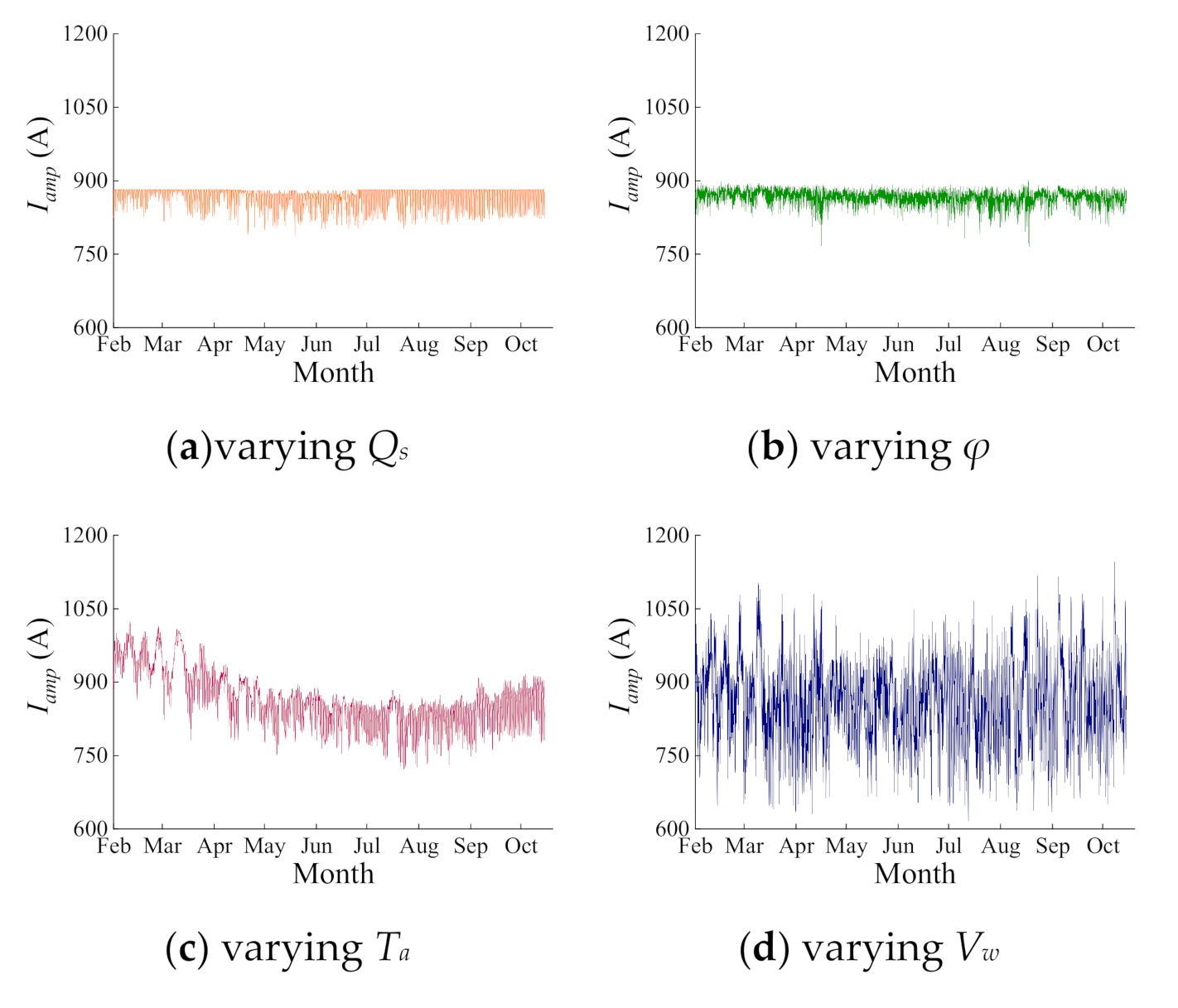
3.2. Relative Importance of Single Weather Parameter
4. EHT Model of Overhead Conductor
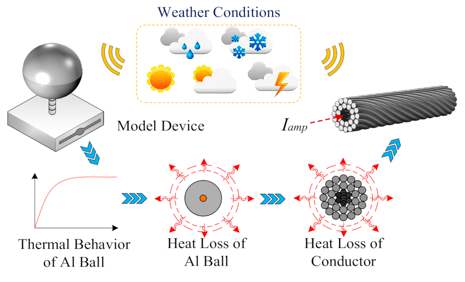
4.1. Model Rationale
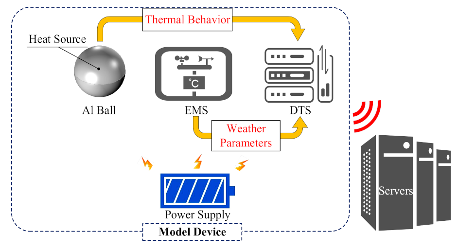
4.2. Model Device
4.3. Calculation for Heat Loss of Al Ball
4.4. Correlation Analysis of Convective Heat Losses between Al Ball and Conductor
4.5. Ampacity Calculation Based on EHT Model
- (1)
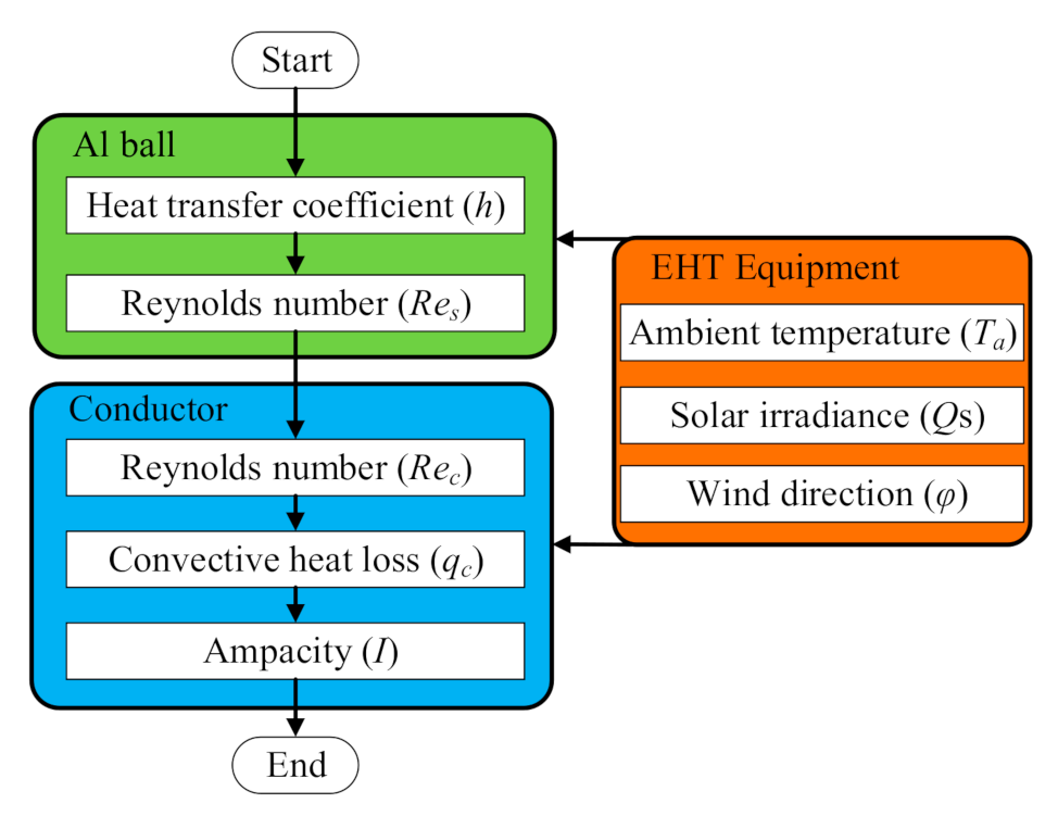
- Calculation of convective heat transfer coefficient of Al ball. The calculation formula for convective heat transfer coefficient of Al ball h is derived according to (11) and (12), as shown in (21). Combined with (21) and the collected weather data collected from the model device, h is calculated.
- (2)
- Calculation of the Reynolds number of the Al ball. After determining the convective heat transfer coefficient of the Al ball, the Reynolds number of the Al ball Res is obtained according to (13)–(14).
- (3)
- Calculation of convective heat loss rate of conductor. Based on the correlation function for the Reynolds numbers of the conductor and Al ball (i.e., (20)), the Reynolds number of the conductor Rec can be calculated. Then, the convective heat loss rate of conductor is also determined by the calculated Rec and (3)–(8).
- (4)
- Calculation of Iamp. Using the ambient temperature, global solar irradiance collected by the model device and the obtained convective heat loss rate of conductor in step (3), Iamp is calculated through (2).
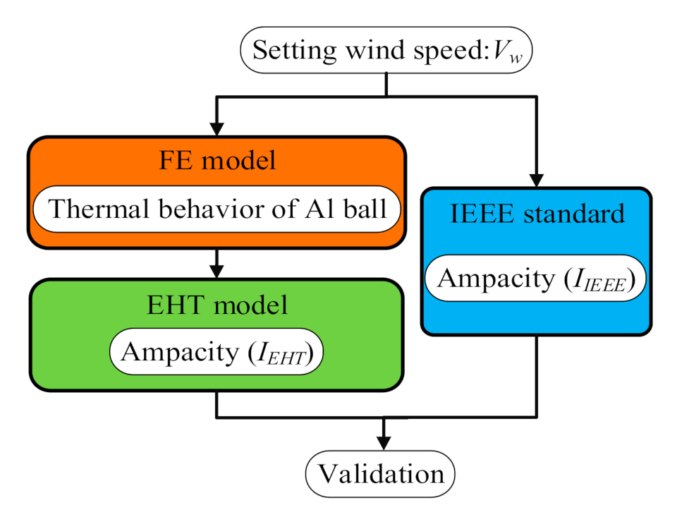
5. Validation of EHT Model Based on FEM
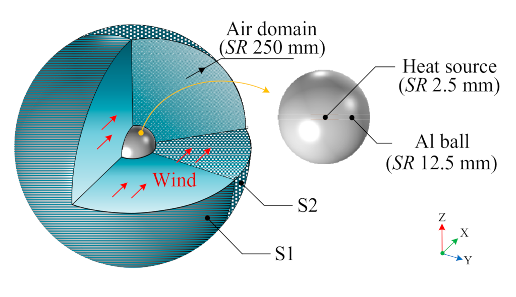
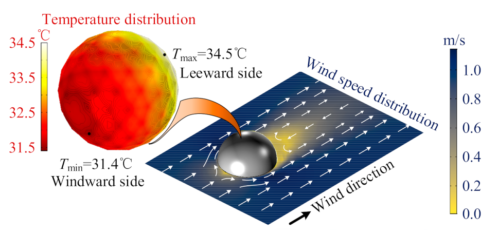
5.1. Setting and Results of FEM
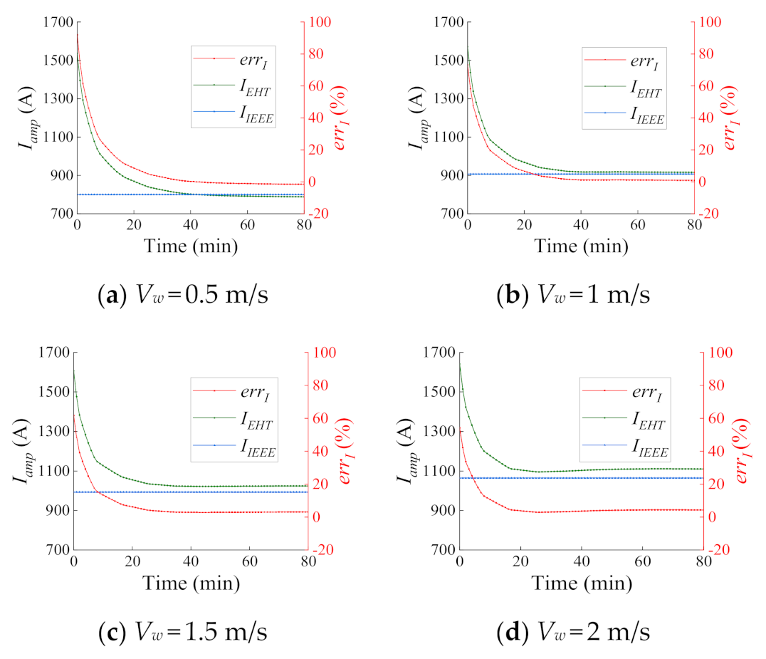
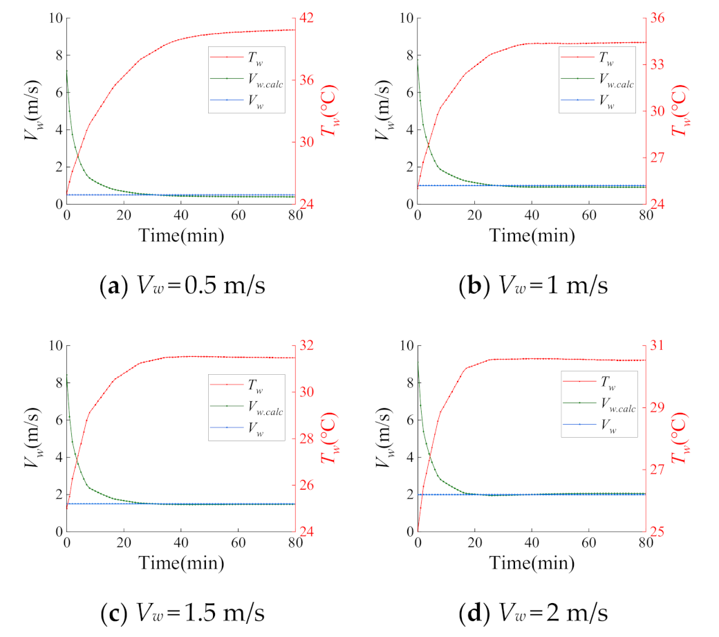
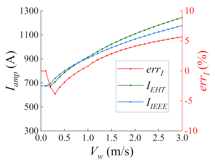
5.2. Validation of EHT Model
6. Conclusions
Author Contributions
Funding
Acknowledgments
Conflicts of Interest
Nomenclature
| Variables | |
| qc | convective heat loss rate of conductor per unit length |
| qr | radiative heat loss rate of conductor per unit length |
| qs | solar heat gain rate of conductor per unit length |
| I | conductor current |
| Tc | conductor temperature |
| R(Tc) | conductor resistance at the temperature of Tc |
| Tcmax | maximum allowable temperature of conductor |
| Iamp | conductor ampacity |
| qcn | qc in natural convection heat transfer |
| qc1 | qc in forced convection heat transfer at low wind speeds |
| qc2 | qc in forced convection heat transfer at high wind speeds |
| ρf | air density |
| D0 | conductor diameter |
| Ta | ambient temperature |
| kf | thermal conductivity of air |
| Kangle | wind direction factor |
| Rec | Reynolds number of conductors |
| φ | angle between wind and axis of conductor |
| Vw | wind speed |
| μf | dynamic viscosity of air at the mean volume reference temperature |
| σ | Steff-Boltzmann constant |
| ε | emissivity of the conductor surface |
| α | solar absorptivity of the conductor surface |
| Qs | global solar irradiance |
| qcs | convective heat loss rate of the aluminum ball |
| qrs | radiative heat loss rate of the aluminum ball |
| qss | solar heat gain rate of the aluminum ball |
| qgs | internal heat source power of the aluminum ball |
| ms | mass of the aluminum ball |
| Cps | specific heat capacity of the aluminum ball |
| Ts | temperature of the aluminum ball |
| t | time |
| h | convective heat transfer coefficient of the aluminum ball |
| l | diameter of the aluminum ball |
| Nu | Nusselt number of the aluminum ball |
| Res | Reynolds number of the aluminum ball |
| Pr | Prandtl number of the aluminum ball |
| Gr | Grashof number of the aluminum ball |
| μw | dynamic viscosity of air at average surface temperature |
| Cp | specific heat capacity of air |
| g | acceleration of gravity |
| Δt | temperature difference between aluminum ball and environment |
| tm | characteristic temperature of the aluminum ball |
| hf | forced convection heat transfer coefficients of the aluminum ball |
| h0 | natural convection heat transfer coefficient of the aluminum ball |
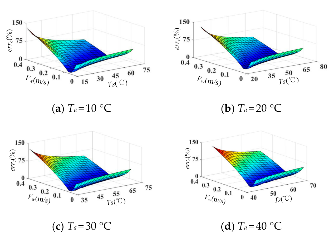
| errc | relative errors between hf and h0 |
| Vwf | calculated specific wind speed |
| IIEEE | conductor ampacity of IEEE standard |
| IEHT | conductor ampacity of EHT model |
| errI | relative errors between IEHT and IIEEE |
| Vw.calc | equivalent wind speed |
| Abbreviations | |
| STR | static thermal rating |
| DTR | dynamic thermal rating |
| EHT | equivalent heat transfer |
| FEM | finite element method |
| Al | aluminum |
| EMS | environmental monitoring system |
| DTS | data transmission system |
References
- Mbuli, N.; Xezile, R.; Motsoeneng, L.; Ntuli, M.; Pretorius, J. A literature review on capacity uprate of transmission lines: 2008 to 2018. Electr. Power Syst. Res. 2019, 170, 215–221. [Google Scholar] [CrossRef]
- Song, F.; Wang, Y.; Yan, H.; Zhou, X.; Niu, Z. Increasing the Utilization of Transmission Lines Capacity by Quasi-Dynamic Thermal Ratings. Energies 2019, 12, 792. [Google Scholar] [CrossRef] [Green Version]
- Coletta, G.; Vaccaro, A.; Villacci, D. A review of the enabling methodologies for PMUs-based dynamic thermal rating of power transmission lines. Electr. Power Syst. Res. 2017, 152, 257–270. [Google Scholar] [CrossRef]
- Lai, Q.; Chen, J.; Hu, L.; Cao, J.; Xie, Y.; Guo, D.; Liu, G.; Wang, P.; Zhu, N. Investigation of tail pipe breakdown incident for 110 kV cable termination and proposal of fault prevention. Eng. Fail. Anal. 2020, 108, 104353. [Google Scholar] [CrossRef]
- Uski, S. Estimation method for dynamic line rating potential and economic benefits. Int. J. Electr. Power Energy Syst. 2015, 65, 76–82. [Google Scholar] [CrossRef]
- Liu, G.; Xu, Z.; Ma, H.; Hao, Y.; Wang, P.; Wu, W.; Xie, Y.; Guo, D. An improved analytical thermal rating method for cables installed in short-conduits. Int. J. Electr. Power Energy Syst. 2020, 123, 106223. [Google Scholar] [CrossRef]
- Reddy, B.; Mitra, G. Investigations on High Temperature Low Sag (HTLS) Conductors. IEEE Trans. Power Deliv. 2020, 35, 1716–1724. [Google Scholar]
- Wan, H.; McCalley, J.; Vittal, V. Increasing thermal rating by risk analysis. IEEE Trans. Power Syst. 1999, 14, 815–821. [Google Scholar] [CrossRef]
- Michiorri, A.; Nguyen, H.; Alessandrini, S.; Bremnes, J.B.; Dierer, S.; Ferrero, E.; Nygaard, B.; Pinson, P.; Thomaidis, N.; Uski, S. Forecasting for dynamic line rating. Renew. Sustain. Energy Rev. 2015, 52, 1713–1730. [Google Scholar] [CrossRef] [Green Version]
- Teh, J.; Ooi, C.; Cheng, Y.; Zainuri, M.; Lai, C. Composite Reliability Evaluation of Load Demand Side Management and Dynamic Thermal Rating Systems. Energies 2018, 11, 466. [Google Scholar] [CrossRef] [Green Version]
- Davis, M.W. A new thermal rating approach: The real time thermal Rating System for strategic overhead conductor transmission lines. I. General description and justification of the Real Thermal Rating System. IEEE Trans. Power Appar. Syst. 1977, 96, 803–809. [Google Scholar] [CrossRef]
- Teh, J.; Lai, C.; Muhamad, N.; Ooi, C.; Cheng, Y.; Zainuri, M.; Ishak, M. Prospects of Using the Dynamic Thermal Rating System for Reliable Electrical Networks: A Review. IEEE Access 2018, 6, 26765–26778. [Google Scholar] [CrossRef]
- Dupin, R.; Kariniotakis, G.; Michiorri, A. Overhead lines Dynamic Line rating based on probabilistic day-ahead forecasting and risk assessment. Int. J. Electr. Power Energy Syst. 2019, 110, 565–578. [Google Scholar] [CrossRef]
- Douglass, D.A.; Edris, A.A. Real-time monitoring and dynamic thermal rating of power transmission circuits. IEEE Trans. Power Deliv. 1996, 11, 1407–1418. [Google Scholar] [CrossRef]
- Jiang, J.; Liang, Y.; Chen, C.; Zheng, X.; Chuang, C.; Wang, C. On Dispatching Line Ampacities of Power Grids Using Weather-Based Conductor Temperature Forecasts. IEEE Trans. Smart Grid 2018, 9, 406–415. [Google Scholar] [CrossRef]
- Jiang, J.; Wan, J.; Zheng, X.; Chen, C.; Lee, C.; Su, L.; Huang, W. A Novel Weather Information-Based Optimization Algorithm for Thermal Sensor Placement in Smart Grid. IEEE Trans. Smart Grid 2018, 9, 911–922. [Google Scholar] [CrossRef]
- Michiorri, A.; Taylor, P.C.; Jupe, S.C.E.; Berry, C.J. Investigation into the influence of environmental conditions on power system ratings. Proc. Inst. Mech. Eng. Part A J. Power Energy 2009, 223, 743–757. [Google Scholar] [CrossRef]
- CIGRE Working Group B2. Guide for Thermal Rating Calculations of Overhead Lines; Technical Brochure 601; CIGRE: Paris, France, 2014. [Google Scholar]
- Foss, S.D.; Maraio, R.A. Dynamic line rating in the operating environment. IEEE Trans. Power Deliv. 1990, 5, 1095–1105. [Google Scholar] [CrossRef]
- Bose, A. Smart Transmission Grid Applications and Their Supporting Infrastructure. IEEE Trans. Smart Grid 2010, 1, 11–19. [Google Scholar] [CrossRef]
- Zainuddin, N.; Abd Rahman, M.; Ab Kadir, M.; Ali, N.; Ali, Z.; Osman, M.; Mansor, M.; Ariffin, A.; Abd Rahman, M.; Nor, S.; et al. Review of Thermal Stress and Condition Monitoring Technologies for Overhead Transmission Lines: Issues and Challenges. IEEE Access 2020, 8, 120053–120081. [Google Scholar] [CrossRef]
- Monseu, M. Determination of thermal line ratings from a probabilistic approach. In Proceedings of the Third International Conference on Probabilistic Methods Applied to Electric Power Systems (Conf. Proc. No.338), London, UK, 3–5 July 1991; pp. 180–184. [Google Scholar]
- Zhao, Y.; Han, Z.; Xie, Y.; Fan, X.; Nie, Y.; Wang, P.; Liu, G.; Hao, Y.; Huang, J.; Zhu, W. Correlation Between Thermal Parameters and Morphology of Cross-Linked Polyethylene. IEEE Access 2020, 8, 19726–19736. [Google Scholar] [CrossRef]
- Xie, Y.; Zhao, Y.; Bao, S.; Wang, P.; Huang, J.; Liu, G.; Hao, Y.; Li, L. Rejuvenation of Retired Power Cables by Heat Treatment: Experimental Simulation in Lab. IEEE Access 2020, 8, 5635–5643. [Google Scholar] [CrossRef]
- Ghafourian, M.; Bridges, G.E.; Nezhad, A.Z.; Thomson, D.J. Wireless overhead line temperature sensor based on RF cavity resonance. Smart Mater. Struct. 2013, 22, 075010. [Google Scholar] [CrossRef]
- Li, Q.; Zhou, Z.; Zhou, W.; Wei, J.; Wang, K.; Liu, G.; Deng, H.; Wang, P.; Shu, J. A case study on an explosion accident of a 110 kV porcelain housed MOA. Eng. Fail. Anal. 2020, 115, 104665. [Google Scholar] [CrossRef]
- Lecuna, R.; Castro, P.; Manana, M.; Laso, A.; Domingo, R.; Arroyo, A.; Martinez, R. Non-contact temperature measurement method for dynamic rating of overhead power lines. Electr. Power Syst. Res. 2020, 185, 106392. [Google Scholar] [CrossRef]
- Olsen, R.; Edwards, K. A new method for real-time monitoring of high-voltage transmission-line conductor sag. IEEE Trans. Power Deliv. 2002, 17, 1142–1152. [Google Scholar] [CrossRef]
- Seppa, T.O. Accurate ampacity determination: Temperature-sag model for operational real time ratings. IEEE Trans. Power Deliv. 1995, 10, 1460–1470. [Google Scholar] [CrossRef]
- Mahin, A.; Hossain, M.; Islam, S.; Munasinghe, K.; Jamalipour, A. Millimeter Wave Based Real-Time Sag Measurement and Monitoring System of Overhead Transmission Lines in a Smart Grid. IEEE Access 2020, 8, 100754–100767. [Google Scholar] [CrossRef]
- Polevoy, A. Impact of Data Errors on Sag Calculation Accuracy for Overhead Transmission Line. IEEE Trans. Power Deliv. 2014, 29, 2040–2045. [Google Scholar] [CrossRef]
- IEEE. IEEE Std 738-2012: IEEE Standard for Calculating the Current-Temperature Relationship of Bare Overhead Conductors; IEEE Standard Association: Washington, DC, USA, 2013. [Google Scholar]
- Morgan, V.T. Rating of bare overhead conductors for continuous currents. Proc. Inst. Electr. Eng. 2010, 114, 1473–1482. [Google Scholar] [CrossRef]
- CIGRE Working Group 22.12. The Thermal Behaviour of Overhead Conductors Section 1 and 2: Mathematical Model for Evaluation of Conductor Temperature in the Steady State and the Application Thereof. Electra 1992, 4, 107–125. [Google Scholar]
- Whitaker, S. Forced convection heat transfer correlations for flow in pipes, past flat plates, single cylinders, single spheres, and for flow in packed beds and tube bundles. AICHE J. 1972, 18, 361–371. [Google Scholar] [CrossRef]
- Taylor, C.S.; House, H.E. Emissivity and Its Effect on the Current-Carrying Capacity of Stranded Aluminum Conductors. Trans. Am. Inst. Electr. Eng. Part 3 1956, 75, 970–976. [Google Scholar]
- Rigdon, W.S.; House, H.E.; Grosh, R.J.; Cottingham, W.B. Emissivity of Weathered Conductors after Service in Rural and Industrial Environments. Trans. Am. Inst. Electr. Eng. Part 3 1962, 81, 891–896. [Google Scholar] [CrossRef]
- Daoush, W.; Swidan, A.; El-Aziz, G.A.; Abdelhalim, M. Fabrication, Microstructure, Thermal and Electrical Properties of Copper Heat Sink Composites. Mater. Sci. Appl. 2016, 7, 542–561. [Google Scholar] [CrossRef] [Green Version]
- Weltner, K. Measurement of specific heat capacity of air. Am. J. Phys. 1993, 61, 661–662. [Google Scholar] [CrossRef]
- Comsol Multiphysics. Heat Transfer Module User’s Guide; Comsol AB Group: Stockholm, Sweden, 2006. [Google Scholar]
- Zhang, T.; Zheng, W.; Xie, Y.; Yuan, J.; Xu, T.; Wang, P.; Liu, G.; Guo, D.; Zhang, G.; Liang, Y. A case study of rupture in 110 kV overhead conductor repaired by full-tension splice. Eng. Fail. Anal. 2020, 108, 104349. [Google Scholar] [CrossRef]
- Velusamy, K.; Sundararajan, T.; Seetharamu, K. Interaction effects between surface radiation and turbulent natural convection in square and rectangular enclosures. J. Heat Transf. Trans. ASME 2001, 123, 1062–1070. [Google Scholar] [CrossRef]

| Feature | Unit | Value |
|---|---|---|
| Rated voltage | kV | 110 |
| Span | m | 300 |
| External diameter | mm | 21.6 |
| Total section | mm2 | 276 |
| Internal layer section (steel) | mm2 | 31.7 |
| External layer section (aluminum) | mm2 | 244 |
| Unitary mass | kg/km | 921.5 |
| Resistance | Ω/km | 0.1181 |
| Statistics | Ta | Ta, Qs | Ta, Vw, φ | Ta, Qs, Vw, φ |
|---|---|---|---|---|
| Min (°C) | 722 | 675 | 596 | 560 |
| Max (°C) | 1024 | 1036 | 1296 | 1305 |
| Range (°C) | 302 | 361 | 700 | 745 |
| Mean (°C) | 866 | 865 | 855 | 855 |
| Standard deviation (°C) | 56 | 69 | 108 | 112 |
| Statistics | Qs | φ | Ta | Vw |
|---|---|---|---|---|
| Min (°C) | 788 | 766 | 722 | 617 |
| Max (°C) | 882 | 902 | 1024 | 1146 |
| Range (°C) | 94 | 136 | 302 | 529 |
| Mean (°C) | 868 | 866 | 866 | 858 |
| Standard deviation (°C) | 19 | 14 | 56 | 85 |
© 2020 by the authors. Licensee MDPI, Basel, Switzerland. This article is an open access article distributed under the terms and conditions of the Creative Commons Attribution (CC BY) license (http://creativecommons.org/licenses/by/4.0/).
Share and Cite
Liu, Z.; Deng, H.; Peng, R.; Peng, X.; Wang, R.; Zheng, W.; Wang, P.; Guo, D.; Liu, G. An Equivalent Heat Transfer Model Instead of Wind Speed Measuring for Dynamic Thermal Rating of Transmission Lines. Energies 2020, 13, 4679. https://doi.org/10.3390/en13184679
Liu Z, Deng H, Peng R, Peng X, Wang R, Zheng W, Wang P, Guo D, Liu G. An Equivalent Heat Transfer Model Instead of Wind Speed Measuring for Dynamic Thermal Rating of Transmission Lines. Energies. 2020; 13(18):4679. https://doi.org/10.3390/en13184679
Chicago/Turabian StyleLiu, Zhao, Honglei Deng, Ruidong Peng, Xiangyang Peng, Rui Wang, Wencheng Zheng, Pengyu Wang, Deming Guo, and Gang Liu. 2020. "An Equivalent Heat Transfer Model Instead of Wind Speed Measuring for Dynamic Thermal Rating of Transmission Lines" Energies 13, no. 18: 4679. https://doi.org/10.3390/en13184679
APA StyleLiu, Z., Deng, H., Peng, R., Peng, X., Wang, R., Zheng, W., Wang, P., Guo, D., & Liu, G. (2020). An Equivalent Heat Transfer Model Instead of Wind Speed Measuring for Dynamic Thermal Rating of Transmission Lines. Energies, 13(18), 4679. https://doi.org/10.3390/en13184679