Article

A Forecasting-Based Control Algorithm for Improving Energy Managment in High Concentrator Photovoltaic Power Plant Integrated with Energy Storage Systems

1
Department of Electric and Electronic Engineering, University of Cagliari, via Marengo 2, 09123 Cagliari, Italy
2
CRS4, Center for Advanced Studies, Research and Development in Sardinia, loc. Piscina Manna ed. 1, 09050 Pula (CA), Italy
*
Author to whom correspondence should be addressed.
Energies 2020, 13(18), 4697; https://doi.org/10.3390/en13184697
Submission received: 7 August 2020 / Revised: 3 September 2020 / Accepted: 7 September 2020 / Published: 9 September 2020
(This article belongs to the Special Issue Advances in Concentrator Photovoltaics and Solar Cells)

Abstract

:
The High Concentrator Photovoltaic (HCPV) technology, due to its high efficiency, is considered one of the most promising solutions for the exploitation of sun-irradiation-based Renewable Energy Sources (RES). Nevertheless, the HCPV production is strictly connected to the Direct Normal Irradiation (DNI) making this photovoltaic technology more sensible to cloudiness than traditional ones. In order to mitigate the power intermittence and improve production programmability, the integration between Energy Storage Systems (ESSs) and HCPV, resorting to forecasting algorithms, has been investigated. Specifically, a local weather forecasting algorithm has been used for estimating the daily time evolution of DNI, air Temperature (T), Wind Speed (WS), and Air Mass (AM). These data are subsequently processed by means of an accurate HCPV model for the estimation of one day-ahead daily power production profile. The processing of HCPV forecasted generation by means of a properly tuned filter-based algorithm allows one day-ahead the definition of power profiles of ESS and power plant respectively, considering also the ESS constraints and the characteristic of the implemented real-time control algorithm. The effectiveness of the proposed forecasting model and control algorithm is verified through a simulation study referring to the solar power plant constituted by HCPV and ESS installed in Ottana, Italy. The results highlight that the application of the proposed approach lessens the power fluctuation effect caused by HCPV generation preserving the batteries at the same time. The feasibility and advantages of the proposed approach are finally presented.

1. Introduction

Nowadays, photovoltaic can be considered a mature technology and it will certainly have in the next future a fundamental role in electricity generation from Renewable Energy Sources (RES). In particular, the High Concentrator Photovoltaic System (HCPV) stands out among the available photovoltaic technologies thanks to the high efficiencies it is characterized by. Compared to the silicon-based monocrystalline cells, the average efficiency of HCPV cell is two times higher, reaching values equal to 41% for commercial cells [1], up to 44% in laboratories [2,3]. Such high values are obtainable thanks to the multi-junction technologies that consist of using multiple layers of different materials each of which reacts to different sunlight wavelengths. This kind of cell achieves its best performance for a specific level of irradiation. For this purpose, an optical concentrator that collects the solar radiation focusing it from 10 to more than 2000 times is installed in HCPV modules [4]. This allows for reducing the photovoltaic active area, limiting significantly the high-performance semiconductor materials required for the same rating power. The main drawback of this technology is related to its Direct Normal Irradiation (DNI) dependence. In fact, cloudiness, tracking errors, and dust sedimentation on the modules strongly affect the collection of DNI on photovoltaic active area and, thus, the HCPV production. While the latter two phenomena can be mitigated or avoided by improving the tracking performances and periodically cleaning modules respectively, the effects on the HCPV associated with cloudiness require the introduction of specific solutions. In fact, the cloudiness effects, amplified by optical concentration, introduces sudden and significant DNI fluctuations, affecting the power quality of electricity delivered to the grid. A general approach proposed in the technical literature to overcome this issue is the integration of photovoltaic (PV) power plants with Energy Storage Systems (ESSs) managed for improving power quality and production programmability. Several works concerning the integration of traditional PV with ESS have been presented, some aimed at smoothing the time evolution of power profile delivered to the grid [5], others oriented to reproduce a flat band power profile resorting to high-capacity storage [6]. In this context, the use of weather forecasting algorithms improve the the performance of PV-ESS power plants in terms of programmability and power quality [7].
In fact, the combination of energy management strategies with accurate wheater forecast algorithms could guarantee greater predictability of photovoltaic production improving consequently the integration of PV into the power system. However, the greater susceptibility of HCPV to the environmental conditions and specifically to DNI requires that the forecasting algorithms be properly integrated with real-time control of the power production delivered to the grid.
In this context, the development of a control algorithm suitable for an HCPV power plant supported by ESS has been investigated. The aim of the present paper consists of combining a one-day ahead forecast production algorithm with real-time PV smoothing controls in order to improve the performance in terms of power quality and production programmability. For this purpose, three different real-time PV smoothing control algorithms proposed in the technical literature (the Ramp-Control (RC), the Moving Average (MA), and the Step-Rate (SR) smoothing algorithms [5]) have been considered for HCPV and compared with the proposed configuration that integrates them with one day ahead forecasting and a Filter Based Management (FBM) algorithm. The performance comparison highlights which combination improves better battery utilization and the smoothing effect in the HCPV+ESS power plant.
The comparison has been developed through a simulation study performed in a Matlab-Simulink environment, by considering as a case of study the integrated HCPV-ESS power plant installed in Ottana, Italy, for which the data set and the measurements for training the forecasting algorithm, and for tuning the HCPV modeling, are available—thus, for comparing the power profile improvement, referring to real data of production.
The paper is structured as follows: the proposed configuration of energy managment system (EMS) for HCPV and ESS power plant is described in Section 2 and the case of study is reported in Section 3. In the following sections, the single block of the proposed EMS is described in detail referring to case of study. Specifically, power production forecasting methods are presented in Section 4, whereas the FBM algorithm is presented in Section 5, the smoothing algorithms, and their coupling with FBM in Section 6. Results are presented and discussed in Section 7 and Section 8, respectively.

2. Proposed Configuration of HCPV and the ESS Energy Managment Algorithm

The proposed control algorithm for the energy management of an HCPV power plant integrated with an ESS system is schematically reported in Figure 1. The energy management system is characterized by the presence of two main blocks; the first one is devoted to estimate one-day ahead the daily power profiles of HCPV and to define the proper daily power profiles of ESS according to the system constraints; the second one is the real-time control. In particular, the one-day ahead estimation is based on the use of a weather forecasting algorithm that provides the main information for HCPV daily power profile estimation. Specifically, the weather forecasting provides the DNI, environment Temperature (T), Wind Speed (WS), and Air Mass (AM) using different approaches, such as Numerical Weather Prediction (NWP), Cloud Motion Vector (CMV), and time series analysis. These data support linear models to determine the forecasted power production of HCPV. The linear models considered are the American Society for Testing and Materials (ASTM) model, a modified ASTM that considers also the AM, the Fernández, a modified Fernández that considers also the WS, and a novel model realized by hybridizing the two modified models [8,9]. Subsequently, after the forecasting of the HCPV power profile, a novel FBM algorithm for peak shaving is executed. The chosen FBM is a two-threshold-FBM [10] and it has been modified in order to take care of drops in the power profiles, to fix the State of Charge (SoC) at the end of the day at a specific range of values and by considering a zero-phase low-pass Finite Impulse Response (FIR) filter. The synthesized one-day ahead power profile of ESS is then used as a reference power set-point. During the application of the one-day ahead power set-points, the real-time control, constituted by one of the smoothing control algorithm chosen as RC, MA, and the SR, is implemented in order to compensate the forecasting error by means of proper feedback on the ESS power set point. The proposed control algorithm in terms of weather and HCPV power forecast has been tuned referring to the solar power plant installed in Ottana, Italy. The detail of the algorithm implemented and the simulation results are extensively reported in the following sections.

3. The Case of Study

The Ottana solar facility is sited in Sardinia, Italy. Its main aim is to evaluate the reliability, potentiality, and effectiveness of Concentrating Solar Power (CSP) technologies for distributed generation applications characterized by power sizes lower than 5 MW. The Ottana concentrating solar power plant integrates a small scale CSP and a concentrating photovoltaic (CPV) system with electrochemical ESS and Thermal Energy Storage systems (TES) in order to evaluate the performance obtainable by concentrating solar facility in planning one-day ahead power output. In order to be able of managing the power fluctuations, the energy storage systems have been properly designed and controlled considering the support of weather forecasting service.
In particular, the proposed management strategy consists of two control algorithms: the first is addressed to synthesize the “one-day ahead” optimal scheduling, and the second performs a real-time smoothing control. The Ottana solar power plant is located in the center of Sardinia (Italy), and it is characterized by a 630 kWe CSP plant and a 400 kWe HCPV plant. As previously mentioned, the facility has been provided with both a thermal and an electric storage system. The CSP side is made up of a solar field based on Fresnel technology coupled to a power block based on Organic Rankine Cycle (ORC) unit. The ORC technology allows for operating with partial and with different input conditions without decreasing drastically its efficiency. Moreover, ORCs below 5 MWe are characterized by an interesting conversion efficiency, from thermal energy to electric energy.
The CSP field covers a net aperture area of about 8600 m2, and it generates a thermal power of about 5 MW at a reference irradiation condition. A diathermic oil works as heat transfer fluid and is characterized by a working temperature of 165 °C (inlet) and 275 °C (outlet). CSP is also equipped with two tanks for thermal storage, characterized by a capacity of about 15 MWhth, which means about 5 h of full-load operation. The HCPV side is constituted by 36 two-axis solar trackers, characterized by an overall power of about 400 kWp. A four-quadrant solar sensor and an onboard meteorological station, for measuring the DNI and the wind speed, have been installed on each solar tracker. The system combines astronomical ephemerides and solar tracker information in order to follow continuously the sun position.
The ESS consists of a Sodium-Nickel (NaNiCl) battery characterized by a capacity of 430 kWh and a maximum power of 300 kW. The ESS has been sized considering the expected power fluctuations occurring on HCPV systems as well as their dynamics, which results in being much greater if compared to those of the CSP plant. In particular, the system has been designed in order to allow the compensation of forecasting errors and a predictable generation of HCPV characterized by a time interval of 30 s.
The block diagram of the solar facility and the overview are reported in Figure 2 and Figure 3, respectively.

4. HCPV Production Forecasting

The present section regards the forecast procedure. The first subsection presents the weather forecast algorithm, while the second one describes the five linear models adopted to forecast the power production on the basis of the forecast weather parameters.

4.1. Forecasting Method

Solar radiation forecasting can be achieved using different approaches, such as NWP, CMV, and time series analysis, the application and effectiveness of these techniques depend both on the weather-climate characteristics of the site and the lead time of the forecast itself.
DNI forecasting, in particular, is a challenge, given the greater variability with respect to e.g., wind intensity, temperature, or Global Horizonthal Irradiation (GHI), mainly due to fluctuations in cloud cover [11]. The research work is also affected by the low availability of DNI measurements.
In order to provide an operational service for DNI forecasting, for a specific site, it has been chosen in this case to exploit the potential of a non-specific weather forecast service (DarkSky https://darksky.net). The service for the area of interest and the forecast horizon is mainly based on the results of National Oceanic and Atmospheric Administration (NOAA)’s Global Forecast System (GFS) global atmospheric circulation model (https://darksky.net/attribution) does not provide a direct estimate of GHI or DNI, but provides, in addition to air temperature and ground wind speed, an estimate of cloud cover, on an hourly basis and with a forecast horizon of one week. The cloud cover data are used to obtain an estimate of both GHI and DNI irradiance through a modulation of irradiance under Clear Sky conditions.
In particular, by following the approach described in [12], the GHI radiation can be calculated as:
G H I = ( o f f s e t + ( 1 o f f s e t ) ( 1 C C ) ) G H I c s ,
where G H I c s is the GHI in Clear Sky conditions calculated according to [13], and C C is the expected Cloud Cover, null in Clear Sky conditions and unitary for overcast sky. The o f f s e t parameter allows for calibrating the relationship between C C and the ratio between G H I and G H I c s , in [12], which is taken equal to 0.35 . DNI radiation is calculated in a similar way, using the approach described in [14] :
D N I = ( o f f s e t + ( 1 o f f s e t ) ( 1 C C ) ) D N I c s ,
where D N I c s represents the estimate of the Clear Sky direct radiation assessed according to [13]. The o f f s e t parameter in [14] is null.
The Diffuse Horizonthal Irradiation (DHI) finally results:
D H I = G H I D N I c o s ( z ) ,
where z is the zenith angle of the Sun.
Equation (1) was based on cloud cover forecasts obtained from two publicly-available NWP models: the North American Mesoscale Forecast System (NAM) of NOAA and the Regional Deterministic Prediction System (RDPS) of the Canadian Meteorological Center, while global radiation measurements were collected through two pyranometers located in California. Equation (2) was derived from the RDPS cloud cover forecast and direct irradiance data for stations located in the United States. It remains to be verified whether these models can be valid using forecasts from a different weather service and whether they are applicable to a different geographical area.

4.2. HCPV Production Linear Model

The models described in the following subsections belong to the family of models that evaluate HCPV production by means of a linear regression based on specific atmospheric parameters.
The models analyzed are those that best suit their application on the experimental power plant in Ottana. In fact, none of these require invasive procedures as the measurement of the cell temperature or the determination of the I-V characteristic, nor the application of algorithms based on neural networks. Instead, only the measurement of environmental and production parameters is needed, which is already implemented in the power plant and therefore available at no additional costs.
Three of the following models consider the AM as parameter. For its determination, the following equation by Sandia’s laboratory has been used [15]:
A M ( t ) = p p 0 · c o s ( z ) + 0.50572 · ( 96 . 079950 z ) 1.6364 1
where z represents the zenith angle, p the local pressure in bar, and p 0 the reference pressure in bar. The value of the zenith angle ( z ) is determined by the procedure explained in [16]. For each model, the coefficient associated with a specific parameter is expressed as c n .

4.2.1. Model of the Standard ASTM

The ASTM model considers as parameters the DNI, the T, and the WS. The estimated ideal power production is expressed as:
P h c p v = D N I · ( c 1 + D N I · c 2 + T · c 3 + W S · c 4 )
It is worth noting that the influence of the spectral effects is not taken into account and this is significant considering multijunction solar cell modules [8].

4.2.2. Model of E.F. FernáNdez et al.

The model developed by Fernández et al. [9] considers the spectral influence on the power production by using the AM. Thanks to this approximation, there is no need for any spectroradiometer or isotype cell [8]. The following model considers the influence of AM negligible when A M t h r e value is less than 2 [9]. Therefore, the characteristic equations are:
P h c p v = c 1 · D N I + c 2 · T a i r f o r A M A M t h r e P h c p v = c 1 · D N I + c 2 · T a i r + c 3 · A M f o r A M > A M t h r e

4.2.3. Modified Model of the Standard ASTM

In order to consider the AM influence, as explained above, in the equation of the ASTM, a term associated with the AM has been added. Therefore, the AM is characterized by the equation:
P h c p v = D N I · ( c 1 + D N I · c 2 + T a i r · c 3 + W S · c 4 + A M · c 5 )

4.2.4. Modified Model of E.F. FernáNdez et al.

As Fernández explained in [9], the wind influence is negligible for wind speed values lower than 2 m/s. If the wind speed is higher than this value for almost the whole year, a term that considers its effect can be added to the equation of the Fernández model. In this model, A M t h r e is still considered equal to 2. Therefore, the equations related to the Modified-Fernández are as follows:
P h c p v = c 1 · D N I + c 2 · T a i r + c 3 · W S f o r A M A M t h r e P h c p v = c 1 · D N I + c 2 · T a i r + c 3 · W S + c 4 · A M f o r A M > A M t h r e

4.2.5. A Novel Hybrid Model

By the hybridization of the Modified ASTM and the Modified Fernández, a novel model is developed and presented in this paper. The proposed model considers all the previous shown parameters. In particular, both WS and AM are taken into consideration because it is not negligible, in particular considering windy sites (e.g., for the Ottana power plant location). This model is based on the Modified ASTM’s equation but involves the effect of the AM, only if its value is less than A M t h r e , as in the Fernández model and in the Modified Fernández one. The equations associated with the Hybrid model are as follows:
P h c p v = D N I · ( c 1 + D N I · c 2 + T a i r · c 3 + W S · c 4 ) f o r A M A M t h r e P h c p v = D N I · ( c 1 + D N I · c 2 + T a i r · c 3 + W S · c 4 + A M · c 5 ) f o r A M > A M t h r e
In this model, A M t h r e is set equal to 1.45.

5. Battery Energy Management

FBM is an energy management system strategy characterized by the decoupling between high frequency power profile evolution and the low frequency one, as described in [10]. The decoupling action is provided by a properly tuned low-pass filter. In particular, an FIR filter has been chosen. Since the filter acts on forecasting data ( P h c p v ) and not on real-time samples, it has been updated as a zero-phase filter by applying it a second time on the flipped forecasting data array, allowing for avoiding any phase shift. In Figure 4a, an example of filter application is shown.
The FIR output signal ( P H C P V , f i l ) is subsequently processed by the FBM algorithm. The ESS power setpoint returned by the FBM algorithm must observe the following power and energy constraints:
P e s s , m i n P e s s ( t ) P e s s , m a x e e s s , m i n e e s s ( t ) e e s s , m a x
with P e s s , m i n and P e s s , m a x , maximum and minimum battery power values respectively; e e s s , m i n and e e s s , m a x are the minimum and maximum allowable battery energy values, respectively. Since a two threshold FBM algorithm has been chosen [10], the equation for calculating battery power ( P e s s ) is:
P e s s = P H C P V , f i l + r ˜ + P e s s , m i n 0 + P H C P V , f i l + r ˜ 0 P e s s , m a x
in which r ˜ + and r ˜ are the upper and lower threshold, respectively; x y means “saturated between x and y”. In this specific HCPV application, this equation has been modified as follows in order to compensate forecast power drops:
P e s s = P H C P V , f i l + r ˜ + P e s s , m i n 0 + P H C P V , f i l + r ˜ 0 P e s s , m a x + P H C P V , f i l P h c p v P e s s , m i n P e s s , m a x
The equation for battery energy calculation is as follows:
d e e s s d t = 1 η d , e s s P e s s + P e s s 2 + η c , e s s P e s s P e s s 2
with η d , e s s and η d , e s s as battery discharging and charging efficiency, respectively. Both thresholds are initialized to zero. For each iteration, the FBM algorithm calculates power and energy profiles; if one of the constraints in (10) is violated, it opportunely increases the upper threshold or decreases the lower one until no violations are observed. An additional modification of the algorithm proposed in [10] consists of a second application of the same algorithm that is executed subsequently in order to force the battery SoC, at the end of the day, to a chosen range (between 50% and 60% of SoC). This “refine” algorithm has the same logic of the main one, but it analyzes only the last part of the forecast array, from when e b reaches 60% of SoC to the end. In Figure 4b, an example of FBM application is shown, in which it is worth noting the peak shaving effect.

6. Smoothing Algorithms

HCPV energy production is characterized by high frequency fluctuation that can be even faster than traditional photovoltaic (PV) because of the strict dependence to DNI. The transmission system operators (TSO) have a limited response capacity and the greater the percentage of energy production from HCPV/PV, the more these fluctuations can lead to damaging system failures, above all in isolated cases such as islands. Coupling the HCPV/PV plant with an energy storage system with a proper energy management algorithm can lessen this kind of fluctuation. The smoothing algorithms meet these requirements by acting on power ramps inclination. Given any power profile, it is possible to compute the power variation associated with two consecutive values by the following equation [5]:
r h c p v ( t ) = P h c p v ( t ) P h c p v ( t Δ t ) P N o m · Δ t · 100 ;
with P N o m representing the nominal power of the plant.
On the basis of this parameter, different smoothing algorithm can be developed. A generic block scheme of a smoothing algorithm is presented in Figure 5. It is worth noting that P E S S is defined as:
P e s s = P g P h c p v
where P g is the output of the smoothing algorithm and represents the power flowing to the grid. The non-ideal efficiency of the ESS has been considered introducing η p c and η b a t that stand for power converter and battery efficiencies, respectively. To compensate losses associated with the above-mentioned efficiency, an optional feedback should be considered.
In the following subsections, three smoothing algorithms have been described and the maximum allowable ramp value has been named r m a x .

6.1. Ramp Control Algorithm

The ramp control strategy analyzes the output power P g flowing to the grid. After comparing the present P g value to the one of the previous iteration increased and decreased by the maximum allowable ramp, the algorithm saturate P g between these extremes:
P g ( t Δ t ) Δ t · r m a x < P g ( t ) < P g ( t Δ t ) + Δ t · r m a x
In [5], an SoC control has been proposed in order to compensate battery losses and developed by using as feedback action in Figure 5, a proportional gain “K”. Although a value of K between 2 and 8 is recommended, in our case, the system is stable with a value of K equal to 1.2. During the simulation carried out, E r e f has been chosen equal to half of the battery capacity, as suggested in [5].

6.2. Moving Average Algorithm

The second analyzed algorithm smooths the power evolution by computing its mean value on a specific time window T. It could be explained by the following equation:
P g ( t ) = 1 T t T t P h c p v ( t ) d t
Increasing the value of time window T increases the smoothing effect of the moving average algorithm. As in the previous strategy, in [5], a feedback node aimed to compensate the losses has been introduced. In this case, the feedback block contains the integral action reported in the following equations:
P l ( t ) = P e s s P b a t P e ( t ) = 1 T t T t P l ( t ) d t
In Figure 6, the block scheme of this algorithm has been shown.
The feedback action allows for considering the E b a t values at the beginning and at the end of the day equal to each other because it compensates losses and the mean value intrinsically satisfies this requirement. The value of T has been determined by the following equation, reported in [5]:
T = 5400 r m a x

6.3. Step-Rate Control Algorithm

The step-rate control has been presented by Marcos et al. in [5]. This algorithm can be easily explained by the flowchart in Figure 7. As the authors mentioned in [5], this algorithm relies on the high frequency smoothing effect related to interaction near the PV power plant (e.g., 6 km). In this context, a maximum ramp of 2 % in one time step d t is comparable to a maximum ramp of n · 2 % in a time step equal to n · d t . Hence, the algorithm works on a specific time window that lasts n times the sampling time Δ t . It starts by evaluating if the P h c p v is growing or decreasing. In case of growing, the difference between present value and the minimum value within the time window T is compared to n times the maximum allowable Δ P . In case of decreasing, the comparison takes place considering the difference between the present value and the maximum value within T, and the same allowable Δ P . In both cases, the output needed is forced to be equal to the minimum/maximum value added/subtracted by the allowable Δ P .

6.4. Smoothing the FBM Power Output

The following section considers the application of each of the above-explained smoothing algorithm after the FBM, with the aim of running the FBM at the beginning of the day, and one of the smoothing algorithm during the day. In this case, the FBM power constraints are set equal to half of the maximum power (150 kW), while energy constraints are set equal to 30% and 70% of the SoC, instead of 10% and 90% of SoC. Smoothing algorithms have the other half of power available, while, during their application, energy constraints are again set equal to 10% and 90% of SoC. In order to better simulate the real operative conditions, the FBM works on forecasting data modified with two power drops; then, for the smoothing algorithms step, one more power drop and a 4% noise have been added to the forecast array.

7. Results

The presented results are related to the Ottana power plant in Sardinia. The facility consists of a Fresnel-based CSP plant (8400 m2 of net aperture), having oil as Heat Transfer Fluid (HTF), connected to an ORC turbine (gross power of 664 kW e), a direct two-tank TES system (capacity of about 15 MWhth ), a biaxial tracking CPV power plant (429 kW e) and a Sodium-Nickel (NaNiCl) Energy Storage System (ESS) with a capacity of 430 kWh and a maximum power of 300 kW.

7.1. Forecast Results

Equations (1) and (2) for the estimation of irradiance components from the cloud cover have been verified in [12,14] on measuring stations in the US territory and using different NWP tools. The validity of the approach has also been verified for the different geographical areas and for a different weather forecast service. The method has been here applied to the cloud cover forecasts obtained for the coordinates of the Elmas (CA) airport for a reference year, with hourly resolution, and compared the estimates with the historical series of GHI radiation and DNI horizontal plane projection data from the PVGIS service (https://ec.europa.eu/jrc/en/pvgis) [17], both using the European Center for Medium-Range Weather Forecasts (ECMWF) model reanalysis database (ERA5) and the reference database derived through satellite data processing (SARAH). The optimal offset parameter value has been estimated for both equations by optimizing the Root Mean Square Error (RMSE) error.
Figure 8 shows, through scatterplot, the comparison between the estimated value and the value observed for GHI and for the DNI projection for the ERA5 and SARAH datasets. Figure 9 shows the forecast errors with respect to the ERA5 database through histograms and box-plots. A good match may be noticed and also verified by the values of Mean Bias Error (MBE), Mean Absolute Error (MAE), RMSE, and correlation coefficients, reported in Table 1. The table also reports the value of the Skill Score s s of the forecast evaluated with respect to the RMSE error of a reference forecast obtained through the persistence of irradiation with a lag of 24 h, which is a good estimate for a forecast horizon of one day when no tools are available for the meteorological forecast:
s s = 1 R M S E R M S E p e r s
Only the instants for which the zenith angle is less than 90° have been considered. The table shows the results both for the offset parameter value of the [12,14] papers and, for the optimal offset value, it has been estimated in 0.60 for GHI and 0.20 for DNI. The difference in the optimal value of the offset is mainly due to the different meteorological product used for the cloud cover estimation. The error and skill score values are in line with those found both in the works already mentioned, and, in the most recent studies on the subject, see, for example, [11,18] with variations that are related to the meteorological characteristics of the geographical areas considered.
From Figure 8, it can be noticed how a part of the points of the scatter plot appear aligned on the diagonal; these are the moments in which the weather forecast has correctly estimated a null cloud cover, so the value of the irradiation corresponds to the Clear Sky that is well approximated by the Ineichen model adopted. There is also a second marked line where the points are aligned, close to the diagonal. These are points where the estimated cloud cover is very low, but the weather model can not correctly predict Clear Sky conditions or it overestimates the Cloud Cover coefficient. The results in Figure 9 show a skewness in the distribution of prediction errors, in accordance with the results of previous works. In the same figure, the box-plots show how prediction errors clearly depend on the time of day, due to varying available Clear Sky irradiation. The month-specific box-plots highlight a more uncertain forecast in the spring months due to higher cloudiness compared, for example, to the summer months, where the forecast error is, on average, lower despite higher Clear Sky irradiation. The figure also shows how forecast errors for DNI are significantly higher compared to GHI prediction errors. An improvement in forecasting can clearly be accomplished through better upstream weather forecast output, if available, by obtaining more detailed cloud cover estimation, especially for low cloudiness. A second methodology consists in the post processing of these results, which necessarily passes from a measurement of the radiation on site, possibly carried out in real time in order to exploit the feedback information on the differences between forecast and measurement. Further improvements for very short term forecasting can be achieved through the processing of satellite or sky-camera images installed on site, using optical flow techniques. In any case, the skill score values detected already demonstrate in these conditions the benefit of weather forecasting tools for radiation prediction.

7.2. Linear Model Results

The linear regression has been carried out in the Matlab environment. The first step consists of determining the solar position by the algorithm in [16], then calculating the AM value [15] and loading the measured data. In the second step, each linear regression equation has been applied in order to determine its related coefficients. In the third step, each model’s power forecast has been calculated and compared to the real power production.
The model characterized by the lower Normalized Root Mean Square Error (N-RMSE) is the Hybrid Model as shown in Table 2. Linear coefficients adopted are shown in Table 3.

7.3. Smoothing Algorithm Results

In the following simulations, the maximum allowable ramp value has been set equal to 2%. The three presented smoothing algorithms have been tested on two different power profiles representing a sunny day and a cloudy one. In both cases, three power drops have been added, in order to test the algorithm in worst cases, and a 4% noise in order to simulate more realistic conditions. No procedure reported in [5] that regards the battery sizing has been carried out because the storage system has been previously chosen, and it is operative at the present time in the Ottana power plant. As reported in [5], in order to improve the performance of each algorithms, the initial SoC has been set equal to 50% for RC and SR and 10% (the technical minimum value) for MA. The application of Ramp-control, Moving average control, and Step-rate control on a cloudy day has been shown on the left in Figure 10, Figure 11 and Figure 12, respectively, while Figure 10, Figure 11 and Figure 12 on the right show the same models in a sunny day case.
The same control algorithms have been applied after the application of the two thresholds FBM. Table 4 shows the main parameters of the FIR filter chosen.
As in the previous section, the following figures highlight the effect of this procedure on a power profile related to a cloudy day and to a sunny one.
Figure 13, Figure 14 and Figure 15 on the left shows the cloudy day condition and on the right the sunny day one, for Ramp-Control, Moving Average, and Step-Rate, respectively.
With the aim of better understanding the effectiveness of the twelve analyzed cases, three indicators have been chosen. The first one is the mean value of ramps, measured both on cloudy and sunny day, associated with the power profile without any control strategy and with each one of the six studied. Referring to (14), it can be expressed as:
M e a n R a m p = m e a n ( r h c p v ) ;
Table 5 shows the results.
Moreover, another parameter chosen is the number of ramp sign variation (from positive to negative and vice-versa), as an indicator of noise in the grid power profile. It can be determined by the following condition applied to the whole P g array of each control strategy:
i f s i g n [ P g ( i + 1 ) ] s i g n [ P g ( i ) ] R a m p V a r i a t i o n = R a m p V a r i a t i o n + 1 ; e n d
Table 6 shows the results associated with the above-mentioned parameter.
The last indicator considers the difference between the maximum and the minimum value of SoC, in order to determine how much the battery has been used during the day. It can be easily determined for each strategy by the following equation:
S o C R a n g e = m a x ( S o C ) m i n ( S o C ) ;
Results related to this parameter have been shown in Table 7.

8. Discussion

Results shown in Section 7.2 highlight how the Hybrid Model is characterized by the lowest N-RMSE. For this reason, it could be considered more suitable for modeling the Ottana power plant production on the basis of forecast data. The difference between N-RMSE could be explained considering the AM variation range and the strong wind that characterized the power plant site. Regarding the smoothing performances (Section 7.3), in all the cases studied, the application of an FBM before the smoothing algorithm improves the battery utilization. The MA and FBM-MA cases have the lowest number of ramp variations and, in addition, are characterized by a ramp mean value lower than any other methods. In particular, FBM-MA has the lowest ramp mean value with 0.35 % on the cloudy day case and 0.42 % on the sunny day one. Thus, FBM-MA can be chosen as the most suitable for the Ottana power plant because it guarantees the best performance on grid-side and in terms of battery utilization. The synergy between forecasting algorithms and real-time smoothing ones will be investigated further in the future. In particular, different peak-shaving or other kinds of forecast based algorithms could be used. In the future, the possibility to integrate a super capacitor could be also investigated, in order to compensate the high frequency power fluctuation instead of the battery, preserving its life cycle. The chosen linear model and smoothing algorithm will be implemented on an NI-CompactRIO on the Ottana power plant, and they will be tested on site during a long-term campaign.

Author Contributions

Conceptualization, A.S. and A.D.; methodology, A.S.; software, A.S., M.P. and L.M.; validation, A.S. and A.D.; formal analysis, A.S. and L.M.; investigation, A.S.; resources, A.D. and L.M.; data curation, A.S.; writing—original draft preparation, A.S. and L.M.; writing—review and editing, A.D. and M.P.; visualization, A.S.; supervision, A.D.; project administration, A.D.; funding acquisition, A.D. All authors have read and agreed to the published version of the manuscript.

Funding

This research was funded by Regione Autonoma della Sardegna-Accordo di Collaborazione tra Enti Pubblici-Art. 15 della Legge 7 Agosto 1990 No. 241 for the development of the project “Solare Termodinamico per lo sviluppo di una rete per la Gestione Intelligente dell’Energia Elettrica e Termica”—Grant No.: Cup I58i18000350002.

Conflicts of Interest

The authors declare no conflict of interest.

Abbreviations

The following abbreviations are used in this manuscript:
AMAir Mass
ASTMAmerican Society for Testing and Materials
CMVCloud Motion Vector
CSPConcentrating Solar Power
DHIDirect Horizontal Irradiation
DNIDirect Normal Irradiation
ECMWFEuropean Center for Medium-Range Weather Forecasts
ESSEnergy Storage System
FBMFilter-Based Management
FIRFinite Impulse Response
GFSGlobal Forecast System
GHIGlobal Horizontal Irradiation
HCPVConcentrator Photovoltaic
HTFHeat Transfer Fluid
MAMoving Average
MAEMean Absolute Error
MBEMean Bias Error
N-RMSENormalized Root Mean Square Error
NOAANational Oceanic and Atmospheric Administration
NWPNumerical Weather Prediction
NAMNorth American Mesoscale Forecast System
ORCOrganic Rankine Cycle
PVPhotovoltaic
RESRenewable Energy Sources
RCRamp Control
RDPSRegional Deterministic Prediction System
SoCState of Charge
SRStep Rate
TEnvironment Temperature
TESThermal Energy System
TSOTransmission System Operator
WSWind Speed

References

  1. Browne, B.; Lacey, J.; Tibbits, T.; Bacchin, G.; Wu, T.-C.; Liu, J.Q.; Chen, X.; Rees, V.; Tsai, J.; Werthen, J.-G. Triple-junctionquantum-well solar cells in commercial production. In Proceedings of the 9th International Conference on Concentrating Photovoltaic Systems (CPV-9), Miyazaki, Japan, 15–17 April 2013; pp. 3–5. [Google Scholar]
  2. Sasaki, K.; Agui, T.; Nakaido, K.; Takahashi, N.; Onitsuka, R.; Takamoto, T. Development of InGaP/GaAs/InGaAs inverted triple junction concentrator solar cells. In Proceedings of the 9th International Conference on Concentrator Photovoltaic Systems: CPV-9, Miyazaki, Japan, 15–17 April 2013; Volume 1556, pp. 22–25. [Google Scholar]
  3. Pérez-Higueras, P.; Ferrer-Rodríguez, J.P.; Almonacid, F.; Fernández, F. Efficiency and acceptance angle of High Concentrator Photovoltaic modules: Current status and indoor measurements. Renew. Sustain. Energy Rev. 2018, 94, 143–153. [Google Scholar] [CrossRef]
  4. Shanks, K.; Senthilarasu, S.; Mallick, T.K. Optics for concentrating photovoltaics: Trends, limits and opportunities for materials and design. Renew. Sustain. Energy Rev. 2016, 60, 394–407. [Google Scholar] [CrossRef] [Green Version]
  5. Marcos, J.; De la Parra, I.; García, M.; Marroyo, L. Control Strategies to Smooth Short-Term Power Fluctuations in Large Photovoltaic Plants Using Battery Storage Systems. Energies 2014, 7, 6593–6619. [Google Scholar] [CrossRef]
  6. Beltran, H.; Bilbao, E.; Belenguer, E.; Etxeberria-Otadui, I.; Rodriguez, P. Evaluation of Storage Energy Requirements for Constant Production in PV Power Plants. IEEE Trans. Ind. Electron. 2013, 60, 1225–1234. [Google Scholar] [CrossRef]
  7. Perez, R.; Kivalov, S.; Hoff, T.E.; Dise, J.; Chalmers, D. Mitigating short-term PV output intermittency. In Proceedings of the 28th European Photovoltaic Solar Energy Conference and Exhibition (EU PVSEC), Villepinte, France, 30 September–4 October 2013; pp. 3719–3726. [Google Scholar]
  8. Rodrigo, P.; Fernández, E.F.; Almonacid, F.; Pérez-Higueras, P.J. Models for the electrical characterization of high concentration photovoltaic cells and modules: A review. Renew. Sustain. Energy Rev. 2013, 26, 752–760. [Google Scholar] [CrossRef]
  9. Fernández, E.F.; Pérez-Higueras, P.; Garcia Loureiro, A.J.; Vidal, P.G. Outdoor evaluation of concentrator photovoltaic systems modules from different manufacturers: First, results and steps. Renew. Sustain. Energy Rev. 2013, 21, 693–701. [Google Scholar] [CrossRef]
  10. Porru, M.; Serpi, A.; Salimbeni, A.; Damiano, A. An advanced frequency-based energy management of hybrid energy storage systems for microgrids. In Proceedings of the IECON 2017 43rd Annual Conference of the IEEE Industrial Electronics Society, Beijing, China, 29 October–1 November 2017; pp. 7617–7622. [Google Scholar] [CrossRef]
  11. Perdigão, J.; Canhoto, P.; Salgado, R.; Costa, M.J. Assessment of Direct Normal Irradiance Forecasts Based on IFS/ECMWF Data and Observations in the South of Portugal. Forecasting 2020, 2, 130–150. [Google Scholar] [CrossRef]
  12. Larson, D.P.; Nonnenmacher, L.; Coimbra, C.F.M. Day-ahead forecasting of solar power output from photovoltaic plants in the American Southwest. Renew. Energy 2016, 91, 11–20. [Google Scholar] [CrossRef]
  13. Ineichen, P.; Perez, R. A new airmass independent formulation for the Linke turbidity coefficient. Sol. Energy 2002, 73, 151–157. [Google Scholar] [CrossRef] [Green Version]
  14. Nonnenmacher, L.; Kaur, A.; Coimbra, C.F.M. Day-ahead resource forecasting for concentrated solar power integration. Renew. Energy 2016, 86, 866–876. [Google Scholar] [CrossRef]
  15. King, D.L.; Kratochvil, J.A.; Boyson, W.E. Measuring Solar Spectral and Angle-of-Incidence Effects on Photovoltaic Modules and Solar Irradiance Sensors; Sandia National Laboratories: Albuquerque, NM, USA, 1997; p. 3. [Google Scholar]
  16. Reda, I.; Andreas, A. Solar Position Algorithm for Solar Radiation Application; National Renewable Energy Laboratory: Golden, CO, USA, 2008; pp. 3–11. [Google Scholar]
  17. Amillo, A.G.; Huld, T.; Müller, R. A new database of global and direct solar radiation using the eastern meteosat satellite, models and validation. Remote Sens. 2014, 6, 8165–8189. [Google Scholar] [CrossRef] [Green Version]
  18. Lopes, F.M.; Conceição, R.; Silva, H.G.; Fasquelle, T.; Salgado, R.; Canhoto, P.; Collares-Pereira, M. Short-term forecasts of DNI from an integrated forecasting system (ECMWF) for optimized operational strategies of a central receiver system. Energies 2019, 12, 1368. [Google Scholar] [CrossRef] [Green Version]
Figure 1. Block scheme of the procedure presented in this paper.
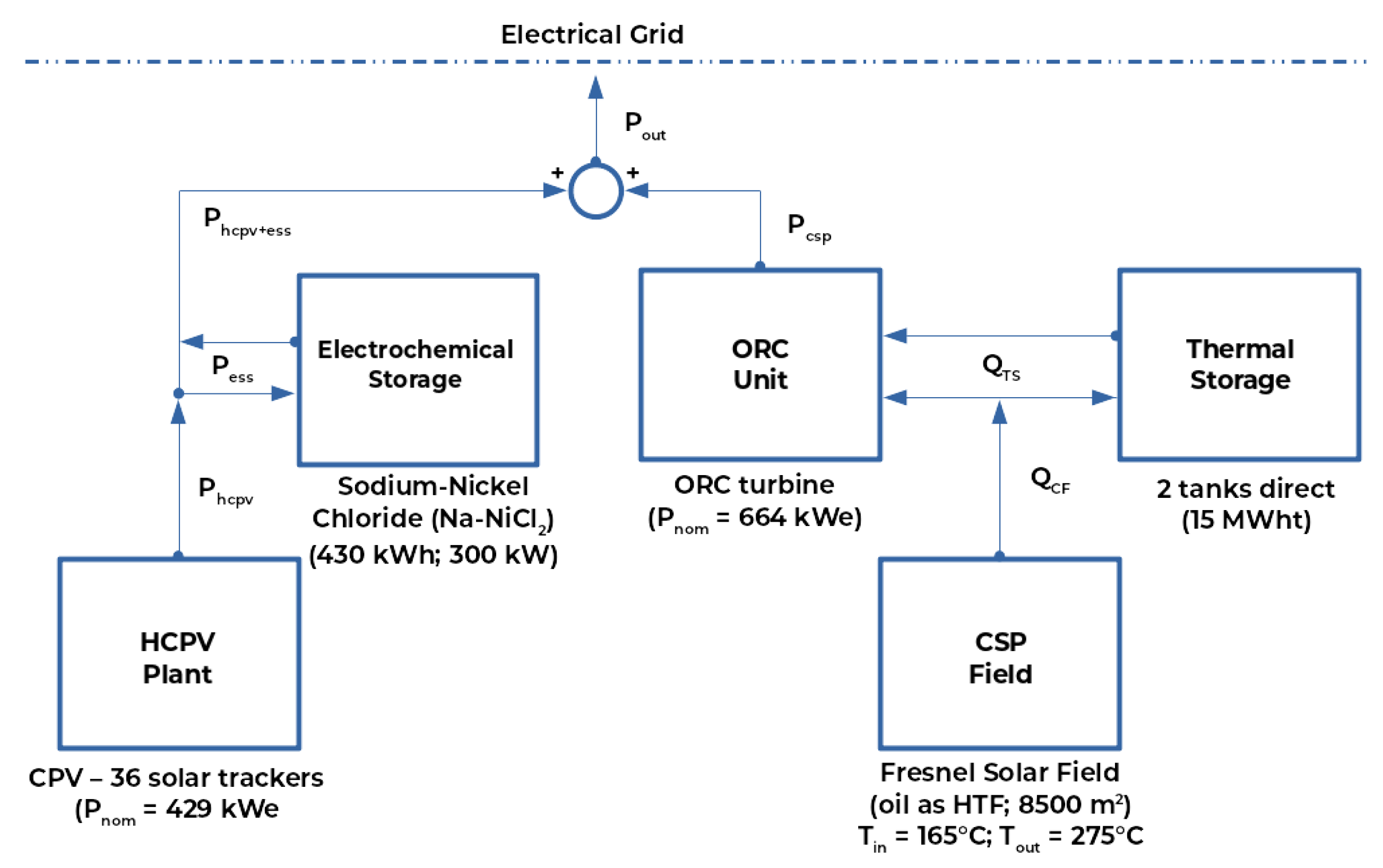
Energies 13 04697 g001
Figure 2. Block diagram of Ottana solar facility used as a case of study.
Energies 13 04697 g002
Figure 3. Overview of the Ottana solar facility.
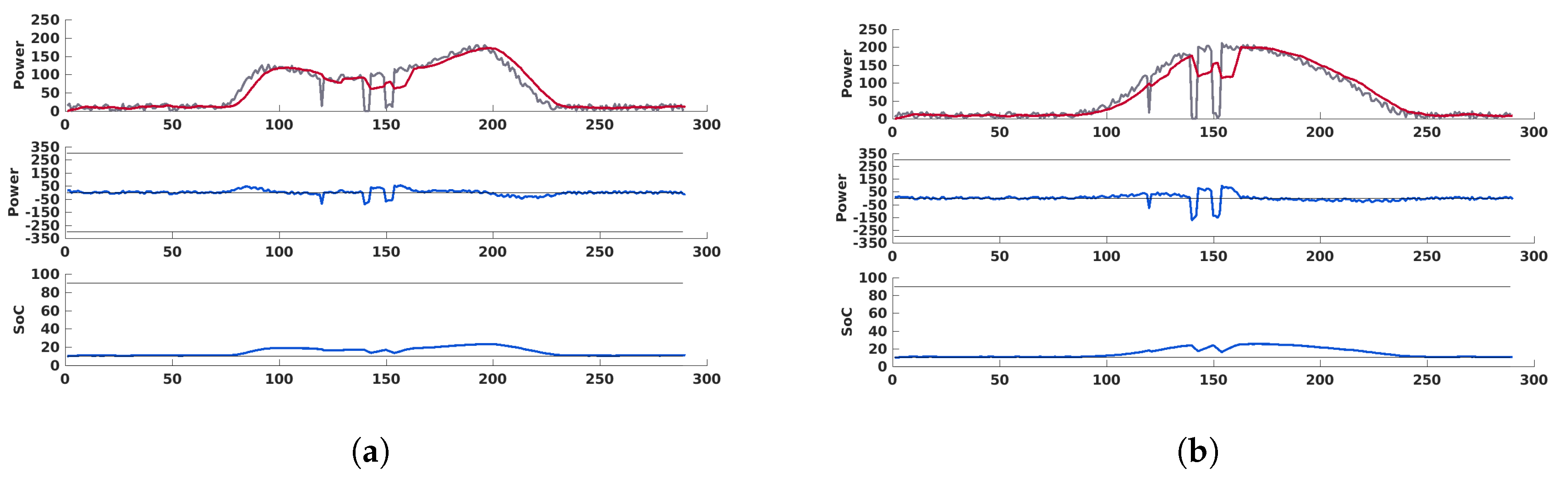
Energies 13 04697 g003
Figure 4. (a) Top: forecast power profile (blue), filtered power profile (red). Bottom: Ideal battery power needed to let flowing to the grid a power equal to the filtered one; (b) Top: Forecast power profile ( P h c p v , grey), power profile after application of FBM ( P g , red); Middle: battery power evolution ( P e s s ); Bottom: battery SoC.
Energies 13 04697 g004
Figure 5. Generic block scheme of a smoothing algorithm. The branch associated with the optional feedback is in red.
Energies 13 04697 g005
Figure 6. Block scheme of the moving average algorithm. The branch associated with the feedback is in red.
Energies 13 04697 g006
Figure 7. Flowchart of the step-rate control algorithm.
Energies 13 04697 g007
Figure 8. Scatterplot of modeled GHI and DNI irradiation on a horizontal surface compared to the measured values from the ERA5 (top) and SARAH (bottom) datasets.
Energies 13 04697 g008
Figure 9. Errors of the modeled GHI and DNI irradiation on a horizontal surface compared to the measured values from the ERA5 dataset. Histograms (first row), box-plot grouped on the hour of the day (second row), and on the month of the year (third row).
Energies 13 04697 g009
Figure 10. Top: Grid power flow with RC ( P g , red) and without RC ( P h c p v , grey). Middle: Battery power evolution ( P e s s , blue) and constraints (grey). Bottom: Battery SoC evolution (blue) and constraints (grey). On a cloudy day case (a), on a sunny day (b).
Energies 13 04697 g010
Figure 11. Top: Grid power flow with MA ( P g , red) and without MA ( P h c p v , grey). Middle: Battery power evolution ( P e s s , blue) and constraints (grey). Bottom: Battery SoC evolution (blue) and constraints (grey). On a cloudy day case (a), on a sunny day (b).
Energies 13 04697 g011
Figure 12. Top: Grid power flow with SR ( P g , red) and without SR ( P h c p v , grey). Middle: Battery power evolution ( P e s s , blue) and constraints (grey). Bottom: Battery SoC evolution (blue) and constraints (grey). On a cloudy day case (a), on a sunny day (b).
Energies 13 04697 g012
Figure 13. Top: Grid power flow with RC ( P g , red) and without RC ( P h c p v , grey). Middle: Battery power evolution ( P e s s , blue) and constraints (grey). Bottom: Battery SoC evolution (blue) and constraints (grey). On a cloudy day case (a), on a sunny day (b).
Energies 13 04697 g013
Figure 14. Top: Grid power flow with FBM-MA ( P g , red) and without FBM-MA ( P h c p v , grey). Middle: Battery power evolution ( P e s s , blue) and constraints (grey). Bottom: Battery SoC evolution (blue) and constraints (grey). On a cloudy day case (a), on a sunny day (b).
Energies 13 04697 g014
Figure 15. Top: Grid power flow with FBM-SR ( P g , red) and without FBM-SR ( P h c p v , grey). Middle: Battery power evolution ( P e s s , blue) and constraints (grey). Bottom: Battery SoC evolution (blue) and constraints (grey). On a cloudy day case (a), on a sunny day (b).
Energies 13 04697 g015
Table 1. Errors for the irradiation model for GHI and DNI, for ERA5 and SARAH datasets, and for the original and optimized offset parameter.
Offset [-]MAE [W/m2]RMSE [W/m2]r [-]ss [-]
GHI (ERA5)0.3553.2885.960.9476.0%
GHI (SARAH)0.3578.06121.370.90316.1%
DNI (ERA5)0.0070.13113.960.87413.2%
DNI (SARAH)0.0095.55149.630.80516.4%
GHI (ERA5)0.6052.0977.170.95721.9%
GHI (SARAH)0.6079.66117.140.91022.7%
DNI (ERA5)0.2066.80102.280.89322.3%
DNI (SARAH)0.2094.31142.490.81617.8%
Table 2. Normalized RMSE associated with each model.
ASTMFernàndezModified ASTMModified FernandezHybrid Model
N-RMSE [%] 6.85121 7.16967 6.81463 7.06794 6.77593
Table 3. Linear coefficient of the production Hybrid model adopted in this paper.
c1c2c3c4c5
A M 1.45 4.46990.0020−0.00690.0276-
A M > 1.45 5.49410.0015−0.01810.0249−0.2040
Table 4. Low-pass FIR filter characteristics.
ParameterValueUnit
TypologyLow-Pass FIR-
Passband Frequency 53.33 μ Hz
Stopband Frequency160 μ Hz
Passband Ripple 0.5 dB
Stopband Attenuation60dB
Sample Rate 3.333 mHz
Design MethodKaiserwin-
Table 5. Ramps’ mean values for each strategy in both cases.
No StrategyRCFBM-RCMAFBM-MASRFBM-SR
Cloudy day1.991.331.270.500.351.681.62
Sunny day2.441.351.370.570.441.801.76
Table 6. Number ramp sign variations for each strategy in both cases.
No StrategyRCFBM-RCMAFBM-MASRFBM-SR
Cloudy day18015316577107181183
Sunny day19017017182115191194
Table 7. Values of Δ S o C for each strategy in both cases.
No StrategyRCFBM-RCMAFBM-MASRFBM-SR
Cloudy day-4.5640.0613.3143.865.1642.00
Sunny day-10.8540.4615.2845.9213.0645.56

