Measurements of Discharge through a Pump-Turbine in Both Flow Directions Using Volumetric Gauging and Pressure-Time Methods

Abstract

This article presents the original procedures for measuring the flow rate using the pressure-time and the volumetric gauging method in the case of performance tests of a reversible hydraulic machine in either turbine or pump modes of operation. Achieving the lowest possible measurement uncertainty was one of the basic conditions during implemented machine tests. It was met using appropriate measuring procedures and high-class measuring equipment. Estimation of the uncertainty for both methods was made on the basis of an analysis consistent with current requirements in this respect. The pressure-time method was supplemented by the computational fluid dynamics (CFD) analysis that allowed reducing the impact of the pipeline complex irregular geometry on the uncertainty of flow measurement. Appropriate modifications of the calculation procedure enabled accurate measurements of flow during the pump mode of operation of the tested machine as well. The volumetric gauging method, thanks to a special procedure used for accurate measurement of the water level in the upper reservoir of the power plant, allowed measuring the discharge through the tested reversible machine with very low uncertainty. The obtained results allowed for a detailed comparison and mutual verification of the methods used to measure the discharge of the tested reversible machine in both modes of its operation. The most possible causes of obtained results are discussed and summarized in the paper. The need for further research was pointed out to explain the differences obtained and their influence on the accuracy of discharge measurement using the pressure-time method in pump operation mode.

1. Introduction

Fluid flow rate measurements are one of the most complex measurements that are carried out in engineering practice. These measurements, due to the need to maintain a very narrow uncertainty band, usually require the use of sophisticated, precise measuring equipment and the use of appropriate rigorous measurement procedures [1,2,3].

Liquid flow rate measurements in closed conduits or open channels of small size, for instance up to 1–2 m of diameter, are usually carried out using standard measuring devices such as measuring orifice plates, nozzles, Venturi tubes, measuring weirs, electromagnetic and ultrasound flow meters, calibrated bends, and others. Such devices are usually installed in properly prepared measuring sections of conduits or channels and provide a relatively easy and fairly accurate method of measuring the flow rate.

The situation is definitely more complicated when the liquid flow rate is to be measured in large-size conduits with a diameter of several meters or more. Measurements of the flow rate in this type of structure, usually used in hydropower, are very difficult and expensive, especially when it is necessary to ensure the lowest possible uncertainty of measurement results.

According to international standards [4,5,6], a few primary methods for flow rate measurement can be used in hydropower plants:

• The velocity-area method—utilizing the distribution of local liquid velocities, measured using propeller current meters (especially in cases of large conduit diameters) or Pitot tubes (for smaller diameters and flow of liquids free of sediments). The volumetric flow rate is determined by integrating the velocity distribution over the entire area of the measuring cross-section.
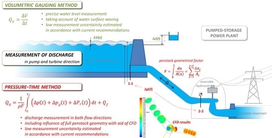
• The pressure-time method (often called the Gibson method [7,8])—consisting of measuring the time course of changes in the pressure difference between two cross-sections of a closed conduit while stopping the liquid stream by means of a shut-off device. The volumetric flow rate of the liquid at the initial conditions, prior to the stoppage of the flow, is determined by appropriate integration of the change in pressure difference measured during the stoppage of the flow.
• The tracer method—consisting of measurements of the passing time, or concentration, of the radioactive or non-radioactive marker (e.g., salt) between two cross-sections of a conduit. The method requires long conduits and suitable conditions for good mixing of the marker.
• The volumetric gauging method—consisting of determining the variation of the water volume stored in the headwater or tailwater reservoir on the basis of the variation of the water level in this reservoir over time.
• The acoustic method—based on vector summation of the sound wave propagation speed and the average liquid flow velocity—it uses a difference in frequencies or passing times of the emitted and received acoustic signal.

It can be concluded that the first four methods on the above list belong to the group of traditional methods, while the acoustic method is relatively new and has been recently the object of numerous research activities oriented on its improvement and validation [9,10]. This method has not yet reached proper acceptance among the specialists. Standard [4] suggests conditional use of this method, i.e., in case of mutual agreement between interested parties. Its basic advantage is that it can be used for continuous flow rate measurement and monitoring. Such a feature is impossible or extremely hard to achieve using other primary methods of measuring absolute flow rate.

The volumetric gauging method and tracer method are those which are less frequently used in hydropower engineering. The first method is characterized by a very limited application, mainly to hydropower plants with artificial reservoirs, especially in pumped-storage plants. The second one requires very long measuring segments of flow conduits and special conditions facilitating the mixing process of the injected markers (e.g., the use of turbulizers).

The velocity-area method and the pressure-time method are primary methods that are the most commonly used for measuring the flow rate in the pipelines of hydraulic turbines [3,11,12,13]. It is also worth noting that the velocity-area method using propeller current meters, very popular in the past, nowadays is being replaced by the pressure-time method in hydropower plants equipped with pipelines longer than 10–20 m. One of the main reasons for this is the much lower cost of preparing and performing flow measurements using the pressure-time method and the use of computer techniques in recent years, which facilitate measurements and give the possibility for getting higher accuracy of results obtained with this method.

For low and very low head power plants, particularly with short intakes of hydraulic turbines, (with no penstocks) the situation is different. Up to now, generally only the velocity-area methods, especially current meter method, are basically available in such kind of plants. Flow rate measurements with this method are still quite expensive and alternatives are being sought. One such alternative is the acoustic scintillation technique, under development [14,15].

Relative (index) methods are also used to measure the flow rate in hydropower plants. For example, the Winter–Kennedy method and the methods utilizing non-standardized pressure difference devices, non-standardized overflows (weirs), some simple variants of the acoustic method or local velocity measurement, which can be used for determining the relative value of the flow rate, or even the physical value, provided that calibration has been done on site by comparing with the results of measurements using the primary method [16,17,18].

As is the case concerning every measurement technique, obtaining the appropriate measurement precision is of the utmost importance. This is absolutely necessary wherever there are low uncertainty requirements, e.g., in the case of performance tests of hydraulic machines. The measurement conditions occurring in the flow systems of these machines require experience and knowledge about the flow phenomena prevailing in these systems, and also force the search for additional, unconventional techniques to ensure sufficiently low measuring uncertainty.

The bases of the analysis presented in the paper are measurement examples of flow rate through a high-head reversible hydraulic machine. Measurements were conducted using the volumetric gauging method and the pressure-time method, recommended (as mentioned earlier) by international standards [4,5,6] as the primary methods for discharge measurements used for performance tests (warranty, acceptance) of hydraulic turbines, pump turbines, and storage pumps. However, there are some restrictions on applicability as in the case of the pressure-time method, but work is continuously ongoing to expand and update these standards (A. Adamkowski, one of the authors of this work is a member of the PTC 18 Committee that is currently developing a revision to the ASME Performance Test Code PTC 18-2011 “Hydraulic Turbines and Pump Turbines”).

The simultaneous application of the pressure-time method and the volumetric gauging method to measure discharge through the tested hydrounit with reversible Francis turbine opened the possibility of their peer verification, which was the main goal of the work.

As part of this task, the suitability of the pressure-time method for measuring flow rate in the pump mode of operation was tested. The use of this method in such conditions is not recommended by standards [4,5,6], therefore the obtained results are of particular importance for the development of this method.

The tests were performed ensuring a low level of measurement uncertainty. It required a number of procedures, some of which are innovative solutions, such as:

• Applying a special procedure for measuring of water level changes in the upper reservoir using the volumetric method.
• Taking into account the complex geometry of measuring section of the pipeline and its impact on flow phenomena using techniques based on computational fluid dynamics (CFD) and applying these results in the pressure-time method.

Moreover, in order to reliably estimate the measurement uncertainty of the applied methods, a procedure that takes into account general requirements concerning uncertainty assessment gathered in [19] has been proposed. This task is an attempt to systematize the problem of estimating measurement errors with the use of the analyzed methods.

Comparison concerning results obtained using chosen flow measurement methods, which is an example quite rarely seen in the literature concerning this subject, provides a unique source of knowledge about the features of the methods and the possibilities of their practical use.

2. Materials and Methods

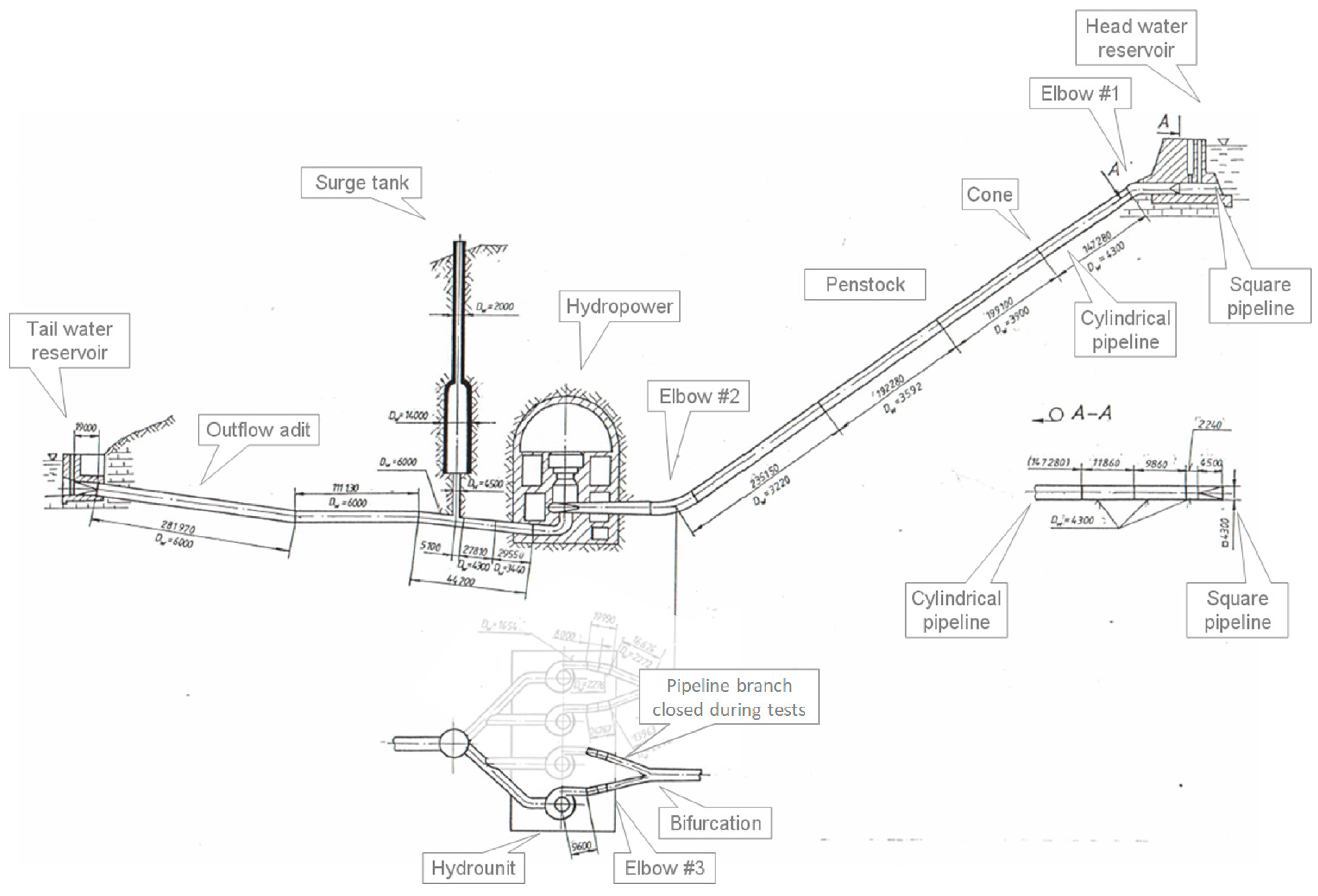
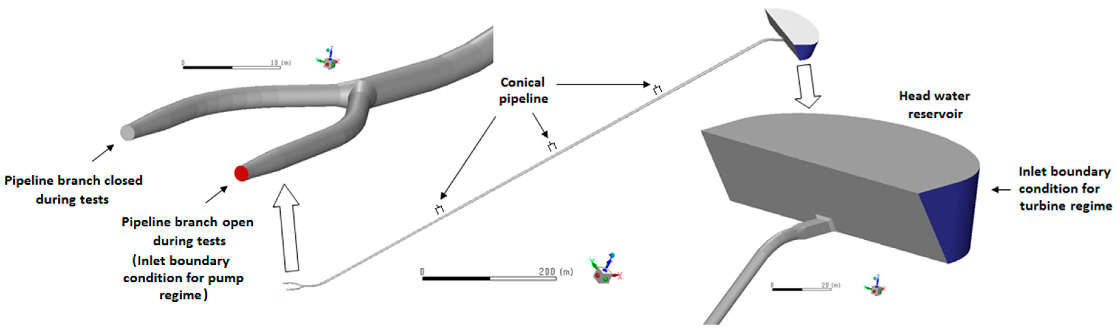
2.1. The Research Object

Both discussed methods for discharge measurement—pressure-time and volumetric gauging method—were used for performance tests of a reversible hydrounit in a Polish pumped-storage power plant (PSPP). The considered plant is equipped with four similar reversible hydraulic machines (pump-turbines) working under the head of approximately 440 m and generating/consuming power over 120 MW.

The artificial head water reservoir is connected to pump-turbines using two underground penstocks, branching close to the inlets of the pump-turbines, prior to the shut-off ball-valves. The pump-turbines are connected via the tailrace tunnel with the surge tank to the tail water tank. A schematic diagram of the PSPP flow system with its main dimensions is shown in Figure 1.

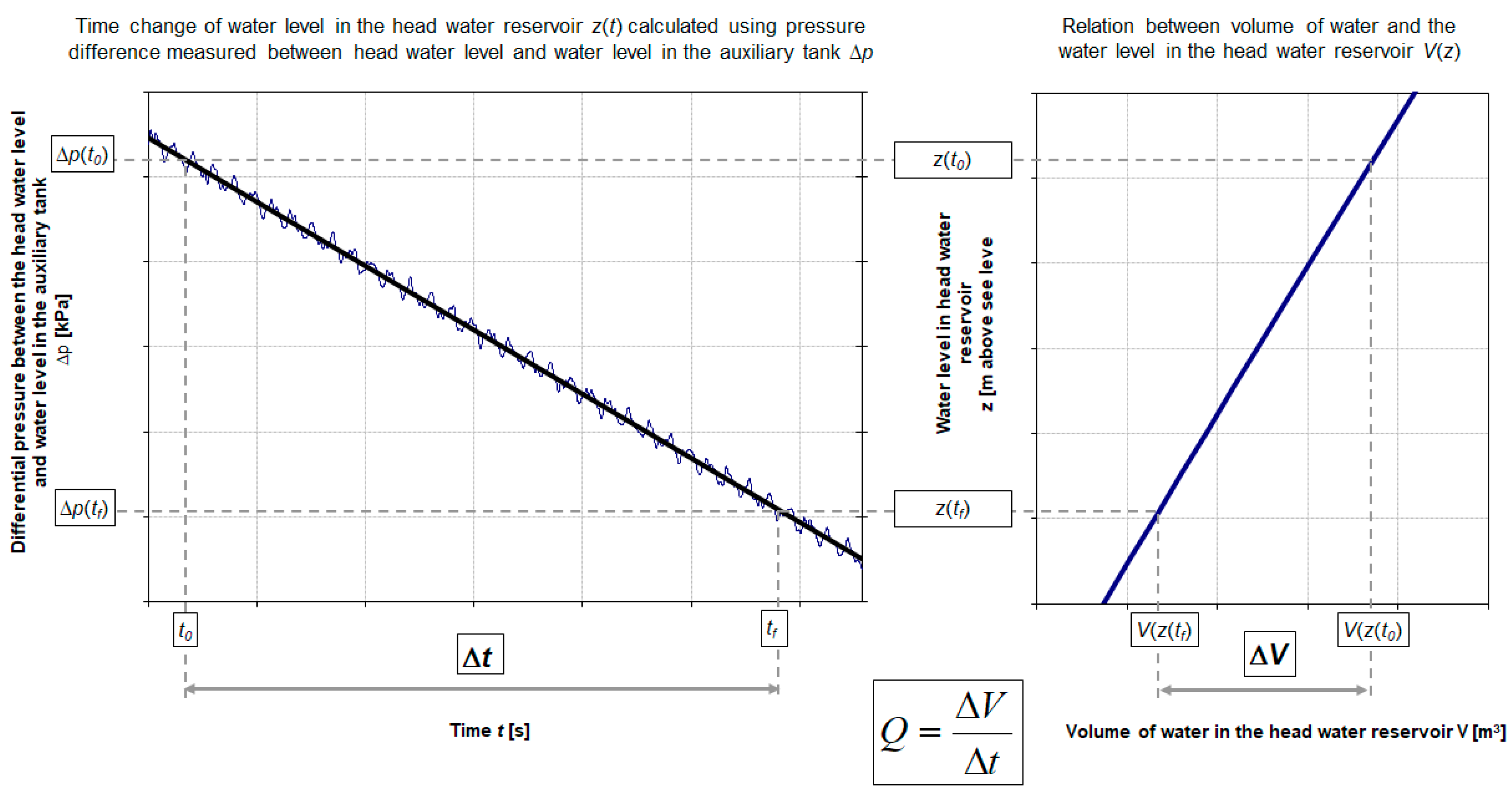
2.2. The Volumetric Gauging Method

Determining discharge using the volumetric gauging method consists in measuring the volume of water ΔV flowing through the tested hydraulic machine during time Δt. The discharge is determined using of the following formula:

$$Q_V=\frac{\mathsf{\Delta }V}{\mathsf{\Delta }t}=\frac{V\left(z\left(t_f\right)\right)-V\left(z\left(t_0\right)\right)}{t_f-t_0}$$

(1)

where ΔV [m³] stands for measured increase or decrease in volume of water in the head water reservoir, $\Delta t=t_f-t_0$ [s]—the time interval in which the increase/decrease in water volume occurred, and z—level of water in the head reservoir.

When using the volumetric gauging method, there are several issues that can significantly affect the accuracy of the measured flow rate [11,18]. The main task is to determine the relationship between the volume and the water level of the reservoir V(z). This relationship should be determined on the basis of precise reservoir geometry measurements (particularly useful for artificial reservoirs) or accurate bathymetric scanning. The issue of determining the reservoir volume also involves measuring the water level in this reservoir.

In common situations, transmitters designed to control this level usually included in the power plant equipment are not suitable for use in the volumetric gauging method as they have a wide measuring range and low accuracy class. In order to achieve low uncertainty of measurements, the change in the water level in the reservoir should be determined using special methods. The schematic diagram of the proposed method is shown in Figure 2. Its most important element is measuring the increase in water level Δz in the power plant reservoir by means of a precise transducer measuring the pressure difference in the reservoir and a constant pressure level set using small auxiliary tank, hung at the appropriate height. The configuration of such an installation should ensure the possibility of carrying out an approximately one-hour measurement at a fixed operating point of the tested hydrounit.

The proposed method allows for the significant reduction of the measurement uncertainty giving an additional possibility for taking into account the unfavorable phenomenon of water surface waving occurring during the tests. This phenomenon can affect the results of the measured flow rate in the most significant way. Traditional ways for measuring the water level used in the volumetric gauging method cannot ensure required accuracy of discharge measurements. Using a measuring system with appropriate characteristics and applying linear regression for the results of measuring the level of water in the reservoir leads to eliminate the effect of water waving on measurement results (Figure 3). It’s worth pointing out that it is very important to base the regression line on the boundaries selected at the extreme points of the peaks or valleys of the differential pressure signal. This is a prerequisite for obtaining the correct final flow measurement results.

Owing to the solutions applied, a very narrow uncertainty range was possible to achieve and the results of its estimation are presented in the next chapter of the paper. The uncertainties (standard and expended) were estimated according to the procedure described in Appendix B that was developed basing on the general recommendations presented in [19].

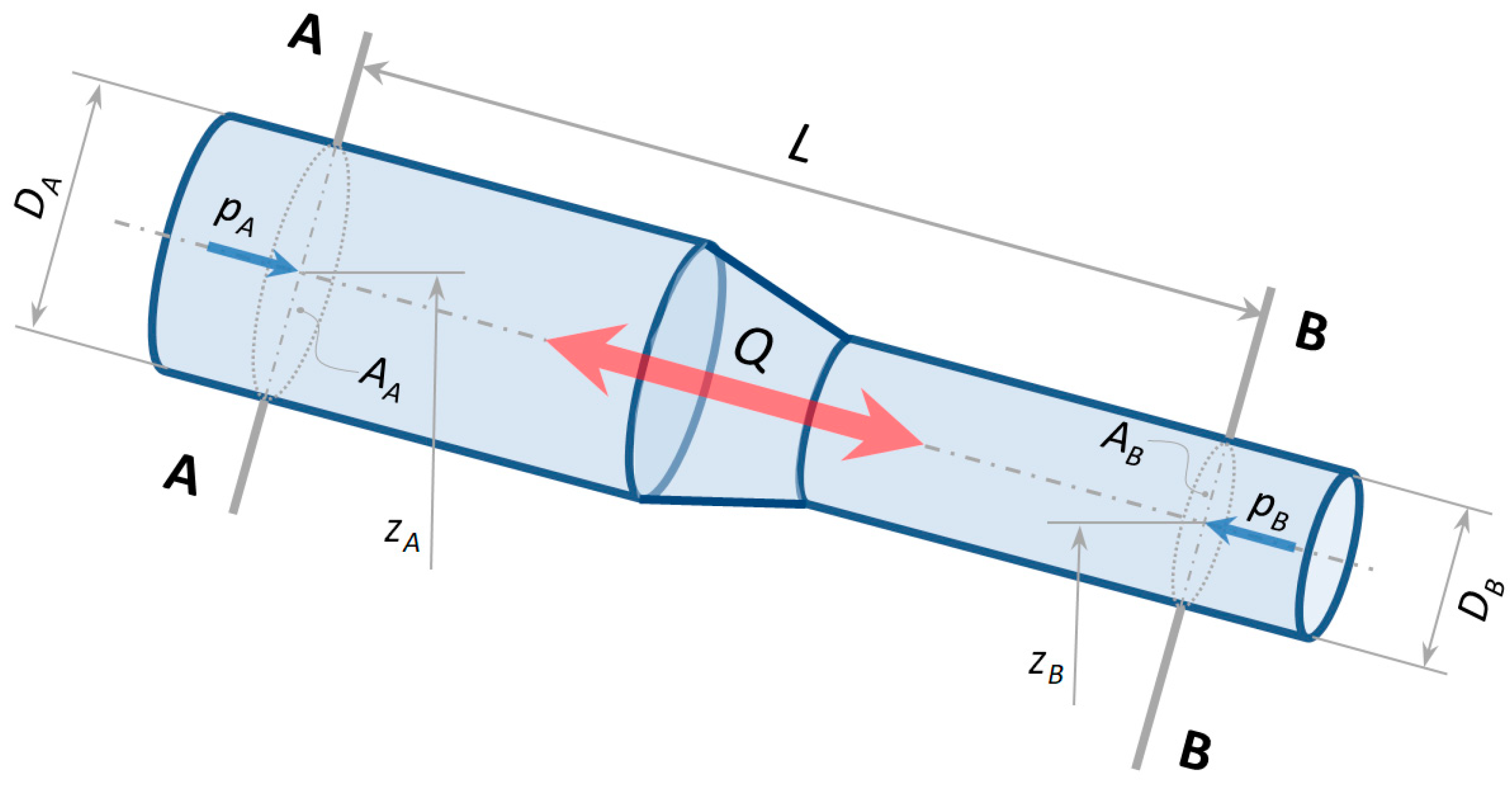
2.3. The Pressure-Time Method

2.3.1. Basic Information

The pressure-time method is based on the relationship between flow rate at steady state conditions and pressure-time change occurring in the pipeline during cutting off the flow [7,8]. The value of Q₀ indicating the discharge at initial liquid flow conditions is calculated using the definite integral over a time interval in which the flow varies from initial conditions to conditions after the flow is completely shut off [4,6,11]:

$$Q_0=\frac{1}{\rho F}\underset{t_0}{\overset{t_f}{{\displaystyle \int }}}\left(\Delta p\left(t\right)+\Delta p_d\left(t\right)+\Delta P_r\left(t\right)\right)\mathrm{d}t+Q_f$$

(2)

where:

ρ is the density of a liquid,

t₀ and t_f are the initial and final time-limits of integration, respectively,

Q_f is the discharge under final steady-state conditions (after complete closing of the shut-off device) due to the leakage through the closed shut-off device,

Δp is the difference in pressures measured between the pipeline measuring cross-sections B-B and A-A, which geometrical centers are at level z_A and z_B, respectively (Figure 4):

$$\Delta p=p_B+\rho g{z}_B-p_A-\rho g{z}_A$$

(3)

Δp_d is the difference in dynamic pressures between the pipeline measuring cross-sections with area of each section equal A_A and A_B:

$$\Delta p_d={\alpha }_2\frac{\rho Q^2}{2A_B^2}-{\alpha }_1\frac{\rho Q^2}{2A_A^2}$$

(4)

where:

α₁, α₂ are the kinetic energy correction factors for A-A and B-B sections (the value of the kinetic energy correction factor for fully developed turbulent flow in the pipeline, dependent on Re number is within the limits from 1.03 to 1.11 [20,21]);

ΔP_r is the pressure loss caused by hydraulic resistance in pipeline between the measurement cross-sections—quantity calculated as proportional to the square of flow rate (accounting for its direction):

$$\Delta P_r=C_r·Q\left|Q\right|$$

(5)

One of the most important parameters in Formula (2) is the F factor. Its value depends on the geometry of the pipeline flow system between the pressure measurement cross-sections. The following formula can be used to calculate the F factor in case of the pipeline segment with length L and j sub-segments with different sizes:

$$F=\underset{0}{\overset{L}{{\displaystyle \int }}}\frac{\mathrm{d}x}{A\left(x\right)}={\displaystyle \sum }_{j=1}^{j=J}\frac{\Delta x_j}{A_j}, \mathrm{with}{\displaystyle \sum }_{j=1}^{j=J}\Delta x_j=L$$

(6)

where Δx_j and A_j indicate the length and internal cross-sectional area of the j-th sub-segment, respectively. As shown in Equation (2), the pressure loss, ΔP_r, representing hydraulic resistance and the dynamic pressure difference, Δp_d, should be separated from the pressure difference measured between the pipeline measurement cross-sections, Δp. In total, the integral expression of Equation (2) defines the pressure difference resulting from the inertia force of the mass of liquid retained in the pipeline measuring section (segment). The values of ΔP_r and Δp_d can be calculated with good accuracy using their dependence on the square of the flow rate in the forms written in Equation (4) and (5).

Measurements made using the pressure-time method, as was the case concerning the volumetric gauging method, were carried out for both flow directions through a reversible machine equipped with Francis type runner. Measuring flow rate in the pump direction requires appropriate modifications of the pressure-time method to the calculation procedures described in the standards, which were postulated by the authors in earlier publications [11,22,23] and which resulted with formula in Equation (5) (introducing term $Q\left|Q\right|$ instead of $Q^2$).

A comprehensive discussion of some problems related to the computational procedures in the pressure-time method is provided in standards [4,6] as well as in monograph [11]. A description of some important problems related to the use of the pressure-time method for measuring flow rate in hydropower plants can also be found in publications [22,23,24,25,26,27,28,29]. Calculation of friction losses according to the quasi-stationary hypothesis is consistent with the conclusions presented in [30]. It was proved that the modelling of unsteady friction losses has little effect on the course of water hammer in its initial time-phase that is taken into account in the pressure-time method. Nevertheless, it should be emphasized that including the transient nature of friction losses into the calculation method, under certain circumstances, may improve predictions of the pressure-time method as described in [27,28,29].

Several variants of the pressure-time method are used in practice. They differ mainly in methods of measuring the pressure differences between pipeline measurement cross-sections. In the considered case, the pressure-time method was used in the variant based on measuring the pressure changes at the cross-section of the pump-turbine spiral case outlet/inlet and relating these changes to the pressure exerted by the water column from the head water reservoir. This variant requires the determination of the geometric factor F accounting the entire penstock of the tested machine, starting from the inlet section and ending with the outlet/inlet cross-section of the spiral case.

The recommendations of the standards [4,5,6] allow the use of the F factor for straight-axis measuring pipelines of variable diameter (according to the Formula (6), taking into account their geometry). However, in the case of more complex changes in the geometry occurring in the measuring section of the pipeline (changes in the shape of the flow section, changes in the direction of the pipeline axis or branches), there is a need to take into account the influence of these changes on the flow conditions.

Irregular parts (components) of the penstock cause flow disturbances in the form of non-uniform water velocity distribution. This should be taken into account in order to ensure better accuracy of discharge measurement. In the considered case, except for the straight pipe sections with constant internal diameters, the penstock has three elbows (two vertical and one horizontal), a number of short conical sections connecting pipes of different diameters, and two short branches, where one branch remained closed during the tests. In addition, the square cross-section as well as transition section from square to the circular cross-section in the highest part of the penstock had to be taken into consideration. In the previously published work [24], authors presented the procedure, based on CFD, used for correction of F-factor calculated in case of penstocks with elbows. The assumption of equal kinetic energy resulting from the simulated and the uniform water flow velocity distributions in the same flow parts of the penstock was the main, except mass conservation law, theoretical basis for this procedure. In this work, using CFD, an extended procedure was developed and applied to correct the value of the F-factor for the above-mentioned irregular components of the penstock under consideration. The procedure is presented in detail in Appendix A. The selected results of CFD calculations and the F-factor correction for the studied case are presented later in this paper.

2.3.2. CFD Based Correction of Penstock Geometrical Factor

The NUMECA/Hexpress commercial software [31] was used for generating the computational grid representing the penstock geometry (Figure 5). The unstructured grids consisted of hexahedral elements.

For flow calculations, ANSYS/Fluent commercial software was used [32]. The flow was simulated by solving the steady-state Reynolds Average Navier-Stokes (RANS) equations with the k-ω SST turbulence model. Many studies demonstrate the great usefulness of this turbulence model in the calculation of industrial flow systems [33,34]. It’s commonly known that the k-ω SST model integrates advantages of both k- turbulence model and standard k-ω turbulence model [35].

The second-order upwind discretization was used with the SIMPLE scheme of pressure-velocity coupling. Non-dimensional distance from wall Y⁺ was assumed to be in range 1 to 5 according to the used turbulence model. Initialization of calculation was done from all zones limiting the computational domain. The calculations were conducted until all of the residuals (continuity residual, velocity components, turbulent kinetic energy, and specific rate of dissipation) reached values less than 0.001. The parameters for a closure of turbulence model were hydraulic diameter and turbulence intensity. First of them was calculated using formula: D_h = 4A/P [m], in which A is the area and P is the perimeter (hydraulic diameter was 1.654 m at inlet/outlet of lower part the penstock and 30 m at inlet/outlet of upper part of the penstock). The second parameter was calculated using the formula [32]: I = 0.16 Re^(−1/8) in which Re is Reynolds number at inlet or outlet cross-section. At the outlet of the measuring section, constant static pressure was assumed for all calculation cases. The free surface of the reservoir was assumed as a no-slip boundary condition.

The CFD calculations were conducted for four discharge values (20, 25, 30, and 35 m³/s) in the turbine operation modes and for two discharge values (26 and 28 m³/s) in the pump operation modes. The sample of calculation results in the form of water velocity distributions in cross-sections for three chosen flow parts of the penstock were presented in Figure 6, Figure 7 and Figure 8 for both flow directions, for analyzed discharge of 35 m³/s in turbine regime, and 28 m³/s in pump regime.

The CFD simulation results received for the analyzed penstock flow parts (Figure 6, Figure 7 and Figure 8) can be characterized as follows:

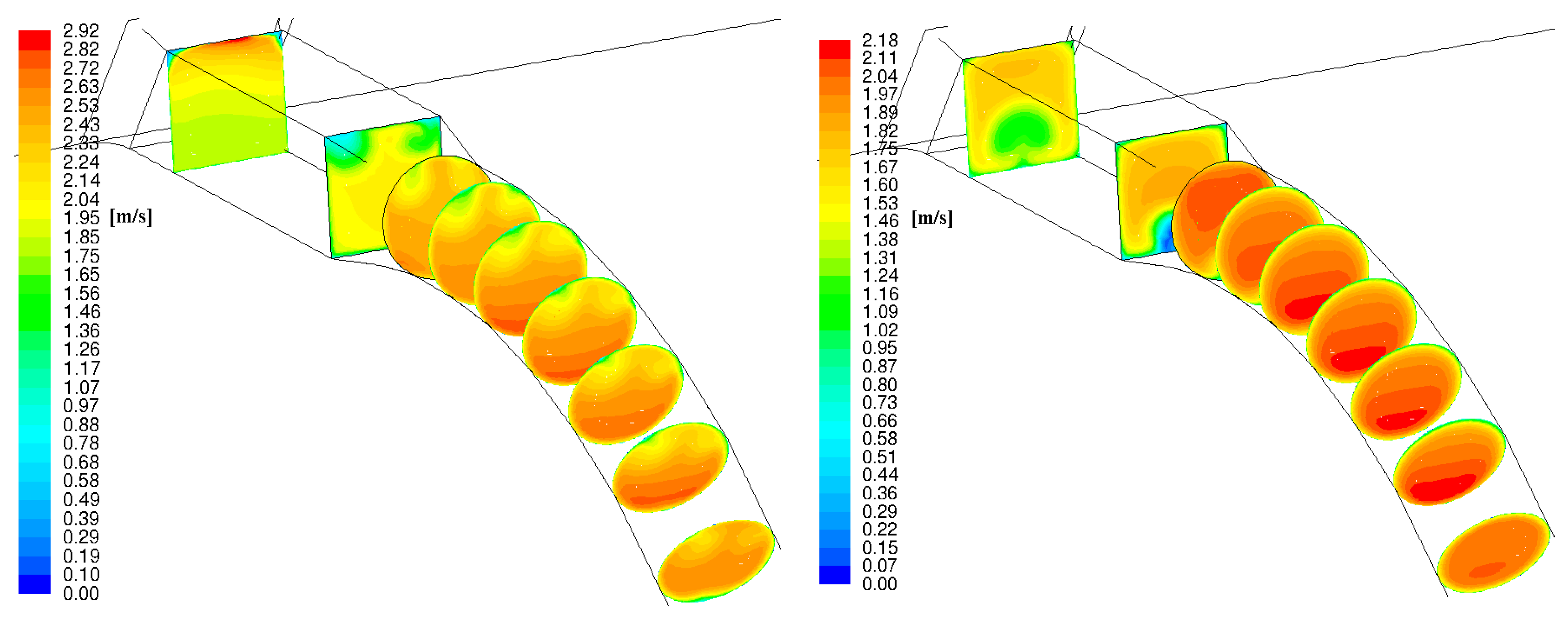
• The water velocity distributions inside the area of the penstock inflow/outflow (in the cross-sections near the head water reservoir) are different for the turbine and pump operation modes.
• The largest irregular flow occurs in the penstock branch and despite the fact that it only affects the velocity distribution locally, the propagation of these irregularities in the direction of the water flow is clearly more visible than in the opposite direction. The intensity of the flow disturbance decreases rapidly with distance. On the other hand, the smallest flow irregularities in the penstock are induced by the existing short tapered pipe sections.
• The velocity distributions in the elbows also differ depending on the direction of flow, which is quite obvious—the elbows induce disturbances in the flow pattern, which propagate to the next penstock components with decreasing intensity. For example, for the turbine operation mode the flow achieving the elbow #2 is almost uniform because of the long straight section of pipe before this elbow (looking in turbine flow direction), while in pump operation mode, a similar effect takes place in elbow #1.

The CFD results taking account flow irregularities induced in the penstock were used to calculate the equivalent factor F_e according to the original procedure presented in Appendix A.

The deviation factor, Δf, representing a relative difference between the equivalent penstock factor, F_e, (obtained using CFD calculations) and the penstock geometrical factor, F, was included in discharge determination according to the pressure-time method. This factor is calculated as follows:

$$\Delta f=\frac{F_e-F}{F}$$

(7)

The values of quantity, Δf, determined for chosen discharge values for both flow directions are presented in

Table 1. The relative differences of F-factor, Δf, determined for the entire penstock for the assumed discharge values in the both machine operation modes.

Machine Operation Mode	Discharge, Q0	Relative Difference of F-Factor, Δf
-	m3/s	%
Turbine operation mode	20	0.15
	25	0.14
	30	0.13
	35	0.11
Pump operation mode	26	0.77
	28	0.77

. It can be stated that Δf is kept almost constant for both flow directions separately. However, it presents different level for both turbine and pump operational modes: the average value of Δf is about +0.13% and about +0.77% for turbine and pump modes of operation, respectively. These values were used as correction quantities of the geometrical factor F calculated based only on the geometry of the entire penstock.

2.3.3. Flow Rate Measurement, Uncertainty

The values of flow rate (discharge) were calculated based on the difference of pressures measured between the inlet/outlet cross-section of the tested pump-turbine (cross-section (B-B)) and the reservoir (cross-section (A-A)) and accounting for F_e factor obtained using CFD. Calculations were carried out using the computer program GIB-ADAM that has been tested and successfully verified on many occasions related to the implementation of laboratory tests as well as e.g., efficiency tests in hydropower plants [11]. Examples of the results measured or calculated for both modes of operation of the pump-turbine under investigation are shown in Figure 9. Measurements begin ca. 30–40 s before shut-off device start closing and end about 30–60 s after its complete closure or after extinction of the free pressure oscillation remaining in the flow system after the flow cut off. The time of closing the wicket gates of the tested machine was about 25 s and 20 s during turbine and pumping mode of operation, respectively. These time intervals were (8–10) times longer than the pipeline pressure wave period of about 2.5 s. Closing of the wicket gates was carried out in two stages in both modes—the faster stage followed by slower one. The reason for this common method of closing the wicket gates is to maintain the safety of the hydraulic system by preventing excessive pressure oscillations caused by too rapid shut-off of the flow, especially in the final phase of wicket gates closing.

The analysis of the influence of the above-mentioned and other parameters on the uncertainty of the results of the flow rate measurement with the applied method is presented in Appendix C.

3. Results and Discussion

The volumetric gauging method of flow measurement, due to the high requirements that must be met, is difficult to apply when testing real objects. For this reason, the examples of its practical application are quite rarely published. More valuable are the results presented in this paper, which were obtained for a pumped-storage power plant equipped with an artificial head water reservoir with known geometric characteristics. This made it possible to use the volumetric gauging method to measure the flow rate through the tested reversible hydrounit. The required narrow uncertainty band was obtained by supplementing the method with a special solution for accurate measurement of the water level change in the reservoir that also allowed including the impact of waves, as well as the amount of rainfall and leaks during measurements. It should be emphasized that measuring the upper water level in a standard way usually cannot ensure sufficient accuracy of the volumetric gauging method used for measuring flow in hydroelectric power plants.

The application of the pressure-time method to measure the flow rate in a real flow system with complex geometry additionally requires the use of an innovative calculation methodology to determine the F-factor—one of the critical parameters for maintaining a sufficiently narrow measurement uncertainty band. Owing to this factor, the geometrical characteristics of a pipeline measuring segment and impact of its flow elements on flow irregularities are taken into account. Disregarding changes in flow velocity profiles resulting from the variable shapes of pipeline elements leads to an increase in the inaccuracy of measurement using the pressure-time method, which cannot be corrected only by improving the modeling of friction losses in these elements, as discussed in [27,28,29] or by improving the computational model [22,28]. In addition, increasing the accuracy of estimation of the leakage rate through closed-flow shut-off devices is not enough [26]. In order to take into account changes in liquid velocity profiles in pipeline bends, the authors proposed a special calculation procedure (described in [24]) using CFD analysis for correction of the F factor. Verification of this procedure based on the analyzed examples confirmed that its application significantly increases the measurement accuracy of the pressure-time method. In this paper, the procedure based on CFD has been extended and used for piping systems with complex geometry (including curves, branches, conical elements, and inlets with changes in the shape of the flow section). In contrast to such a solution, the standard application of the pressure-time method does not provide the required uncertainty of flow rate measurement results. This innovative procedure provides the basis for using the pressure-time method in case of geometrically complex pipelines, and not only in turbine mode of operation, but also in the pump flow conditions of the tested reversible machine.

The uncertainties (standard and expanded) of the flow rate measurement results using both methods under consideration were as follows:

• Volumetric gauging method: standard and extended uncertainties were not greater than +/−0.38% and +/−0.76%, respectively, for all measured flow rates—Appendix B;
• Pressure-time method: standard and extended uncertainties were not greater than +/−1.0% and +/−1.1%, respectively, for all measured flow rates—Appendix C.

3.1. Turbine Operation Mode

Because it was not possible to measure water discharge through the tested machine using both methods (volumetric gauging and pressure-time methods) simultaneously, the comparison of the results measured for the turbine operation mode was performed using the Winter–Kennedy method. According to this method, the measurement of discharge is based on the relationship between the discharge, Q, and the difference of pressures, Δp_wk, between the outer and the inner side of a spiral case of the machine under test:

$$Q=k\Delta p_{wk}^n$$

(8)

where k and n are constant coefficients experimentally determined during the calibration process. A value of the exponent, n, was assumed from the theory as equal to 0.5. Such assumption insignificantly influenced the measuring results as was proven in [17] and it is negligible for purposes of comparison presented in this paper. For the tested machine, the values of k coefficient were determined independently on the basis of discharge measurement conducted using the volumetric gauging and the pressure-time methods—in Figure 10. The difference between k coefficient values obtained using these two different methods is very small, only about 0.2%. It should be emphasized that for the penstock geometric factor, F, used in the pressure-time method without the ∆f correction, the difference in the value of the k coefficient is slightly larger and amounts to approximately 0.33%. Although in the case under consideration the difference is not large, taking into account the various pipeline geometries that encounter in practice, it is recommended to support the pressure-time method by means of CFD analysis in the case of measuring sections of pipelines with irregular elements causing disturbances in the flow.

3.2. Pumping Operation Mode

The use of the Winter–Kennedy method for measuring flow rate in the pump mode of operation of hydraulic machines is not recommended by the standards [4,5,6]. This made it impossible to compare the pressure-time and volumetric gauging methods in a manner analogous to that used for turbine mode of operation, i.e., based on the results of simultaneous flow measurements. The comparison of results obtained using the analyzed methods was made by referring them to the head of the plant—Figure 11. The analysis also covered the impact of the penstock geometry irregularities on the results obtained using the pressure-time method. The differences between the discharge results obtained from the volumetric gauging method and pressure-time method were from −0.16% to +0.58% for lower (426 m) and higher head (439 m), respectively. Without correction of F geometrical factors, the differences were much greater—their values were +0.6% and +1.35%, correspondingly.

The comparison shows that the differences between the results obtained using the analyzed methods are much larger for pump mode of operation than for turbine mode of operation. At this stage of research, the causes of such observations cannot be clearly explained. Measurement of the hydraulic machine discharge using the pressure-time method is much more difficult to perform in pump operation than in turbine operation. This fact may suggest the reasons for this comparison results. This may also be the main reason why current standards do not recommend using this method in pump mode of operation of tested machines. However, it should be emphasized that the differences obtained in the analyzed case are still within the range of the measurement uncertainty characterizing the compared methods.

In addition, it should be emphasized that between the pump and turbine modes, in addition to obvious differences, there are those that can significantly affect the results obtained using the pressure-time method:

• Shutoff during pumping is characterized by much more irregular pressure changes than when cutting off flow during turbine mode of operation. This is related to the fact that during turbine operation, the flow was cut off while maintaining the generator connected to the network, while in pump operation, complete flow cut-off with the motor connected to the network was unacceptable.
• At the final stage of closing the machine’s wicket gates, during pump operation, there is a short change in the direction of fluid flow—from the pump to the turbine direction;
• Due to the direction of flow, it should be noted that the pump operation mode, in contrast to the turbine operation mode, induces pressure pulsations with a much higher level, which propagate along the pipeline and have a direct impact on the measured pressure difference.
• The flow in the pump direction takes place along the expanding flow elements of the pipeline (diffusers), which is the reason for greater hydraulic losses (pressure losses occur due to local losses caused by greater turbulence in the boundary layers) and as a result requires greater correction of the F geometrical factor compared to turbine flow (and flow through the confusors).

Precise identification of how these differences may affect the final accuracy of flow measurement results obtained with the pressure-time method in the pump mode of operation of the hydraulic machines requires thorough professional testing and analysis. Currently, there is insufficient data on this topic, which hinders the extension of the applicability of this method and can also lead to excessive simplifications resulting in increased measurement uncertainty.

4. Conclusions

The paper presents experiences concerning the use of the volumetric gauging method and the pressure-time method for measuring the water discharge through a reversible hydraulic machine at a pumped storage power plant. Research using these methods concerned both turbine and pump mode of operation of the tested machine. As part of the research, new original procedures have been used aimed at significant reduction of the measurement uncertainty.

In the case analyzed in the article by appropriate treatment consisting of the use of high-quality transducers, with the use of appropriate measurement techniques and procedures supporting the measurements of the flow rate with the use of both methods, a satisfactorily low measurement uncertainty was achieved.

The use of a high-class transducer measuring the pressure difference between the upper reservoir and the auxiliary tank in the volumetric gauging method, as well as the original method of analysis of the measured pressure difference, allowed to increase the accuracy of measuring the change in water volume over time significantly, and also allowed us to take into account water waving, which, when ignored, can meaningly distort measurements.

The pressure-time method, which required taking into account the complex geometry of the pipeline connected to the tested hydrounit, was supported by CFD analysis of flow in the area of geometric irregularities (inlet, diameter changes, elbows, changes in cross-sectional shape). The original procedure using the results of this analysis provided the information necessary to introduce appropriate adjustments (correction) to the geometric factor F, which in turn, contributed to a significant reduction in the flow rate measurement uncertainty.

In contrast to the very good compliance of the results of discharge measurements obtained with the analyzed methods for the turbine operation of the tested machine (differences in the range of ±0.2%), in the case of pump operation, larger differences between the results were observed; however, they were still in the uncertainty band for measuring each of these methods independently (differences from −0.16% to +0.58%). At this stage, it is difficult to clearly explain these observations. The authors point out the differences in the course of flow phenomena during shut-off in turbine and pumping operation carried out as part of tests executed using the pressure-time method. There is a need for further research to explain the reasons of the obtained differences and their influence on the accuracy of discharge measurement using the pressure-time method in pump operation mode.

It is worth emphasizing the positive effect achieved by using the CFD procedure to support the pressure-time method. A measure of this effect is the reduction of the differences between the measurement results obtained using the volumetric gauging method and the pressure-time method. In the turbine operation mode, the CFD-based correction of the F factor resulted in a 1.5-fold increase in the convergence of the compared results. In the case of pumping mode of operation, the convergence has improved several times (more than 2- to almost 5-fold, depending on the point of operation). This result proves the correctness of the assumptions made when using the CFD procedure and using its results for the pressure-time method of measuring the flow.

Particularly noteworthy are the results obtained for the pumping mode of operation, for which the use of the pressure-time method is not recommended by the standards. The comparison and consistency of these results with the results obtained with the volumetric gauging method confirmed the correctness of the assumptions underlying the proposed and applied modifications to the calculation procedure of the pressure-time method. This includes also the correct consideration of the temporary change in the flow direction occurring during its cutting off in the pumping mode of operation. Such experience from using this method in practice can help working out the relevant changes in the standards leading to the recommendation of the pressure-time method also for the pumping mode of reversible hydraulic machine operation.

References

1. Merzkirch, W. Fluid Mechanics of Flow Metering; Merzkirch, W., Ed.; Springer: Berlin/Heidelberg, Germany; New York, NY, USA, 2005; ISBN 3-540-22242-1. [Google Scholar]
2. Miller, R.W. Flow Measurement Engineering Handbook, 3rd ed.; McGraw-Hill Book Company: New York, NY, USA, 1996. [Google Scholar]
3. Urquiza, G.; Basurto, M.A.; Castro, L.; Adamkowski, A.; Janicki, W. Flow measurement methods applied to hydro power plants, Chapter 7. In Flow Measurement; Urquiza, G., Castro, L., Eds.; INTECH Open Access Publisher: Rijeka, Croatia, 2012; pp. 151–168. [Google Scholar]
4. Field Acceptance Tests to Determine the Hydraulic Performance of Hydraulic Turbines, Storage Pumps and Pump-Turbines; IEC 41:1991; European Equivalent: EN 60041:1999; International Electrotechnical Commision: Geneva, Switzerland, 1991.
5. Hydraulic Machines—Acceptance Tests of Small Hydroelectric Installations; IEC 62006:2010; European Equivalent: EN 62006:2011; International Electrotechnical Commision: Geneva, Switzerland, 2010.
6. Hydraulic Turbines and Pump-Turbines. Performance Test Codes; ASME PTC 18 Standard; The American Society of Mechanical Engineers: New York, NY, USA, 2011.
7. Gibson, N.R. The Gibson method and apparatus for measuring the flow of water in closed conduits. ASME Power Div. 1923, 45, 343–392. [Google Scholar]
8. Gibson, N.R. Experience in the use of the Gibson method of water measurement for efficiency tests of hydraulic turbines. ASME J. Basic Eng. 1959, 81, 455–487. [Google Scholar] [CrossRef]
9. Voser, A.; Bruttin, C.; Prénat, J.-E.; Staubli, T. Improving acoustic flow measurement. Water Power Dam Constr. 1996, 48, 30–34. [Google Scholar]
10. Lüscher, B.; Staubli, T.; Tresch, T.; Gruber, P. Accuracy analysis of the acoustic discharge measurement using analytical, spatial velocity profiles. In Proceedings of the Hydro 2007, Granada, Spain, 15–17 October 2007. Paper 17.05. [Google Scholar]
11. Adamkowski, A. Discharge measurement techniques in hydropower systems with emphasis on the pressure-time method. Chapter 5. In Hydropower–Practice and Application; Hossein, S.-B., Ed.; INTECH Open Access Publisher: London, UK, 2012; pp. 83–114. [Google Scholar]
12. Doering, J.C.; Hans, P.D. Turbine discharge measurement by the velocity-area method. J. Hydraul. Eng. 2001, 127, 747–752. [Google Scholar] [CrossRef]
13. Gandhi, B.K.; Verma, H.K. Simultaneous multi-point velocity measurement using propeller current meters for discharge evaluation in small hydropower stations. In Proceedings of the International Conference on Small Hydropower Hydro Sri Lanka, Kandy, Sri Lanka, 22–24 October 2007. [Google Scholar]
14. Proulx, G.; Cloutier, E.; Bouhadji, L.; Lemon, D. Comparison of discharge measurement by current meter and acoustic scintillation methods at La Grande-1. In Proceedings of the IGHEM, Luzern, Swiss, 14–16 July 2004. [Google Scholar]
15. Llobet, J.V.; Lemon, D.D.; Buermans, J.; Billenness, D. Union Fenosa Generación’s field experience with Acoustic Scintillation Flow Measurement. In Proceedings of the IGHEM, Milan, Italy, 3–6 September 2008. [Google Scholar]
16. Adamkowski, A.; Janicki, W.; Krzemianowski, Z.; Lewandowski, M. Volumetric gauging method vs Gibson method—Comparative analysis of the measurement results of discharge through pomp-turbine in both operation modes. In Proceedings of the IGHEM 2016, Linz, Austria, 24–26 August 2016; p. 567. [Google Scholar]
17. Adamkowski, A.; Lewandowski, M. Some experiences with flow measurement in bulb turbines using the differential pressure method. IOP Conf. Ser. Earth Environ. Sci. 2012, 15, 062045. [Google Scholar] [CrossRef]
18. Adamkowski, A.; Lewandowski, M.; Lewandowski, S.; Cicholski, W. Calculation of the cycle efficiency coefficient of pumped-storage power plant units basing on measurements of water level in the head (tail) water reservoir. In Proceedings of the 13th International Seminar on Hydropower Plants, Vienna, Austria, 24–26 November 2004. [Google Scholar]
19. Uncertainty of Measurement—Part 3: Guide to the Expression of Uncertainty in Measurement; (GUM: 1995), ISO/IEC GUIDE 98-3:2008; International Organization for Standarization: Geneva, Switzerland, 2008.
20. Çengel, Y.A.; Cimbala, J.M. Fluid Mechanics. Fundamentals and Applications; McGraw-Hill Book Company: New York, NY, USA, 2006. [Google Scholar]
21. White, F.M. Fluid Mechanics; WCB/McGraw-Hill: Boston, MA, USA, 1999. [Google Scholar]
22. Adamkowski, A.; Janicki, W. Elastic water-hammer theory–based approach to discharge calculation in the pressure-time Method. J. Hydraul. Eng. 2017, 143, 06017002. [Google Scholar] [CrossRef]
23. Adamkowski, A.; Janicki, W.; Krzemianowski, Z.; Lewandowski, M. Flow rate measurements in hydropower plants using the pressure-time method—Experiences and improvements. Flow Meas. Instrum. 2019, 68, 101584. [Google Scholar] [CrossRef]
24. Adamkowski, A.; Krzemianowski, Z.; Janicki, W. Improved Discharge Measurement Using the Pressure-Time Method in a Hydropower Plant Curved Penstock. ASME J. Eng. Gas Turbines Power 2009, 131, 053003. [Google Scholar] [CrossRef]
25. Adamkowski, A.; Janicki, W. Selected problems in calculation procedures for the Gibson discharge measurement method. In Proceedings of the IGHEM, Roorkee, India, 21–23 October 2010; pp. 73–80. [Google Scholar]
26. Bortoni, E.C. New developments in Gibson’s method for flow measurement in hydro power plants. Flow Meas. Instrum. 2008, 19, 385–390. [Google Scholar] [CrossRef]
27. Jonsson, P.P.; Ramdal, J.; Cervantes, M.J. Development of the Gibson method—Unsteady friction. Flow Meas. Instrum. 2012, 23, 19–25. [Google Scholar] [CrossRef]
28. Dunca, G.; Iovănel, R.G.; Bucur, D.M.; Cervantes, M.J. On the Use of the Water Hammer Equations with Time Dependent Friction during a Valve Closure, for Discharge Estimation. J. Appl. Fluid Mech. 2016, 9, 2427–2434. [Google Scholar] [CrossRef]
29. Sundstrom, L.R.J.; Saemi, S.; Raisee, M.; Cervantes, M.J. Improved frictional modeling for the pressure-time method. Flow Meas. Instrum. 2019, 69, 101604. [Google Scholar] [CrossRef]
30. Adamkowski, A.; Lewandowski, M. Experimental Examination of Unsteady Friction Models for Transient Pipe Flow Simulation. ASME J. Fluids Eng. 2006, 128, 1351–1363. [Google Scholar] [CrossRef]
31. NUMECA International—Computational Fluid Dynamics Software and Consulting Service. Available online: https://www.numeca.com (accessed on 15 August 2020).
32. ANSYS Inc. ANSYS Fluent User’s Guide 18; Release 18; ANSYS Inc.: Canonsburg, PA, USA, 2017. [Google Scholar]
33. Menter, F.R. Two-equation eddy-viscosity turbulence models for engineering applications. AIAA J. 1994, 32, 269–289. [Google Scholar] [CrossRef] [Green Version]
34. Wilcox, D.C. Turbulence Modeling for CFD; DCW Industries, Inc.: La Canada, CA, USA, 1993. [Google Scholar]
35. Hellsten, A.; Laine, S. Extension of the k-ω-SST Turbulence Models for Flows over Rough Surfaces; AIAA Paper; AIAA-97-3577; AIAA: Reston, VA, USA, 1997. [Google Scholar] [CrossRef]
36. Ramdal, J.; Jonsson, P.P.; Dahlhaug, O.G.; Nielsen, T.K.; Cervantes, M. Uncertainties for pressure-time efficiency measurements. In Proceedings of the IGHEM 2010, Roorkee, India, 21–23 October 2010; pp. 64–72. [Google Scholar]
37. Hulås, H.; Dahlhaug, O.G. Uncertainty analysis of Pressure-Time measurements. In Proceedings of the IGHEM 2006, Portland, OR, USA, 30 July–1 August 2006; pp. 1–13. [Google Scholar]
38. Brunone, B.; Golia, U.M.; Greco, M. Some Remarks on the Momentum Equations for Fast Transients. In Proceedings of the 9th Round Table, IAHR, International Meeting on Hydraulic Transients with Column Separation, Valencia, Spain, 4–6 September 1991; pp. 201–209. [Google Scholar]
39. Bughazem, M.B.; Anderson, A. Problems with Simple Models for Damping in Unsteady Flow. In Proceedings of the International Conference on Pressure Surges and Fluid Transients, BHR Group, Harrogate, UK, 16–18 April 1994; pp. 537–548. [Google Scholar]
40. Vitkovsky, J.P.; Lambert, M.F.; Simpson, A.R.; Bergant, A. Advances in Unsteady Friction Modeling in Transient Pipe Flow. In Proceedings of the 8th International Conference on Pressure Surges, The Hague, The Netherlands, 12–14 April 2000; pp. 471–482. [Google Scholar]
Figure 1. Flow system of the pump-turbine.
Energies 13 04706 g001
Figure 2. The water level change measurement technique used in the volumetric gauging method.
Energies 13 04706 g002
Figure 3. The volumetric gauging method—basic rules of flow rate determination.
Energies 13 04706 g003
Figure 4. Scheme of the penstock measuring section with markings.
Energies 13 04706 g004
Figure 5. Geometry of hydraulic system (calculation domain): head water reservoir (hydraulic diameter of virtual half-cylindrical inlet 30 m) → square pipeline (4.3 × 4.3 m) → cylindrical pipe (4.3 m) → conical pipe (4.3/3.9 m) → cylindrical pipe (3.9 m) → conical pipe (3.9/3.6 m) → cylindrical pipe (3.6 m) → conical pipe (3.6/3.2 m) → cylindrical pipe (3.2 m) → pipe branch for two pump-turbines (2.276 m) → conical pipe (2.276/1.654 m) → outlet cylindrical pipe (1.654 m)).
Energies 13 04706 g005
Figure 6. The water velocity contours in the penstock inlet part with first elbow for discharge of Q = 35 m3/s in turbine regime (left view) and for discharge of Q = 28 m3/s in pump regime (right view).
Energies 13 04706 g006
Figure 7. The water velocity contours in the penstock part containing the cone pipe for discharge of Q = 35 m3/s in turbine regime (left view) and for discharge of Q = 28 m3/s in pump regime (right view).
Energies 13 04706 g007
Figure 8. The water velocity contours in the penstock part containing the pipe branch for discharge of Q = 35 m3/s in turbine regime (left view) and for discharge of Q = 28 m3/s in pump regime (right view).
Energies 13 04706 g008
Figure 9. Examples of measured values of wicket gates opening and pressure difference and discharge through the machine calculated using the pressure time method. Left view: turbine operation mode, right view: pump operation mode.
Energies 13 04706 g009
Figure 10. Turbine operation mode of the tested hydrounit: Comparison of the volumetric measurement method and the pressure-time method based on the results of calibration of the technical installation of the Winter–Kennedy method, with which the tested pump-turbine was equipped.
Energies 13 04706 g010
Figure 11. Pump operation mode of the tested hydrounit: Comparison of the discharges measured by the volumetric gauging method and the pressure-time method.
Energies 13 04706 g011