Energy-Based Vibration Modeling and Solution of High-Speed Elevators Considering the Multi-Direction Coupling Property

Abstract

Vibration of a high-speed elevator is one of the major factors contributing to a safe, stable and comfortable ride. Vibration control and systematic optimization rely on the establishment of an accurate and reliable model. An energy-based vibration model (EVM) is proposed in this paper to describe the multi-directional coupling properties of high-speed elevators. After analyzing the structural and kinematic characteristics, a combination of the kinematic energy, elastic potential energy and virtual works is implemented to describe the vibrational characteristics. The Gaussian precise integration method is implemented to obtain accurate solutions because of the infinite degrees of freedom and the time-varying parameters. An example study is conducted using the KLK2 high-speed elevator. EVM is established to obtain the $Max(P_k)/P_k$ and A95 indices of the X, Y, Z axis vibrational acceleration through simulations. A comparison is proposed between the proposed EVM method, conventional methods based on differential-equation vibration model (DVM) and real prototype experimental data. Results show that the proposed EVM method could achieve more accurate results than the conventional DVM method. Deviations of these indicators are less than 5%, which suggest the efficiency, precision and reliability of the proposed EVM.

1. Introduction

Operating speed and lifting elevation have been rapidly increasing with the high-rise buildings springing up. Generally, many causes, including installation error of the guide rail, stretch of the traction rope, airflow disturbance in the lift well and systematic intrinsic frequency, have impacts on the vibration of the lift car, which would significantly affect riding comfortability and safety. Vibration analysis, control, reduction and optimization of high-speed elevators demand a comprehensive solution urgently, which have attracted attention in the past few decades.

Vibration modeling and simulation techniques of high-speed elevators have constructed a solid theoretic basis in the literature. Through analysis on the non-linear vibration property of a moving elevator string with a weighted end, a time-varying differential equation set was constructed in [1], and further approximately solved by Hamilton’s principle. The natural frequency and modes of the elevator traction system were analyzed in [2] after applying external excitation. The free vibration equation is constructed based on the obtained response characteristics, and were applied in normal operation and emergency braking tests. To avoid the potential danger caused by the natural frequency coincidence between the high-rise building and the traction rope, a comprehensive mathematical model is presented in [3] considering the combined lateral stiffness of the guiding system. Also targeting at the influence of the lateral vibration on the dynamic response of traction rope, a vibration model was derived in [4] with quadratic and cubic non-linear terms. Further, the influence of cage motion and rope stretch were also considered in [5] to construct a dynamic model for both vibration analysis and prediction. Modal analysis in the operating condition is conducted in [6] for stiffness coefficients estimation through minimizing the summed mode shape and frequency errors between the experiments and the analytical model. A forced vibration differential equation was proposed in [7,8] to model the non-linear characteristics of the rolling guide shoes in consideration of the random perturbation of the guide rails and uncertainty of the car parameters. Then, horizontal vibration response of the car is proved to be influenced by the irregularity of the guide rails. The nonlinear behavior between the guide roller and the guiding rails was observed and investigated in [9]. Subsequently, a mathematical method along with an efficient parameter estimation method was proposed. Considering the combined effect of the guide rail perturbation and air flow disturbance, a transverse vibration model with four degrees of freedom is proposed in [10] based on computational fluid dynamic analysis under different working conditions. An adaptive vibration model based on neural network was proposed in [11] for vibration estimation, evaluation and prediction. An active roller guide system was developed and fully researched in [12] to prove its outstanding performance of controling elevator vibration and reducing electric power consumption. The nonlinear oscillation and stability of the elevator was investigated in [13], and an analytical solution based on parameter expansion was provided after estimating the influence of different parameters on the systematic response.

Some existing researches have focused on vibration optimization and control techniques. Vibration cannot be eliminated totally and thoroughly, but could be controlled and reduced to increase riding comfortability for passengers. A reduced order control model of the ultra high speed elevator was generated in [14], and the performance was proved through numerical simulations. Lateral vibrations of the traction rope caused by wind perturbation were studied in [15] considering the rope stretch, with the assumption that the axial, vertical velocity was treated constant. A specially designed input device with gaps installed near the upper end of the traction rope was proved to be efficient and robust in vibration control of the elevator [16]. A new control suppressor presented in [17] made use of the control force and actuator stroke to suppress vibration. The efficiency of controlling the first and second mode lift car vibration has been proved. Position of the installed vibration suppressor was researched in [18] to obtain the actual resonant position. Finite difference analysis with or without vibration suppressor were conducted for comparison. Based on test results of acceleration responses performed on an experimental elevator model, a non-stationary mathematical model was generated in [19]. The parameters were obtained through the Finite Element Method. A vibration control strategy based on the state-dependent Ricatti equation was proposed in [20] to suppress the horizontal nonlinear behavior after investigating the tilting motion of the lift car. A control device composed of two rotary electric motors was proposed in [21] to limit the irregular horizontal motion of the lift car on the guide rail, while not introducing any additional vertical vibration. An active suspension system was developed and verified in [22,23] which is composed of six actuators to suppress the horizontal vibrations. To suppress the lateral vibration, an active roller guide system was proposed in [24,25] with significant advantages of controlling performance and electric consumption. It was observed in [26], that the fundamental vibration frequency of the front-back direction is lower than the lateral direction. The necessity of considering the coupling effect from both directions was emphasized. An innovative method of vibration control was proposed in [27] through optimizing the number of poles slots of a gearless elevator system. An extended full-order observer configuration was introduced in [28] to obtain a systematic observation simultaneously, based on which an acceleration feed compensation was implemented. Sway and stretch of both ropes were controlled in [29] while treating the systematic natural frequency and damping ratio as time varying parameters. Based on investigations on the nonlinearities of the horizontal response under rail perturbations, a linear quadratic regulator control strategy along with a magnetorheological damper was developed in [30] to adjust the control force while considering parametric errors and measurement noises. Numerical simulations were then implemented to verify the effectiveness and robustness in improving driving comfort.

Based on the kinematic differential equations, researches in the literature have reduced the impact of vibration on riding comfortability through optimizing design parameters and developing vibration reduction devices. Establishment of a comprehensive vibrational model would construct the theoretic basis of subsequent analysis for vibration patterns, influencing factors, and vibration-control-oriented optimization. Traditionally, vertical [28,31,32] and horizontal [20,33,34] vibrations are treated separately. The coupling effect has not been taken into account properly. The mass of the traction rope is usually neglected, which would cause damage to the modeling reliability because of its significant length. In addition, the commonly used partial differential equation sets have unlimited degrees of freedom, which makes it difficult to obtain accurate solutions. The uncertainty and complexity of external perturbances would lower the accuracy and reliability of vibration models formulated by kinematic differential equations.

As a solution, an energy-based vibration model (EVM) is established in this paper to describe the multi-direction coupling vibration property of high-speed traction system. Through a combination of the kinematic energy, elastic potential energy and damping virtual work, the mass of the traction rope is considered and the uncertain perturbances are avoided. Computational accuracy is promoted through the implementation of Gaussian precise integration method. A real example is analyzed using KLK2 high-speed elevator of a known manufacturer. The EVM is constructed to compute key indicators $Max(P_k)/P_k$ and $A95$ of vibrational acceleration along X, Y, and Z axis. Finally, a comparison is shown between results obtained by EVM, traditional differential-equation vibration model (DVM) and a prototype. Solution results and experimental data on KLK2 prototype have shown the established EVM is more effective and efficient than the conventional DVM.

2. Structural and Vibrational Characteristics

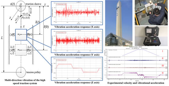
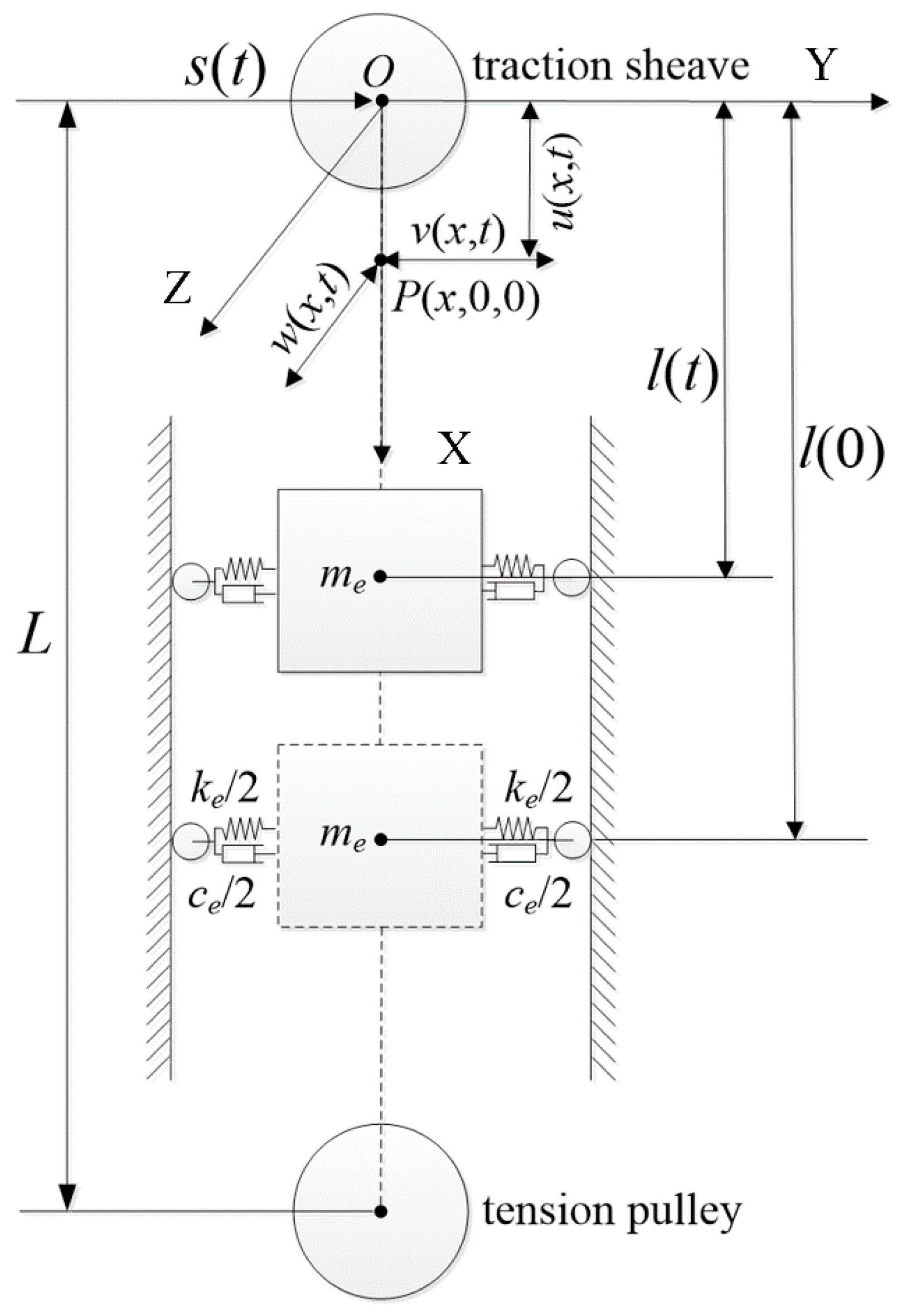
2.1. Basic Structure of a High-Speed Traction System

The mechanical structures of high-speed traction systems are varied according to their designed speed and load capacity. One of the most commonly used structure is shown in Figure 1, in which some principle parts including the traction sheave, lift car, traction rope, rope tension device, guiding pulley and compensation rope are presented. The lift car is driven up and down by the friction effect between the traction sheave grooves and the traction rope. Connecting the lift car and the counterweight, the traction rope bears a position and time-varying axial tension and is extended dynamically. The high-speed traction system is a typical slender flexible system.

2.2. Analysis of Multi-Direction Coupling Vibration

In consideration of the traction system, axial stretch and sidewise swing of the traction rope are the direct causes of systematic vibration. To provide a precise description of the multi-direction coupling vibration while reducing computation, the following assumptions are made:

• The impact of the rope stiffness on vibration could be neglected [1,35,36]. The traction rope is simplified to flexible strings.
• Radial deformation scale could be neglected compared with axial stretch. Small elements on the traction rope share the same scalar of velocity, and physical parameters (such as elasticity modulus, linear density) are generally constant.
• The guide rail and the elevator well do not belong to the traction system. Fabrication uncertainties, installation deviation of the guide rail, and airflow of the elevator well are not the direct causes of traction system vibration, which could be simplified as constant perturbations at the contact point between the traction sheave and the rope.
• The traction sheave and the tension pulley are treated as mass points considering the significant dimensional difference between the length of the traction rope and the radius of pulleys. Therefore, the segmented strings are connected at the mass centers of the traction sheave and the tension pulley.

Structural simplification of the high-speed traction system is conducted based on those aforementioned rules. The systematic multi-direction coupling vibration characteristic is shown in Figure 2. Establish the Cartesian coordinate system at the mass center of the traction sheave. The vertical X axis describes the positive traction stretch; the Y axis is horizontal; the direction of the Z axis follows the right-hand rule. The traction rope is segmented to two strings, both of which bear axial tension. The lift car is considered as a rigid object centered $m_e$, which is connected in both ends by the two strings. The impact of hydraulic guiding shoe, which limits the kinematic degree of freedom and provides lubrication, is simulated using a spring-damper system with a stiffness coefficient $k$ and a damper coefficient $c$. $s(t)$ represents an external perturbation along Y axis to simulate one of the actual vibrational sources in consideration of modeling reliability and computational convenience.

Assume the linear density of the traction rope is $\rho$, cross-section area is $S$, and elasticity modulus is $E$. $l(t)$ is used to denote the length of the string at time $t$, and $L$ is used to represent the projection distance along X axis between the traction sheave and the tension pulley. Consider an element $P(x,0,0)$ at distance $x$ away from the spatial origin. The projections of the actual displacements along X, Y and Z axis are respectively represented as $u(x,t)$, $v(x,t)$ and $w(x,t)$. Therefore, the vertical velocity and acceleration of the lift car could be formulated as $v(t)=\dot{l}(t)$ and $a(t)=\dot{v}(t)$ using the differential operation.

3. Vibration Modeling Based on Energy Methods

3.1. Formulations of the Vibration Model Based on Energy Analysis

The vibrational models and the solutions of the traction system are similar regarding the acceleration and deacceleration stages in both height-lifting and height-reducing process. Only the displacement, velocity and acceleration vectors could be opposite in signs. Therefore, in consideration of limited space available, only the deacceleration stage in the height-lifting process is discussed and elaborated in this paper. To construct the vibration model, translation vector of an element $P(x,0,0)$ is formulated as [1,37]:

$$R=\left[x(t)+u(x,t)\right]i+v(x,t)j+w(x,t)k,$$

(1)

where $i$, $j$ and $k$ are used for translational unit vector along X, Y and Z axis respectively. Velocity vector $V$ is then calculated through the deviation operation $D$ on both sides:

$$V=\left[v(t)+\frac{Du(x,t)}{Dt}\right]i+\frac{Dv(x,t)}{Dt}j+\frac{Dw(x,t)}{Dt}k$$

(2)

The deviation operation $D$ is defined by:

$$\frac{D}{Dt}=\frac{\partial }{\partial t}+v(t)\frac{\partial }{\partial x}$$

(3)

$u$, $v$ and $w$ are used to simply record $u(x,t)$, $v(x,t)$, $w(x,t)$, and subscript $e$ is used to mark physical quantities regarding properties of the lift car. The translation vector and velocity vector of the lift car are then obtained:

$$R_e=\left[l(t)+u(l,t)\right]i+v(l,t)j+w(l,t)k$$

(4)

$$V_e=\left[v(t)+\frac{Du(l,t)}{Dt}\right]i+\frac{Dv(l,t)}{Dt}j+\frac{Dw(l,t)}{Dt}k$$

(5)

The kinematic energy of the traction system is formulated in:

$$E_k=\frac{1}{2}{m}_e{V}_e^2+\frac{1}{2}\rho {{\displaystyle \int }}_0^l{V}^{2}dx+\frac{1}{2}\rho {{\displaystyle \int }}_l^H{V}^{2}dx$$

(6)

where the kinematic energy of the lift car, traction string and tension string at time $t$ are included respectively as the first, second and third term in Equation (6).

The traction string bears the gravity and pre-tension of the tension string, as well as the gravity of itself and the lift car. The tension string is only influenced by its gravity and the pre-tension force. The gravity acceleration $g$ is a positive constant scalar quantity along the positive direction of X axis. The static tension of an element $P(x,0,0)$ in the traction string at time $t$ could be formulated as:

$$T(x,t)=\{\begin{array}{c}\left[m+\rho (l(t)-x)\right]g+F(0<x<l^{-}(t))\\ \rho (L-x)g+F(l^{+}(t)<x<L)\hfill \end{array}$$

(7)

Then, the elastic potential energy $U_E$ is defined as [38]:

$$\begin{gathered} U_E(t)=\frac{1}{2}k{v}^2(l,t)+\frac{1}{2}k{w}^2(l,t)+{{\displaystyle \int }}_0^l{(T_{0<x<l^{-}(t)}\epsilon +\frac{1}{2}ES{\epsilon }^2+\frac{1}{2}El{\kappa }^2)}^{2}dx \\ +{{\displaystyle \int }}_l^L(T_{l^{+}(t)<x<L}\epsilon +\frac{1}{2}ES{\epsilon }^2+\frac{1}{2}El{\kappa }^2) \end{gathered}$$

(8)

where $ES$ and $El$ represent the tensile strength and bending strength respectively. The deformation energy terms of the guiding shoe are the first and the second terms. The elastic potential energy of the traction string and the tension string caused by the static tension, vertical stretch and bending deformation are included as the third and the fourth terms. The parameters $\epsilon$ and $\kappa$ respectively represent the positive strain and curvature defined in Equations (9) and (10), where subscript $x$ represent the partial differential operation.

$$\epsilon =u_x+\frac{1}{2}{v}_x^2+\frac{1}{2}{w}_x^2$$

(9)

$$\kappa =\sqrt{(v_{xx}^2+w_{xx}^2)}$$

(10)

The systematic gravity potential energy $U_g$ is formulated as:

$$U_g=-{{\displaystyle \int }}_0^l\rho gu(x,t)dx-{{\displaystyle \int }}_l^L\rho gu(x,t)dx-m_{e}gu(l,t)$$

(11)

The three terms in Equation (11) respectively represent the gravity potential energy of the traction string, tension string and the lift car. The signs of terms in Equation (11) are worth noticing, and they should be carefully handled to guarantee the correct sign of $U_g$. Basically, $U_g$ and $u(x,t)$ are position-dependent signed scalar quantities, i.e., the signs of $U_g$ and $u(x,t)$ should be determined by the actual position of the lift car comparing with the datum position at time 0. The sign of $g$ is constantly positive because the direction of the gravity acceleration is always along the positive direction of X axis. In the discussed height-lifting process, the function value of $u(x,t)$ is always negative, but the $U_g$ is positive because the lift car is being elevated. Therefore, minus signs are applied to terms in Equation (11). Virtual work of the damping force along Y and Z axis are represented as the first and the second term respectively in Equation (12):

$$\delta W(t)=-c\frac{Dv(l,t)}{Dt}\delta v(l,t)-c\frac{Dw(l,t)}{Dt}\delta w(l,t)$$

(12)

3.2. Basic Energy-Based Vibration Model (EVM)

The basic energy-based vibration model without external perturbations is constructed firstly. Because of the systematic non-conservative property, the general Hamilton’s principle [1,5] is introduced for kinematic modeling. After combining Equations (6), (8), (11), and (12), formulation in Equation (13) could be obtained.

$${{\displaystyle \int }}_{t_1}^{t_2}(\delta E_k-\delta U_E-\delta U_g+\delta W)dt=0$$

(13)

In consideration of the Leibnitz’s rule and the partial integration method, Equations (14) and (15) could be achieved.

$$\begin{array}{cc}\{\begin{array}{c}{{\displaystyle \int }}_0^{l^{-}}\frac{Dv}{Dt}\delta v_{t}dx+v{\left(\frac{Dv}{Dt}\delta v\right)}_{l^{-}}+{{\displaystyle \int }}_0^{l^{-}}\frac{\partial }{\partial t}\left(\frac{Dv}{Dt}\right)\delta vdx=\frac{\partial }{\partial t}{{\displaystyle \int }}_0^{l^{-}}\frac{Dv}{Dt}\delta vdx\hfill \\ {{\displaystyle \int }}_0^{l^{-}}\frac{Dw}{Dt}\delta w_{t}dx+v{\left(\frac{Dw}{Dt}\delta w\right)}_{l^{-}}+{{\displaystyle \int }}_0^{l^{-}}\frac{\partial }{\partial t}\left(\frac{Dw}{Dt}\right)\delta wdx=\frac{\partial }{\partial t}{{\displaystyle \int }}_0^{l^{-}}\frac{Dw}{Dt}\delta wdx\hfill \\ {{\displaystyle \int }}_0^{l^{-}}(v+\frac{Du}{Dt})\delta w_{t}dx+v\left[\right(v+\frac{Du}{Dt}\left)\delta u\right]+{{\displaystyle \int }}_0^{l^{-}}\frac{\partial }{\partial t}(v+\frac{Du}{Dt})\delta udx=\frac{\partial }{\partial t}+{{\displaystyle \int }}_0^{l^{-}}(v+\frac{Du}{Dt})\delta udx\hfill \end{array}& (0<x<l^{-}(t\left)\right)\end{array}$$

(14)

$$\begin{array}{cc}\{\begin{array}{c}{{\displaystyle \int }}_{l^{+}}^L\frac{Dv}{Dt}\delta v_{t}dx+{{\displaystyle \int }}_{l^{+}}^L\frac{\partial }{\partial t}\left(\frac{Dv}{Dt}\right)\delta vdx=\frac{\partial }{\partial t}{{\displaystyle \int }}_{l^{+}}^L\frac{Dv}{Dt}\delta vdx+v{\left(\frac{Dv}{Dt}\delta v\right)}_{l^{+}}\hfill \\ {{\displaystyle \int }}_{l^{+}}^L\frac{Dw}{Dt}\delta w_{t}dx+{{\displaystyle \int }}_{l^{+}}^L\frac{\partial }{\partial t}\left(\frac{Dw}{Dt}\right)\delta wdx=\frac{\partial }{\partial t}{{\displaystyle \int }}_{l^{+}}^L\frac{Dw}{Dt}\delta wdx+w{\left(\frac{Dw}{Dt}\delta w\right)}_{l^{+}}\hfill \\ {{\displaystyle \int }}_{l^{+}}^L(v+\frac{Du}{Dt})\delta u_{t}dx+v\left[\right(v+\frac{Du}{Dt}\left)\delta u\right]+{{\displaystyle \int }}_{l^{+}}^L\frac{\partial }{\partial t}(v+\frac{Du}{Dt})\delta udx=\frac{\partial }{\partial t}{{\displaystyle \int }}_{l^{+}}^L(v+\frac{Du}{Dt})\delta udx\hfill \end{array}& \left(l^{+}\right(t)<x<L)\end{array}$$

(15)

The temporal and geometric boundary conditions of Equations (14) and (15) are:

$$\{\begin{array}{c}u(0,t)=0,\delta u(0,t)=\delta u(x,t_1)=\delta u(x,t_2)=0\\ u(l,t)=u(l^{-},t)=u(l^{+},t)\hfill \end{array}$$

(16)

$$\{\begin{array}{c}v(l,t)=v(L,t)=0,\delta v(0,t)=\delta v(x,t_1)=\delta v(x,t_2)=0\\ v(l,t)=v(l^{-},t)=v(l^{+},t)\hfill \end{array}$$

(17)

$$\{\begin{array}{c}w(l,t)=w(L,t)=0,\delta w(0,t)=\delta w(x,t_1)=\delta w(x,t_2)=0\\ w(l,t)=w(l^{-},t)=w(l^{+},t)\hfill \end{array}$$

(18)

The $\delta u$, $\delta v$ and $\delta w$ are non-zeros because they are individual differentials. Therefore, the basic EVM and boundary conditions are calculated and re-organized in Equations (19)–(23).

$$\{\begin{array}{c}{T}_2+ES(u_x+\frac{1}{2}{v}_x^2)+c_t(u_t+v{u}_x)+k_{t}u=0,x=L\hfill \\ {(T_1+ES{u}_x+\frac{1}{2}ES{v}^2{}_x)}_{l^{-1}}+m(u_{tt}+2v{u}_{xx}+a{u}_x+v^2{u}_{xx}+a)=(T_2+ES{u}_x+\frac{1}{2}ES{v}^2{}_x)+mg,x=l(t)\end{array}$$

(19)

$$m(v_{tt}+2v{v}_{xt}+a{v}_x+v^2{v}_{xx})+c(v_t+v{v}_x)+kv+{(T{v}_x)}_{l^{-}}-{(T_2{v}_x)}_{l^{+}}+{(ES{u}_x{v}_x+\frac{1}{2}ES{v}_x^3-EI{v}_{xxx})}_{l^{-}}-{(ES{u}_x{v}_x+\frac{1}{2}ES{v}_x^3-EI{v}_{xxx})}_{l^{+}}=0,x=l(t)$$

(20)

$$\{\begin{array}{c}\rho (u_{tt}+2v{u}_{xt}+a{u}_x+v^2{u}_{xx}+a)-ES(u_{xx}+v_x{v}_{xx})-T_{l^{-}}-\rho g=0,0<x<l^{-}(t)\\ \rho (u_{tt}+2v{u}_{xt}+a{u}_x+v^2{u}_{xx}+a)-ES(u_{xx}+v_x{v}_{xx})-T_{l^{-}}-\rho g=0,l^{+}(t)<x<L\end{array}$$

(21)

$$\{\begin{array}{c}\rho (v_{tt}+2v{v}_{xt}+a{v}_x+v^2{v}_{xx})+\frac{\partial }{\partial x}(T_{l^{-}}{v}_x)-ES\frac{\partial }{\partial x}(u_x{v}_x+\frac{1}{2}{v}_x^3)+EI{v}_{xxx}=0,0<x<l^{-}(t)\\ \rho (v_{tt}+2v{v}_{xt}+a{v}_x+v^2{v}_{xx})+\frac{\partial }{\partial x}(T_{l^{+}}{v}_x)-ES\frac{\partial }{\partial x}(u_x{v}_x+\frac{1}{2}{v}_x^3)+EI{v}_{xxx}=0,l^{-}(t)<x<L\end{array}$$

(22)

$$\{\begin{array}{c}\rho (v_{tt}+2v{w}_{xt}+a{w}_x+v^2{w}_{xx})+\frac{\partial }{\partial x}(T_{l^{-}}{w}_x)-ES\frac{\partial }{\partial x}(u_x{w}_x+\frac{1}{2}{w}_x^3)+EI{vw}_{xxx}=0,0<x<l^{-}(t)\\ \rho (v_{tt}+2v{w}_{xt}+a{w}_x+v^2{w}_{xx})+\frac{\partial }{\partial x}(T_{l^{+}}{w}_x)-ES\frac{\partial }{\partial x}(u_x{w}_x+\frac{1}{2}{w}_x^3)+EI{w}_{xxx}=0,l^{-}(t)<x<L\end{array}$$

(23)

3.3. EVM with External Perturbations

Generally, main causes of the Y axis vibration are: Y axis perturbations induced by resonance between traction motor and lift car, axial runout induced by the wear of traction motor, elastic deformation and stretch of the traction rope, loose joint nuts. Elastic deformation of the traction rope is already considered in Section 3.1, while the impact of other causes could be reduced by adjustment of intrinsic frequency, periodic inspection of traction motor and guiding system. Main causes of the Z axis vibration are unsmooth joints of the guide rail, installation deviations, straightness errors and deformation, circular error of the guiding pulley, and the squeeze effect of lift well airflow. Some of these aspects could only be slightly relieved through improving the fabrication and installation techniques, adjusting airflow characteristics. Considering the types and properties of the remaining non-negligible and inevitable causes, their impacts are simplified to a Y axis perturbation $s(t)$ in this paper. Boundary condition at $x=0$ could be obtained as:

$$v(0,t)=s(t)$$

(24)

As a result, vibration boundary conditions described in Equation (17) are transformed into a non-homogeneous form $v(x,t)$, which is further decomposed to a combination of term $v_1(x,t)$ with homogeneous boundary conditions, and term $v_2(x,t)$ with non-homogeneous boundary conditions:

$$v(x,t)=v_1(x,t)+v_2(x,t)$$

(25)

Substitute Equation (25) to Equation (23), EVM with external perturbations could be formulated as:

$$\delta W(t)=-c\frac{Dv(l,t)}{Dt}\delta v(l,t)-c\frac{Dw(l,t)}{Dt}\delta w(l,t)$$

(26)

$$\{\begin{array}{c}\rho (v_{1.tt}+{2vv}_{1.xt}+{av}_{1.x}+v^2{v}_{1.xx})+T_{l^{-}}{v}_{1.x}-ES(u_x{v}_{1.x}+u_x{v}_{1.xx}+\frac{1}{2}{v}_{1.x}^2)+EI{v}_{1.xxxx}\hfill \\ =-\rho (v_{2.tt}+2v{v}_{2.xt}+a{v}_{2.x}+v^2{v}_{2.xx})+ES(u_{xx}{v}_{2.x}+3v_{1.x}{v}_{1.xx}{v}_{2.x}+3v_{1.x}{v}_{2.x}{v}_{2.xx}+u_x{v}_{2.xx})\hfill \\ +ES\left(\frac{3}{2}{v}_{1.xx}{v}_{2x}^2+\frac{3}{2}{v}_{1.x}{v}_{2xx}+\frac{3}{2}{v}_{2x}^2{v}_{2.xx}\right)+T_{l^{-}}{v}_{2.x}+T_{l^{-}}{v}_{2.xx}-EI{v}_{2.xxxx},0<x<l^{-}\left(t\right)\hfill \\ \rho \left(v_{1.tt}+2v{v}_{1.xt}+a{v}_{1.x}+v^2{v}_{1.xx}\right)+T_{l^{+}}{v}_{1.x}-ES\left(u_x{v}_{1.x}+u_x{v}_{1.xx}+\frac{1}{2}{v}_{1x}^2\right)+EI{v}_{1.xxx}\hfill \\ =-\rho \left(v_{2.tt}+2v{v}_{2xt}+a{v}_{2x}+v^2{v}_{2xx}\right)+ES\left(u_{xx}{v}_{2x}+3v_{1x}{v}_{1.xx}{v}_{2x}+3v_{1x}{v}_{2x}{v}_{2xx}+u_x{v}_{2xx}\right)\hfill \\ +ES\left(\frac{3}{2}{v}_{1.xx}{v}_{2x}^2+\frac{3}{2}{v}_{1x}^2{v}_{2xx}+\frac{3}{2}{v}_{2x}^2{v}_{2.xx}\right)+T_{l^{+}}{v}_{2x}+T_{l^{+}}{v}_{2.xx}-EI{v}_{2,xxxx},l^{+}\left(t\right)<x<L\hfill \end{array}$$

(27)

$$\{\begin{array}{c}\rho (v_{1.tt}+{2vw}_{1.xt}+a{w}_{1.x}+v_2{w}_{1.xx})+T_{l^{-}}{w}_{1.x}-ES(u_x{w}_{1.x}+u_x{w}_{1.xx}+\frac{1}{2}{w}_{1.x}^2)+EI{w}_{1.xxxx}\hfill \\ =-\rho (w_{2.tt}+2v{w}_{2.xt}+a{w}_{2.x}+v^2{w}_{2.xx})+ES(u_{xx}{w}_{2.x}+3w_{1.x}{w}_{1.xx}{w}_{2.x}+3w_{1.x}{w}_{2..x}{w}_{2.xx}+u_x{w}_{2.xx})\hfill \\ +ES\left(\frac{3}{2}{w}_{1.xx}{w}_{2.x}^2+\frac{3}{2}{w}_{1.x}^2{w}_{2.xx}+\frac{3}{2}{w}_{2.x}^2{w}_{2.xx}\right)+T_l{w}_{2.x}+T_{l^{-}}{w}_{2.xx}-EI{w}_{2.xxxx},0<x<l^{-}\left(t\right)\hfill \\ \rho \left(w_{1.tt}+2v{w}_{1.xt}+a{w}_{1.x}+v^2{w}_{1.xx}\right)+T_{l^{+}}{w}_{1.x}-ES\left(u_x{w}_{1.x}+u_x{w}_{1.xx}+\frac{1}{2}{w}_{1.x}^2\right)+EI{w}_{1.xxxx}\hfill \\ =-\rho \left(w_{2.tt}+2v{w}_{2.xt}+a{w}_{2.x}+v^2{w}_{2.xx}\right)+ES\left(u_{xx}{w}_{2.x}+3w_{1.x}{w}_{1.xx}{w}_{2.x}+3w_{1.x}{w}_{2.x}{w}_{2.xx}+u_x{w}_{2.xx}\right)\hfill \\ +ES\left(\frac{3}{2}{w}_{1.xx}{w}_{2.x}^2+\frac{3}{2}{w}_{1.x}^2{w}_{2.xx}+\frac{3}{2}{w}_{2.x}^2{w}_{2.xx}\right)+T_{l^{+}}{w}_{2.x}+T_{l^{+}}{w}_{2.xx}-EI{w}_{2.xxxx},l^{+}\left(t\right)<x<L\hfill \end{array}$$

(28)

Boundary conditions when $x=l(t)$ is presented as:

$$\{\begin{array}{c}m(u_{tt}+2v{u}_{xx}+a{u}_x+v^2{u}_{xx}+a)-mg+{(T_1+ES{u}_x+\frac{1}{2}ES{v}^2{}_x)}_{l^{-1}}\\ -(T_2+ES{u}_x+\frac{1}{2}ES{v}^2{}_x)=0,x=l(t)\\ T_2+ES(u_x+\frac{1}{2}{v}_x^2)+c_t(u_t+v{u}_x)+k_{t}u=0,x=L\hfill \end{array}$$

(29)

Equations (26)–(28) are mathematical expressions of the established EVM with homogeneous boundary conditions, and Equation (29) is the boundary condition. Vibration response of the system under Y axis external perturbations is obtained after defining $v_2(x,t)$ using a linear interpolation:

$$v_2(x,t)=a_0(t)\frac{x-x_1}{x_0-x_1}+a_1(t)\frac{x-x_0}{x_1-x_0}$$

(30)

Based on the boundary conditions, we could see:

$$\{\begin{array}{c}{v}_2(0,t)=s(t),\\ v_2(l(t),t)=0.\end{array}$$

(31)

Substitute Equation (31) to Equation (30), and the coefficients in Equation (30) are determined as $a_0(t)=s(t)$, $a_1(t)=-s(t)$. Also, $v_2(x,t)$ could be obtained by:

$$v_2(x,t)=s(t)\left[1-\frac{x}{l(t)}\right]$$

(32)

Comprehensively considering Equations (27)–(29) and (32), the EVM of high-speed elevator traction system under external perturbations is finally formulated.

4. Solution of EVM

4.1. Discretization of the Vibration Model

Assume there are $n$ small elements in the traction rope based on time-varying element method at time t, and the length is $l(t)$. As stated in Section 2.2, projective displacements along X, Y and Z axis are denoted as $v$, $u$, $w$. Actual displacement of the $j$-th element could be estimated by multiplying shape function $N_{v,j}(x,l(t))$, $N_{u,j}(x,l(t))$, $N_{w,j}(x,l(t))$ and displacement vector $q_{v,j}(t)$, $q_{u,j}(t)$, $q_{w,j}(t)$:

$$\{\begin{array}{c}v(x,t)=N_{v.j}(x,l(t))q_{v.j}(t)x_j<x<x_{j+1},1\le j\le n\\ u(x,t)=N_{u.j}(x,l(t))q_{u.j}(t)x_j<x<x_{j+1},1\le j\le n\\ w(x,t)=N_{w.j}(x,l(t))q_{w.j}(t)x_j<x<x_{j+1},1\le j\le n\end{array}$$

(33)

Then, transform the shape functions to the form of Lagrange interpolating polynomials:

$$N_{v.j}(x,l(t))=N_{u.j}(x,l(t))=N_{w.j}(x,l(t))=[\frac{x_{j+1}-x}{x_{j+1}-x_j},\frac{x-x_j}{x_{j+1}-x_j}]=[j-\frac{nx}{l(t)},\frac{nx}{l(t)}-j+1]$$

(34)

The shape functions are recorded as $N_j$ because $N_{v,j}(x,l(t))=N_{u,j}(x,l(t))=N_{w,j}(x,l(t))$. Basically, function $N_j(x,l(t))$ is time-varying and position-dependent because the length of traction rope $l(t)$ changes over time. Through partial derivatives on $x$ and $t$, Equation (34) is approximately expanded in Equations (35)–(37) before the established EVM equations could be solved:

$$\{\begin{array}{c}{u}_x={N^{\prime }}_j{q}_{u.j},u_{xx}={N^{″}}_j{q}_{u.j},u_t=N_j{\dot{q}}_{u.j}+v{N^{\prime }}_j{q}_{u,j}\hfill \\ u_{xt}={N^{\prime }}_j{\dot{q}}_{u.j}+v{N^{″}}_j{q}_{u.j}\\ u_{tt}=N_j{\ddot{q}}_{u.j}+v{N^{\prime }}_j{\dot{q}}_{u.j}+v{N^{\prime }}_j{\dot{q}}_{u,j}+v^2{N^{″}}_j{q}_{u,j}+a{N^{\prime }}_j{q}_{u,j}\end{array}$$

(35)

$$\{\begin{array}{c}{v}_x={N^{\prime }}_j{q}_{v.j},v_{xx}={N^{″}}_j{q}_{v.j},v_{xxx}={N^{‴}}_j{q}_{v.j},v_{xxx}{N^{(4)}}_j{q}_{v,j}\\ v_{xt}=N_j{\dot{q}}_{v.j}+v{N^{\prime }}_j{q}_{v.j}{v}_{xt}={N^{\prime }}_j{\dot{q}}_{v.j}+v{N^{″}}_j{q}_{v.j}\\ v_{tt}=N_j{\ddot{q}}_{v.j}+v{N^{\prime }}_j{\dot{q}}_{v.j}+a{N^{\prime }}_j{\dot{q}}_{v,j}+v{N^{\prime }}_j{q}_{v,j}+v^2{N^{″}}_j{q}_{v,j}\end{array}$$

(36)

$$\{\begin{array}{c}{w}_x={N^{\prime }}_j{q}_{w.j},w_{xx}={N^{″}}_j{q}_{w.j},w_{xxx}={N^{‴}}_j{q}_{w.j},w_{xxx}{N^{(4)}}_j{q}_{w,j}\\ w_t=N_j{\dot{q}}_{w.j}+v{N^{\prime }}_j{q}_{w.j},w_{xt}={N^{\prime }}_j{\dot{q}}_{w.j}+w{N^{″}}_j{q}_{w.j}\\ w_{tt}=N_j{\ddot{q}}_{w.j}+v{N^{\prime }}_j{\dot{q}}_{w.j}+a{N^{\prime }}_j{\dot{q}}_{w,j}+v{N^{\prime }}_j{q}_{w,j}+v^2{N^{″}}_j{q}_{w,j}\end{array}$$

(37)

Substitute Equations (35)–(37) to the established EVM equations (Equations (19)–(23)), and we could get an equivalent form in Equation (38):

$$M(t)\ddot{q}+C(t)\dot{q}+K(t)q+P(t)+F(t)=0$$

(38)

where the $M(t)$, $C(t)$,$K(t)$, $F(t)$ respectively denote the mass matrix, damping matrix, stiffness matrix and generalized force matrix. $P(t)$ is a non-linear generalized coordinates coupling term. $M(t)$ and $K(t)$ are symmetric matrices. $C(t)$ is a combination of systematic gyroscopic matrix and stamping matrix. Use superscript ‘to represent differential operation, and the expressions are shown in:

$$\begin{gathered} M(t)=\left[\begin{array}{ccc}{M}_u& 0& 0\\ 0& M_v& 0\\ 0& 0& M_w\end{array}\right],C(t)=\left[\begin{array}{ccc}{C}_u& 0& 0\\ 0& C_v& 0\\ 0& 0& C_w\end{array}\right],K(t)=\left[\begin{array}{ccc}{K}_u& 0& 0\\ 0& K_v& 0\\ 0& 0& K_w\end{array}\right] \\ P(t)=\left[\begin{array}{c}{P}_u\\ P_v\\ P_w\end{array}\right],F(t)=\left[\begin{array}{c}{F}_u\\ F_v\\ F_w\end{array}\right],q=\left[\begin{array}{c}{q}_u\\ q_v\\ q_w\end{array}\right] \end{gathered}$$

where

$$M_{u.ij}=M_{v.ij}=M_{w.ij}=\rho {\delta }_{ij}+N_i{N}_j{|}_{x=l}$$

$$C_{u.ij}=2\rho v{{\displaystyle \int }}_0^l{N^{\prime }}_i{N}_{j}dx+2mv{N^{\prime }}_i{N}_j+c{N}_i{N}_j{|}_{x=L}$$

$$C_{v.ij}=C_{w.ij}=2\rho v{{\displaystyle \int }}_0^l{N^{\prime }}_i{N}_{j}dx+2mv{N^{\prime }}_i{N}_j+c{N}_i{N}_j{|}_{x=l}$$

$$K_{u.ij}=\rho a{{\displaystyle \int }}_0^l{N^{\prime }}_i{N}_{j}dx+\rho v^2{{\displaystyle \int }}_0^l{N^{″}}_i{N}_{j}dx-ES{{\displaystyle \int }}_0^l{N^{″}}_i{N}_{j}dx+ma{N^{\prime }}_i{N}_j{|}_{x=l}+m{v}^2{N^{″}}_i{N}_j{|}_{x=l}+k_1{N}_i{N}_j{|}_{x=L}$$

$$\begin{gathered} K_{v.ij}=K_{w.ij}=\rho a{{\displaystyle \int }}_0^l{N^{\prime }}_i{N}_{j}dx+\rho v^2{{\displaystyle \int }}_0^l{N^{″}}_i{N}_{j}dx+\rho (g-a){{\displaystyle \int }}_0^l{N^{\prime }}_i{N^{\prime }}_{j}dx+ma{N^{\prime }}_i{N}_j{|}_{x=l}-EI{{\displaystyle \int }}_0^l{N^{‴}}_i{N}_{j}dx \\ +F{{\displaystyle \int }}_0^l{N^{\prime }}_i{N^{\prime }}_{j}dx+ma{N^{\prime }}_i{N}_j{|}_{x=l}+m{v}^2{N^{″}}_i{N}_j{|}_{x=l}+cv{N^{\prime }}_i{N}_j{|}_{x=l}+k{N}_i{N}_j{|}_{x=l} \end{gathered}$$

$$P_{u.j}=\frac{ES}{2}{{\displaystyle \int }}_0^l{({N^{\prime }}_i{q}_{u.i})}^2{N^{\prime }}_{j}dx$$

$$P_{v.j}=ES{{\displaystyle \int }}_0^l({N^{\prime }}_i{q}_{u.i})({N^{\prime }}_i{q}_{v.i}){N^{\prime }}_{j}dx+ES{{\displaystyle \int }}_0^l{({N^{\prime }}_i{q}_{v.i})}^3{N^{\prime }}_{j}dx$$

$$P_{w.j}=ES{{\displaystyle \int }}_0^l({N^{\prime }}_i{q}_{u.i})({N^{\prime }}_i{q}_{w.i}){N^{\prime }}_{j}dx+ES{{\displaystyle \int }}_0^l{({N^{\prime }}_i{q}_{w.i})}^3{N^{\prime }}_{j}dx$$

$$F_{u.j}=-\rho a{{\displaystyle \int }}_0^l{N}_{j}dx-ma{N}_j{|}_{x=L}-F{N}_j{|}_{x=L}$$

$$F_{v.j}=F_{w.j}=0$$

${\delta }_{ij}$ is the delta function, which is defined in Equation (39):

$${\delta }_{ij}=\{\begin{array}{c}0,i\ne j\\ 1,i=j\end{array}$$

(39)

4.2. Solution of the Discretized EVM

4.2.1. Solving EVM through Gaussian Precise Integration

Basic equations of a discretized kinematic model are shown in Equations (40) and (41):

$$M\ddot{X}+C\dot{X}+KX=F(t)$$

(40)

$$X(0)=X_0,\dot{X}(0)=X(0)$$

(41)

The mass matrix $M$ is commonly definite. A dual variable method in reference to the Hamilton’s principle:

$$P=M\dot{X}+CX/2$$

(42)

which is further transformed to:

$$\dot{X}=M^{-1}P-M^{-1}CX/2$$

(43)

Equation (40) could be transformed to:

$$\dot{P}=-(K-C{M}^{-1}C/4)X-C{M}^{-1}P/2+F$$

(44)

Combine Equations (43) and (44), and we could obtain:

$$\left[\begin{array}{c}\dot{X}\\ \dot{P}\end{array}\right]=\left[\begin{array}{cc}A& D\\ B& G\end{array}\right]\left[\begin{array}{c}X\\ P\end{array}\right]+\left[\begin{array}{c}0\\ F\end{array}\right]$$

(45)

Equation (45) could be written as Equation (46), where $v=\left[\begin{array}{c}X\\ P\end{array}\right],H=\left[\begin{array}{cc}A& D\\ B& G\end{array}\right],r=\left[\begin{array}{c}0\\ F\end{array}\right]$, and $A=-M^{-1}C/2,B=-(K-C{M}^{-1}C/4),G=-C{M}^{-1}/2,D=M^{-1}$:

$$\dot{v}=Hv+r$$

(46)

Equation (46) is the state equation of structural kinematic response, whose common solutions are in the form of Equation (47):

$$v(t)=e^{Ht}{v}_0+{{\displaystyle \int }}_0^t{e}^{H(t-\tau )}r(\tau )d\tau$$

(47)

The load bearing time are equally discretized to several time intervals $\mathsf{\Delta }t$. Any time could be represented as $t_k=k\mathsf{\Delta }t$. Therefore, the state equation is presented as:

$$v(t_k)=e^{H{t}_k}{v}_0+{{\displaystyle \int }}_0^{t_k}{e}^{H(t_k-\tau )}r(\tau )d\tau$$

(48)

$$v(t_{k+1})=e^{H{t}_{k+1}}{v}_0+{{\displaystyle \int }}_0^{t_{k+1}}{e}^{H(t_{k+1}-\tau )}r(\tau )d\tau$$

(49)

Combine Equations (48) and (49), the relation between $v(t_k)$ and $v(t_{k+1})$ could be represented in Equation (50):

$$v(t_{k+1})=e^{H\Delta t}v(t_k)+{{\displaystyle \int }}_{t_k}^{t_{k+1}}{e}^{H(t_{k+1}-\tau )}r(\tau )d\tau$$

(50)

Let:

$$T(\Delta t)=e^{H\Delta t}$$

(51)

and Equation (49) turns into:

$$v(t_{k+1})=T(\Delta t)v(t_k)+{{\displaystyle \int }}_{t_k}^{t_{k+1}}{e}^{H(t_{k+1}-\tau )}r(\tau )d\tau$$

(52)

Integration term in Equation (52) could be represented in Equation (53) after implementing Gaussian integration method:

$$\begin{array}{c}{{\displaystyle \int }}_{t_k}^{t_{k+1}}{e}^{H(t_{k+1}-\tau )}r(\tau )d\tau =\frac{\Delta t}{2}{\displaystyle {\displaystyle \sum }_{i=1}^n}{\omega }_i{e}^{\frac{\Delta t}{2}(1-{\xi }_i)H}r(t_k+\frac{\Delta t}{2}(1+{\xi }_i))+O(\Delta t^{2n-1})\\ =\frac{\Delta t}{2}{\displaystyle {\displaystyle \sum }_{i=1}^n}{\omega }_{i}T(\frac{\Delta t}{2}(1-{\xi }_i))r(t_k+\frac{\Delta t}{2}(1+{\xi }_i))+O(\Delta t^{2n-1})\end{array}$$

(53)

where $n$ represents the quantity of integration point, ${\xi }_i$ is their coordinates, ${\omega }_i$ is the weight coefficient, and $T(\mathsf{\Delta }t(1+{\xi }_i)/2)$ is the index matrix. Substitute Equation (53) to Equation (52) would result in Equation (54), which is in the form of Gaussian precise integration [39]:

$$v(t_{k+1})=T(\Delta t)v(t_k)+\frac{\Delta t}{2}{\displaystyle \sum }_{i=1}^n{\omega }_{i}T(\frac{\Delta t}{2}(1-{\xi }_i))r(t_k+\frac{\Delta t}{2}(1+{\xi }_i))+O(\Delta t^{2n-1})$$

(54)

Computational precision of the obtained state vector $v(t_{k+1})$ is determined by the quantity of integration point $n$ and time step $\mathsf{\Delta }t$. It is obvious that there is a recurrence relation between $v(t_k)$ and $v(t_{k+1})$. Therefore, the remaining problem is the computation of the physical property index matrix (PPIM) $T$.

4.2.2. Computation of the physical property index matrix (PPIM)

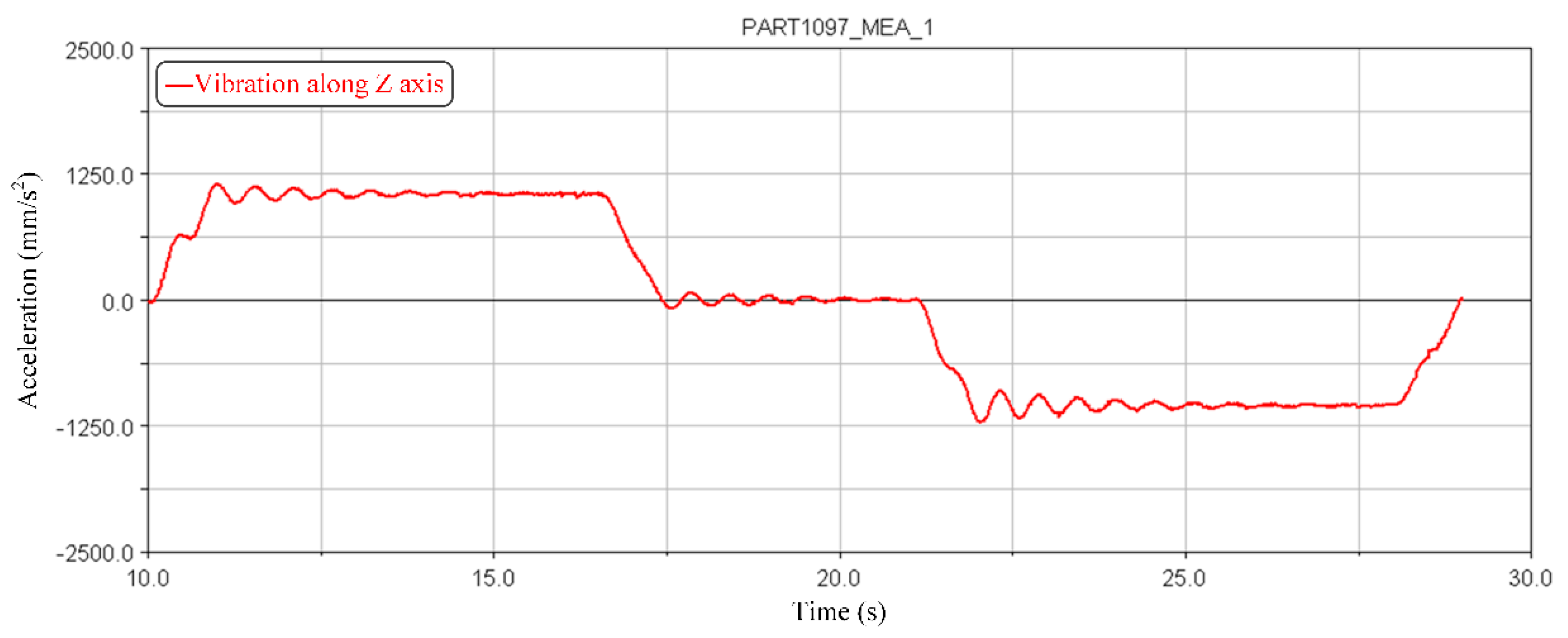
The key step of computing the PPIM lies in the natural of the exponential functions:

$$e^{H\tau }={(e^{(H\tau )/m})}^m$$

(55)

Assume $m=2^N$ and $N=20$. $\mathsf{\Delta }t=\tau /m$ is a minor temporal interval, in which Equations (56) and (57) are satisfied:

$$e^{H\Delta t}\approx I+H\Delta t+{(H\Delta t)}^2/2=I+T_a$$

(56)

$$T_a=H\Delta t(I+(H\Delta t)/2)$$

(57)

The scale of $T_a$ is so small that a precision loss would be encountered because of computer storing roundoff if being added with the unit matrix. Therefore, $T_a$ obtained from Equation (57) rather than $T_a+I$ could be stored in the computing device. Reserved terms in Equations (56) and (57) are determined by the computational precision requirement.

Equation (55) is decomposed to obtain the $T$ matrix:

$$T={\left[T_a+I\right]}^{2^N}={\left[T_a+I\right]}^{2^{N-1}}{\left[T_a+I\right]}^{2^{N-1}}$$

(58)

Because $(I+T_b)(I+T_c)=I+T_b+T_c+T_b{T}_c$, Equation (58) could be treated as a loop: $\mathrm{for}(iter=0; iter<N; iter++): T_a=2T_a+T_a{T}_a$. After the loop terminates, Equation (59) is implemented to obtain the PPIM:

$$T=I+T_a$$

(59)

5. Case Study

A case study is presented in this section taking the KLK2 high-speed elevator as an example, which is analyzed to constructed the EVM for simulation and computation. A comparison is then conducted between the obtained results and experimental data for elaboration and verification.

5.1. Operating Parameters of the Example Elevator

There are six steel traction ropes in KLK2 high-speed elevation system. The linear density of the steel ropes is $\rho =0.575 \mathrm{kg}/{\mathrm{m}}^2$, and the elastic modulus is $E=8\times {10}^{10} \mathrm{N}/{\mathrm{m}}^2$. The nominal diameter of the traction rope and tension rope is $d=13 \mathrm{mm}$. The tensile strength is $EA=4.72\times {10}^6 \mathrm{N}$, and the bending strength is $EI=22.16 \mathrm{N}·{\mathrm{m}}^2$. Mass of the lift car is $m_e=1250 \mathrm{kg}$. The pre-tension load is $F=750 \mathrm{N}$. The stiffness coefficient of pre-tension device $k_t=2\times {10}^3\mathrm{N}/\mathrm{m}$. The damping coefficient is $c_t=25 \mathrm{N}·\mathrm{s}/\mathrm{m}$. Length of the lift well is $l=225 \mathrm{m}$, and the lifting travel is $L=200 \mathrm{m}$. Nominal operating time from the bottom level to the top level is $t_{total}=30 \mathrm{s}$. Maximum operating speed and acceleration is $v_{max}=10 \mathrm{m}/\mathrm{s}$ and $a_{max}=1 \mathrm{m}/{\mathrm{s}}^2$. Take $g=9.81\mathrm{m}/{\mathrm{s}}^2$.

5.2. Operating State Equation of the Example Elevator

There are basically seven phases between the activation and termination according to the variations of lifting speed and acceleration, as shown in

Table 1. Seven phases of high-speed elevation operation state.

Phase	Time Used	Description
1	$t_1-t_0$	Acceleration increases to $a_e=-a_{max}>0$
2	$t_2-t_1$	Acceleration remains constant.
3	$t_3-t_2$	Acceleration reduces to $a_e=0$. Velocity increases to $v_e=-v_{max}>0$.
4	$t_4-t_3$	Velocity remains constant.
5	$t_5-t_4$	Deacceleration decreases to $a_e=a_{max}<0$
6	$t_6-t_5$	Deacceleration remains constant.
7	$t_6-t_7$	Deacceleration increases to $a_e=0$. Velocity increases to $v_e=0$.

. The activation time is recorded as $t_0$, and the end time of the $i$-th phase is denoted as $t_i$. The length, velocity, acceleration and jerk are represented as $l(t_i)$, $v_e(t_i)$, $a_e(t_i)$ and $j_e(t_i)$.

Change of jerk during acceleration phases shows a quadratic parabolic property. Because jerk is the third derivative of elevation, length of the traction rope could be represented as a quintic polynomial, which could be represented as:

$$l_e{}^{(i)}(t)=C_0^{(i)}+C_1^{(i)}(t-t_{i-1})+C_2^{(i)}{(t-t_{i-1})}^2+C_3^{(i)}{(t-t_{i-1})}^3+C_4^{(i)}{(t-t_{i-1})}^4+C_5^{(i)}{(t-t_{i-1})}^5.$$

(60)

Velocity, acceleration and jerk could be represented as the first, second and third derivatives of $l_e^{(i)}(t)$ in Equation (60):

$$\{\begin{array}{c}{a}_e{}^{(i)}(t)=2C_2^{(i)}+6C_3^{(i)}{(t-t_{i-1})}^1+12C_4^{(i)}{(t-t_{i-1})}^2+20C_5^{(i)}{(t-t_{i-1})}^3\\ j_e{}^{(i)}(t)=6C_3^{(i)}+24C_4^{(i)}{(t-t_{i-1})}^1+60C_5^{(i)}{(t-t_{i-1})}^2\\ v_e{}^{(i)}(t)=C_1^{(i)}+2C_2^{(i)}{(t-t_{i-1})}^1+3C_3^{(i)}{(t-t_{i-1})}^2+4C_4^{(i)}{(t-t_{i-1})}^3+5C_5^{(i)}{(t-t_{i-1})}^4\end{array}$$

(61)

where $t_{i-1}\le t\le t_i$, $t\in \left[1,7\right]$. $C_n^{(i)}(n=0,1,\dots ,5)$ are undetermined coefficients.

Jerk in phase 1 could be described by $j(t)=\alpha (t-t_0)+\beta {(t-t_0)}^2$. $\beta =-\alpha /(t_1-t_0)$ because the jerk is zero at time $t_1$. Assume the maximum acceleration is $a_{max}$, the maximum velocity is $v_{max}$, the initial length of the traction rope is $l(0)$, the elevation height is H, and the total operating time is $t_{total}$. Operation state equation of all these seven phases could be presented:

$$\{\begin{array}{c}{l}^{\left(1\right)}\left(t\right)=l\left(0\right)+\frac{\alpha {(t-t_0)}^4}{24}-\frac{\alpha {(t-t_0)}^5}{60t_j}\hfill \\ l^{\left(2\right)}\left(t\right)=l\left(t_1\right)+v\left(t_1\right)\left(t-t_1\right)+\frac{a\left(t_1\right)}{2}{(t-t_1)}^2\hfill \\ l^{\left(3\right)}\left(t\right)=l\left(t_2\right)+v\left(t_2\right)\left(t-t_2\right)+\frac{a\left(t_2\right)}{2}{(t-t_2)}^2-\frac{\alpha }{24}{(t-t_2)}^4+\frac{\alpha }{60t_j}{(t-t_2)}^5\hfill \\ l^{\left(4\right)}\left(t\right)=l\left(t_3\right)+v_{max}\left(t-t_3\right)\hfill \\ l^{\left(5\right)}\left(t\right)=l\left(t_4\right)+v\left(t_4\right)\left(t-t_4\right)-\frac{\alpha }{24}{(t-t_4)}^4+\frac{\alpha }{60t_j}{(t-t_4)}^5\hfill \\ l^{\left(6\right)}\left(t\right)=l\left(t_5\right)+v\left(t_5\right)\left(t-t_5\right)+\frac{a\left(t_5\right)}{2}{(t-t_5)}^2\hfill \\ l^{\left(7\right)}\left(t\right)=l\left(t_6\right)+v\left(t_6\right)\left(t-t_6\right)+\frac{a\left(t_6\right)}{2}{(t-t_6)}^2+\frac{\alpha }{24}{(t-t_6)}^4-\frac{\alpha }{60t_j}{(t-t_6)}^5\hfill \end{array}$$

(62)

where $a=(6a_{max}^3{v}_{max}^2)/{(t_{total}{v}_{max}{a}_{max}-a_{max}{l}_{total}-v_{max}^2)}^2$, and $t_j=\sqrt{(6a_{max})/\alpha }$.

5.3. EVM of KLK2 High-Speed Elevator

Substitute these parameters and operating state equations to Equations (28) and (29), and EVM of KLK2 high-speed elevator is obtained. Properties and types of EVM between phases are similar. EVM equations and boundary conditions of the first phase are listed in Equations (63)–(66) as an example:

$$\{\begin{array}{c}0.575\left(u_{tt}+2v{u}_{xt}+\left(0.074t^3-0.33t^2\right)u_x+v^2{u}_{xx}+\left(0.074t^3-0.33t^2\right)\right)-4.72\times {10}^6\left(u_{xx}+v_{1x}{v}_{xx}\right)\\ -\left[24500+5.635\left(225+0.0037t^5-0.027t^4-x\right)\right]-5.635\hfill \\ =4.72\times {10}^6\left(v_{2x}{v}_{1.xx}+v_{1.x}{v}_{2xx}+v_{2.x}{v}_{2.xx}\right),0<x<225+0.0037t^5-0.027t^4\hfill \\ 0.575\left(u_{tt}+2v{u}_{xt}+\left(0.074t^3-0.33t^2\right)u_x+v^2{u}_{xx}+\left(0.074t^3-0.33t^2\right)\right)-4.72\times {10}^6\left(u_{xx}+v_{1.x}{v}_{xx}\right)\hfill \\ -\left[24500+5.635\left(200-x\right)\right]-5.635\hfill \\ =4.72\times {10}^6\left(v_{2x}{v}_{1.xx}+v_{1.x}{v}_{2.xx}+v_{2x}{v}_{2.xx}\right),225+0.0037t^5-0.027t^4<x<200\hfill \end{array}$$

(63)

$$\{\begin{array}{c}0.575\left(v_{1.t}+2v{v}_{1.xt}+\left(0.074t^3-0.33t^2\right)v_{1.x}+v^2{v}_{1.xx}\right)\hfill \\ +\left[24500+5.635\left(225+0.0037t^5-0.027t^4-x\right)\right]v_{1x}\hfill \\ -4.72\times {10}^6\left(u_x{v}_{1.x}+u_x{v}_{1.xx}+\frac{1}{2}{v}_{1.x}^2\right)+22.16v_{1.x0xx}\hfill \\ =-0.575(v_{2.tt}+2v{v}_{2.xt}+a{v}_{2.x}{v}^2{v}_{2.xx})\hfill \\ +4.72\times {10}^6(u_{xx}{v}_{2x}+3v_{1x}{v}_{1.xx}{v}_{2x}+3v_{1.x}{v}_{2x}{v}_{2.xx}+u_x{v}_{2xx})\hfill \\ +4.72\times {10}^6(\frac{3}{2}{v}_{1.xx}{v}_{2.x}^2+\frac{3}{2}{v}_{1.x}^2{v}_{2.xx}+\frac{3}{2}{v}_{2.x}^2{v}_{2.xx})\hfill \\ +[24500+5.635(225+0.0037t^2-0.027t^4-x\left)\right]v_{2.x}\hfill \\ +[24500+5.635(225+0.0037t^2-0.027t^4-x\left)\right]v_{2.xx}\hfill \\ -22.16v_{2\times 000},0<x<225+0.0037t^5-0.027t^4\hfill \\ 0.575(v_{1.t}+2v{v}_{1.xt}+(0.074t^3-0.33t^2)v_{1.x}+v^2{v}_{1.xx})+[24500+5.635(200-x\left)\right]v_{1.x}\hfill \\ -4.72\times {10}^6\left(u_x{v}_{1.x}+u_x{v}_{1.xx}+\frac{1}{2}{v}_{1.x}^2\right)+22.16v_{1.x0xx}\hfill \\ =-0.575(v_{2,t}+2v{v}_{2.xt}+(0.074t^3-0.33t^2)v_{2.x}+v^2{v}_{2.xx}\hfill \\ +4.72\times {10}^6(u_{xx}{v}_{2.x}+3v_{1.x}{v}_{1.xx}{v}_{2.x}+3v_{1x}{v}_{2x}{v}_{2xx}+u_x{v}_{2xx})\hfill \\ +4.72\times {10}^6(\frac{3}{2}{v}_{1.2x}{v}_{2x}^2+\frac{3}{2}{v}_{1.x}^2{v}_{2xx}\frac{3}{2}{v}_{2x}^2{v}_{2.xx})+[24500+5.635(200-x\left)\right]v_{2x}\hfill \\ +[24500+5.635(200-x\left)\right]v_{2xx}-22.16v_{2,x00x},225+0.0037t^5-0.027t^4<x<200\hfill \end{array}$$

(64)

$$\{\begin{array}{c}0.575\left(w_{1.t}+2v{w}_{1.xt}+\left(0.074t^3-0.33t^2\right)w_{1.x}+v^2{w}_{1.xx}\right)\hfill \\ +\left[24500+5.635\left(225+0.0037t^5-0.027t^4-x\right)\right]w_{1.x}\hfill \\ -4.72\times {10}^6\left(u_x{w}_{1.x}+u_x{w}_{1.xx}+\frac{1}{2}{w}_{1.x}^2\right)+22.16w_{1.x00x}\hfill \\ =-0.575(w_{2tt}+2v{w}_{2.xt}+(0.074t^3-0.33t^2)w_{2.x}{v}^2{w}_{2.xx}\hfill \\ +4.72\times {10}^6(u_{xx}{w}_{2x}+3w_{1.x}{w}_{1.xx}{w}_{2.x}+3w_{1.x}{w}_{2.x}{w}_{2.xx}+u_x{w}_{2.xx})\hfill \\ +4.72\times {10}^6(\frac{3}{2}{w}_{1.xx}{w}_{2.x}^2+\frac{3}{2}{w}_{1.x}^2{w}_{2.xx}+\frac{3}{2}{w}_{2.x}^2{w}_{2.xx})\hfill \\ +[24500+5.635(225+0.0037t^2-0.027t^4-x\left)\right]w_{2.x}\hfill \\ +[24500+5.635(225+0.0037t^2-0.027t^4-x\left)\right]w_{2.xx}\hfill \\ -22.16w_{2.x00x},0<x<225+0.0037t^5-0.027t^4\hfill \\ 0.575w(v_{1.t}+2v{w}_{2.xt}+(0.074t^3-0.33t^2)w_{1.x}+v^2{w}_{1.xx})+[24500+5.635(200-x\left)\right]w_{1.x}\hfill \\ -4.72\times {10}^6\left(u_x{w}_{1.x}+u_x{w}_{1.xx}+\frac{1}{2}{w}_{1.x}^2\right)+22.16w_{1.x0x}\hfill \\ =-0.575(w_{2tt}+2v{w}_{2.xt}+(0.074t^3-0.33t^2)w_{2x}+v^2{w}_{2.xx}\hfill \\ +4.72\times {10}^6(u_x{w}_{2x}+3v_{1.x}{w}_{1.xx}{w}_{2x}+3w_{1.x}{w}_{2.x}{w}_{2.xx}+u_x{w}_{2.xx})\hfill \\ +4.72\times {10}^6(\frac{3}{2}{w}_{1.xx}{w}_{2x}^2+\frac{3}{2}{w}_{1.x}^2{w}_{2.xx}\frac{3}{2}{w}_{2.x}^2{w}_{2.xx})+[24500+5.635(200-x\left)\right]w_{2.x}\hfill \\ +[24500+5.635(200-x\left)\right]w_{2,xx}-22.16w_{2,x0xx},225+0.0037t^5-0.027t^4<x<200\hfill \end{array}$$

(65)

$$\{\begin{array}{c}2500u_{tt}+2v{u}_{xx}+(0.074t^3-0.33t^2)u_x+v^2{u}_{xx}+(0.074t^3-0.33t^2)-5.635\hfill \\ {+[24500+5.635(225+0.0037t^5-0.027t^4-x\left)\right]+4.72\times {10}^6{u}_x+2.36\times {10}^6{v}^{2}x)}_{r^{-1}}\hfill \\ -[24500+5.635(200-x\left)\right]+ES{u}_x+\frac{1}{2}ES{v}_x^2=0,x=225+0.0037t^5-0.027t^4\hfill \\ [24500+5.635(200-x\left)\right]+4.72\times {10}^6(u_x+\frac{1}{2}{v}_x^2)+25(u_t+v{u}_x)+2\times {10}^{5}u=0,x=200\end{array}$$

(66)

5.4. Solution of the Established EVM

Use the solution method proposed in Section 4.2 and segment the traction rope to 10 parts. Therefore, initial displacements of the discrete nodes along Y and Z axis are $q_{v,j}(0)=0.1\sin (\pi (j-1)/n)$ and $q_{w,j}(0)=0.1\sin (\pi (j-1)/n)$ respectively, when $t=0$ and $1\le j\le n$. There are structural flexibility and remaining degrees of freedom because of loose joints in the fabrication and installation of the lift car, the guide rail, the guiding sheave and the traction rope. Therefore, after the simulation begins and before the elevation process is started, the lift car would initially tend to gain stability under the effect of self-gravity and free-hanging. The kinematic conditions would appear unstable for a short period of time before self-stability is reached. As the real starting point of time, the systematic response would be recorded 10 s after the simulation is started. The main reason of the 10-s gap is to leave some time for automatic balancing before valuable data could be produced and collected. To ensure the accuracy and reliability of experimental simulation and analysis, all those curves are recorded and presented after the 10-s gap. Take the time step as 0.01 s, and the vibrational acceleration at the joint point of the traction string and the lift car along X, Y, Z axis is obtained and presented in Figure 3, Figure 4 and Figure 5 respectively. Key indicators including $Max(P_k)/P_k$ and A95 could estimate the operating vibration [40]. As a result, $Max(P_k)/P_k$ along X, Y, Z axis are 0.376$\mathrm{m}/{\mathrm{s}}^2$, 0.317$\mathrm{m}/{\mathrm{s}}^2$, 0.503$\mathrm{m}/{\mathrm{s}}^2$ respectively. A95 are 0.251$\mathrm{m}/{\mathrm{s}}^2$, 0.118$\mathrm{m}/{\mathrm{s}}^2$, 0.429$\mathrm{m}/{\mathrm{s}}^2$ along X, Y, Z axis.

5.5. Comparison and Verification between Vibration Models

To verify the effectiveness and efficiency of the established EVM model, the DVM model [41] is built and simulated to obtain the response curve of vibrational acceleration at the joint point between the traction string and the lift car. As shown in Figure 6, Figure 7 and Figure 8, $Max(P_k)/P_k$ along X, Y, Z axis are 0.363$\mathrm{m}/{\mathrm{s}}^2$, 0.305$\mathrm{m}/{\mathrm{s}}^2$, 0.495$\mathrm{m}/{\mathrm{s}}^2$ respectively. A95, along X, Y, Z axis are 0.245$\mathrm{m}/{\mathrm{s}}^2$, 0.114$\mathrm{m}/{\mathrm{s}}^2$, 0.417$\mathrm{m}/{\mathrm{s}}^2$.

Prototype experiments and measurements for the KLK2 high-speed elevator are conducted in a 288-meter elevator experimental tower to obtain the vibration along X, Y, Z axis. The experimental devices are shown in Figure 9. Figure 9a shows the elevator experimental tower. Figure 9b shows the PMT EVA-625 elevator vibration analysis system of physical measurement technologies (PMT) [42]. The testing and measuring site is shown in Figure 9c.

Vibrational acceleration curve obtained from PMT EVA-625 is shown in Figure 10, in which the four curves from top to bottom are (I) variation curve of the absolute velocity during the height lifting process, (II) variation curve of the vibrational acceleration along X axis, (III) variation curve of the vibrational acceleration along Y axis, (IV) variation curve of the vibrational acceleration along Z axis. $Max(P_k)/P_k$ along X, Y, Z axis are 0.384$\mathrm{m}/{\mathrm{s}}^2$, 0.324$\mathrm{m}/{\mathrm{s}}^2$, 0.512$\mathrm{m}/{\mathrm{s}}^2$ respectively. A95, along X, Y, Z axis are 0.264 $\mathrm{m}/{\mathrm{s}}^2$, 0.120$\mathrm{m}/{\mathrm{s}}^2$, 0.440$\mathrm{m}/{\mathrm{s}}^2$.

A comparison between the obtained indicators through DVM method, prototype experiments, and the proposed EVM method is shown in

Table 2. A comparison of the obtained indicators through the DVM method, prototype experiments and the proposed EVM method.

		DVM Method $(m/s^2)$	EVM Method $(m/s^2)$	Prototype Experiments $(m/s^2)$
$Max(P_k)/P_k$	X axis	0.363	0.376	0.384
	Y axis	0.305	0.317	0.324
	Z axis	0.495	0.503	0.512
A95	X axis	0.245	0.251	0.264
	Y axis	0.114	0.118	0.120
	Z axis	0.417	0.429	0.440

. $Max(P_k)/P_k$ obtained from the DVM method are 0.363$\mathrm{m}/{\mathrm{s}}^2$, 0.305$\mathrm{m}/{\mathrm{s}}^2$, 0.495$\mathrm{m}/{\mathrm{s}}^2$ along X, Y, Z axis respectively, whose deviations from the experimental results are 5.47%, 5.86%, 3.32%. A95 are 0.245$\mathrm{m}/{\mathrm{s}}^2$, 0.114$\mathrm{m}/{\mathrm{s}}^2$, 0.417$\mathrm{m}/{\mathrm{s}}^2$ along X, Y, Z axis, whose deviations from the experimental results are 7.20%, 5.00%, 5.23% respectively. As a contrary, $Max(P_k)/P_k$ obtained from the proposed EVM method are 0.376$\mathrm{m}/{\mathrm{s}}^2$, 0.317$\mathrm{m}/{\mathrm{s}}^2$, 0.503$\mathrm{m}/{\mathrm{s}}^2$ along X, Y, Z axis, whose deviations from the experimental results are 2.08%, 2.16%, 1.76%. A95 are 0.251$\mathrm{m}/{\mathrm{s}}^2$, 0.118$\mathrm{m}/{\mathrm{s}}^2$, 0.429$\mathrm{m}/{\mathrm{s}}^2$, whose deviations from the experimental results are 4.92%, 1.67% and 2.50% respectively. Obviously, the proposed EVM method could achieve more precise results than the conventional DVM method. It is worth noting that the deviations from experimental data are less than 5%. The manufacturing, fabrication, installation error and the operating environment would significantly enhance systematic vibration. However, as detailed in Section 3.3, these influencing factors are not carefully considered when establishing EVM. The proposed EVM would probably appear more accurate and the simulation results would be closer to the experimental data when precision engineering and periodic inspection could relieve their impacts. Therefore, the example study has shown the efficiency, potential and reliability of the proposed EVM method.

6. Conclusions

An EVM method is proposed in this paper to describe the multi-direction coupling vibration properties of high-speed traction system, which would further benefit vibration control and optimization design. The main contributions are:

• The characteristics of the traction system is analyzed and simulated using masses, springs and dampers. A combination of kinematic energy, elastic potential energy and virtual work provides a description of the multi-direction coupling vibration properties, based on which EVM method is established.
• EVM contains a complicated partial differential equation set with unlimited degrees of freedom and time-varying parameters. This paper discretizes the EVM to an ordinary differential equation set through the time-varying element method, and obtain the solutions using the Gaussian precise integration method.
• An example study is conducted using KLK2 high-speed elevator. EVM is then established to obtain the simulation results and the solutions of vibrational acceleration indices, $Max(P_k)/P_k$ and A95, along X, Y, Z axis. The obtained results are then compared with the conventional DVM method and experimental data of KLK2 prototype. The proposed EVM method could achieve more accurate results than the conventional DVM method, and deviations of these indicators are less than 5%. In this way, efficiency, potential and reliability of the proposed EVM method have been elaborated and verified.

References

1. Fung, R.F.; Lin, J.H.; Yao, C.M. Vibration analysis and suppression control of an elevator string actuated by a PM synchronous servo motor. J. Sound Vib. 1997, 206, 399–423. [Google Scholar] [CrossRef]
2. Peng, Q.; Jiang, A.; Yuan, H.; Huang, G.; He, S.; Li, S. Study on Theoretical Model and Test Method of Vertical Vibration of Elevator Traction System. Math. Probl. Eng. 2020, 2020. [Google Scholar] [CrossRef] [Green Version]
3. Crespo, R.S.; Kaczmarczyk, S.; Picton, P.; Su, H. Modelling and simulation of a stationary high-rise elevator system to predict the dynamic interactions between its components. Int. J. Mech. Sci. 2018, 137, 24–45. [Google Scholar] [CrossRef]
4. Kaczmarczyk, S.; Andrew, J.P.; Adams, J.P. The Modelling and Prediction of the Influence of Building Vibration on the Dynamic Response of Elevator Ropes. Mater. Sci. Forum 2003, 440–441, 489–496. [Google Scholar] [CrossRef]
5. Yang, D.H.; Kim, K.Y.; Kwak, M.K.; Lee, S. Dynamic modeling and experiments on the coupled vibrations of building and elevator ropes. J. Sound Vib. 2017, 390, 164–191. [Google Scholar] [CrossRef]
6. Kobayashi, S.; Yoshimura, T.; Noguchi, N.; Omiya, A. Estimation of dynamic characteristics of an elevator car using operational modal analysis. Nihon Kikai Gakkai Ronbunshu C Hen/Trans. Jpn. Soc. Mech. Eng. Part C 2008, 74, 548–553. [Google Scholar] [CrossRef] [Green Version]
7. Zhang, R.; Wang, C.; Zhang, Q. Response analysis of the composite random vibration of a high-speed elevator considering the nonlinearity of guide shoe. J. Braz. Soc. Mech. Sci. Eng. 2018, 40. [Google Scholar] [CrossRef]
8. Zhang, R.; Wang, C.; Zhang, Q.; Liu, J. Response analysis of non-linear compound random vibration of a high-speed elevator. J. Mech. Sci. Technol. 2019, 33, 51–63. [Google Scholar] [CrossRef]
9. Wee, H.; Kim, Y.Y.; Jung, H.; Lee, G.N. Nonlinear rate-dependent stick-slip phenomena: Modeling and parameter estimation. Int. J. Solids Struct. 2001, 38, 1415–1431. [Google Scholar] [CrossRef]
10. Yang, Z.; Zhang, Q.; Zhang, R.; Zhang, L. Transverse Vibration Response of a Super High-Speed Elevator under Air Disturbance. Int. J. Struct. Stab. Dyn. 2019, 19, 1950103. [Google Scholar] [CrossRef]
11. Taplak, H.; Erkaya, S.; Yildirim, Ş.; Uzmay, I. The Use of Neural Network Predictors for Analyzing the Elevator Vibrations. Arab. J. Sci. Eng. 2014, 39, 1157–1170. [Google Scholar] [CrossRef]
12. Utsunomiya, K.; Okamoto, K.I.; Yumura, T.; Funai, K.; Kuraoka, H. Active roller guide system for high-speed elevators. Elev. World 2002, 50, 198–205. [Google Scholar]
13. Mirabdollah Yani, R.; Ghodsi, R.; Darabi, E. A closed-form solution for nonlinear oscillation and stability analyses of the elevator cable in a drum drive elevator system experiencing free vibration. Commun. Nonlinear Sci. Numer. Simul. 2012, 17, 4467–4484. [Google Scholar] [CrossRef]
14. Teshima, N.; Kamimura, K.; Nagai, M.; Kou, S.; Kamada, T. Vibration Control of Ultra High Speed Elevator by Active Mass Damper: 1st Report, Study by Optimal Control Theory. Nihon Kikai Gakkai Ronbunshu, C Hen/Trans. Jpn. Soc. Mech. Eng. Part C 1999, 65, 3479–3485. [Google Scholar] [CrossRef]
15. Gaiko, N.V.; van Horssen, W.T. Resonances and vibrations in an elevator cable system due to boundary sway. J. Sound Vib. 2018, 424, 272–292. [Google Scholar] [CrossRef]
16. Otsuki, M.; Ushijima, Y.; Yoshida, K.; Kimura, H.; Nakagawa, T. Application of nonstationary sliding mode control to suppression of transverse vibration of elevator rope using input device with gaps. JSME Int. J. Ser. C Mech. Syst. Mach. Elem. Manuf. 2006, 49, 385–394. [Google Scholar] [CrossRef] [Green Version]
17. Yamazaki, Y.; Tomisawa, M.; Okada, K.; Sugiyama, Y. Vibration control of super-high-speed elevators: (Car vibration control method based on computer simulation and experiment using a full-size car model). JSME Int. J. Ser. C Dyn. Control Robot. Des. Manuf. 1997, 40, 74–81. [Google Scholar] [CrossRef]
18. Kimura, H.; Nakagawa, T. Vibration analysis of elevator rope with vibration suppressor. Nihon Kikai Gakkai Ronbunshu C Hen/Trans. Jpn. Soc. Mech. Eng. Part C 2005, 71, 442–447. [Google Scholar] [CrossRef]
19. Arrasate, X.; Kaczmarczyk, S.; Almandoz, G.; Abete, J.M.; Isasa, I. The modelling, simulation and experimental testing of the dynamic responses of an elevator system. Mech. Syst. Signal Process. 2014, 42, 258–282. [Google Scholar] [CrossRef]
20. Santo, D.R.; Balthazar, J.M.; Tusset, A.M.; Piccirilo, V.; Brasil, R.M.L.R.F.; Silveira, M. On nonlinear horizontal dynamics and vibrations control for high-speed elevators. JVC J. Vib. Control 2018, 24, 825–838. [Google Scholar] [CrossRef]
21. Nakano, K.; Hayashi, R.; Suda, Y.; Noguchi, N.; Arakawa, A. Active Vibration Control of an Elevator Car Using Two Rotary Actuators. J. Syst. Des. Dyn. 2011, 5, 155–163. [Google Scholar] [CrossRef]
22. Noguchi, N.; Arakawa, A.; Miyoshi, K.; Kawamura, Y.; Yoshimura, T. Active vibration control technology for elevator cars considering controllability. Nihon Kikai Gakkai Ronbunshu C Hen/Trans. Jpn. Soc. Mech. Eng. Part C 2013, 79, 3192–3205. [Google Scholar] [CrossRef] [Green Version]
23. Noguchi, N.; Arakawa, A.; Miyata, K.; Yoshimura, T.; Shin, S. Study on Active Vibration Control for High-Speed Elevators. J. Syst. Des. Dyn. 2011, 5, 164–179. [Google Scholar] [CrossRef]
24. Utsunomiya, K.; Okamoto, K.; Yumura, T.; Sakuma, Y. Vibration control of high-speed elevators taking account of electricity consumption reduction. Nihon Kikai Gakkai Ronbunshu C Hen/Trans. Jpn. Soc. Mech. Eng. Part C 2006, 72, 2048–2055. [Google Scholar] [CrossRef]
25. Utsunomiya, K. Vibration Damping Device for an Elevator. J. Acoust. Soc. Am. 2011, 129, 3419. [Google Scholar] [CrossRef]
26. Baek, K.-H.; Kim, K.-Y.; Kwak, M.-K. Dynamic Modeling and Controller Design for Active Control of High-speed Elevator Front-back Vibrations. Trans. Korean Soc. Noise Vib. Eng. 2011, 21, 74–80. [Google Scholar] [CrossRef] [Green Version]
27. Kim, D.Y.; Park, M.R.; Sim, J.H.; Hong, J.P. Advanced Method of Selecting Number of Poles and Slots for Low-Frequency Vibration Reduction of Traction Motor for Elevator. IEEE/ASME Trans. Mechatron. 2017, 22, 1554–1562. [Google Scholar] [CrossRef]
28. Kang, J.K.; Sul, S.K. Vertical-vibration control of elevator using estimated car acceleration feedback compensation. IEEE Trans. Ind. Electron. 2000, 47, 91–99. [Google Scholar] [CrossRef]
29. Nguyen, T.X.; Miura, N.; Sone, A. Analysis and control of vibration of ropes in a high-rise elevator under earthquake excitation. Earthq. Eng. Eng. Vib. 2019, 18, 447–460. [Google Scholar] [CrossRef]
30. Dos Santos, L.C.C.; Brasil, R.M.L.R.F.; Balthazar, J.M.; Piccirillo, V.; Tusset, A.M.; Santo, D.R. Active vibration control of an elevator system using magnetorheological damper actuator. Int. J. Nonlinear Dyn. Control 2017, 1, 114. [Google Scholar] [CrossRef]
31. Fan, W.; Zhu, W.D. Dynamic analysis of an elevator traveling cable using a singularity-free beam formulation. In Proceedings of the ASME Design Engineering Technical Conference, Cleveland, OH, USA, 6–9 August 2017; Volume 6. [Google Scholar]
32. Rijanto, E.; Muramatsu, T.; Tagawa, Y. Control of elevator having parametric vibration using LPV control method: Simulation study in the case of constant vertical velocity. In Proceedings of the IEEE Conference on Control Applications, Kohala Coast, HI, USA, 22–27 August 1999. [Google Scholar]
33. Mutoh, N.; Kagomiya, K.; Kurosawa, T.; Konya, M.; Andoh, T. Horizontal Vibration Suppression Method Suitable for Super-High-Speed Elevators. IEEJ Trans. Ind. Appl. 1998, 118, 353–362. [Google Scholar] [CrossRef] [Green Version]
34. Feng, Y.; Zhang, J.; Zhao, Y. Modeling and robust control of horizontal vibrations for high-speed elevator. JVC/J. Vib. Control 2009, 15, 1375–1396. [Google Scholar] [CrossRef]
35. Zhang, P.; Bao, J.H.; Zhu, C.M. Dynamic analysis of hoisting viscous damping string with time-varying length. J. Phys. Conf. Ser. 2013, 448. [Google Scholar] [CrossRef]
36. Kimura, H.; Ito, H.; Fujita, Y.; Nakagawa, T. Forced vibration analysis of an elevator rope with both ends moving. J. Vib. Acoust. Trans. ASME 2007, 129, 471–477. [Google Scholar] [CrossRef]
37. Lu, Y. Dynamics of the Flexble Multibody Syestems; Higher Education Press: Beijing, China, 1996. [Google Scholar]
38. Irgens, F. Continuum Mechanics; Springer: Berlin/Heidelberg, Germany, 2008; ISBN 978-3-540-74298-2. [Google Scholar]
39. Wan-Xie, Z. On precise integration method. J. Comput. Appl. Math. 2004. [Google Scholar] [CrossRef] [Green Version]
40. ISO 18738-1:2012, Lifts (Elevators)-Measurement of Ride Quality[S]. 2012. Available online: https://www.iso.org/standard/54395.html (accessed on 7 July 2020).
41. Shabana, A.A. Dynamics of Multibody Systems, 2nd ed.; Cambridge University Press: Cambridge, UK, 1998; ISBN 13: 978-0521594462. [Google Scholar]
42. The World’s Standard of Measurement Elevator Ride Quality, Vibration & Sound. Available online: https://www.pmtvib.com/eva-625 (accessed on 7 July 2020).
Figure 1. Basic structure of a high-speed traction system.
Energies 13 04821 g001
Figure 2. Multi-direction vibration characteristic of the high-speed traction system.
Energies 13 04821 g002
Figure 3. Vibrational acceleration response along X axis using EVM.
Energies 13 04821 g003
Figure 4. Vibrational acceleration response along Y axis using EVM.
Energies 13 04821 g004
Figure 5. Vibrational acceleration response along Z axis using EVM.
Energies 13 04821 g005
Figure 6. Vibrational acceleration response along X axis using DVM.
Energies 13 04821 g006
Figure 7. Vibrational acceleration response along Y axis using DVM.
Energies 13 04821 g007
Figure 8. Vibrational acceleration response along Z axis using DVM.
Energies 13 04821 g008
Figure 9. Prototype experiments and measurements for the KLK2 high-speed elevator.
Energies 13 04821 g009
Figure 10. Curves of lifting velocity and vibrational acceleration obtained from PMT EVA-625.
Energies 13 04821 g010