Analysis of V-Gutter Reacting Flow Dynamics Using Proper Orthogonal and Dynamic Mode Decompositions

Abstract

The current work is focused on investigating the potential of data-driven post-processing techniques, including proper orthogonal decomposition (POD) and dynamic mode decomposition (DMD) for flame dynamics. Large-eddy simulation (LES) of a V-gutter premixed flame was performed with two Reynolds numbers. The flame transfer function (FTF) was calculated. The POD and DMD were used for the analysis of the flame structures, wake shedding frequency, etc. The results acquired by different methods were also compared. The FTF results indicate that the flames have proportional, inertial, and delay components. The POD method could capture the shedding wake motion and shear layer motion. The excited DMD modes corresponded to the shear layer flames’ swing and convect motions in certain directions. Both POD and DMD could help to identify the wake shedding frequency. However, this large-scale flame oscillation is not presented in the FTF results. The negative growth rates of the decomposed mode confirm that the shear layer stabilized flame was more stable than the flame possessing a wake instability. The corresponding combustor design could be guided by the above results.

1. Introduction

Lean premixed combustion is of interest due to the fact that it has been widely used in modern gas turbine combustors to control nitrogen oxides (NOx) emission. However, the consequent thermoacoustic issue also comes up. The thermoacoustic issue is expressed as the pressure fluctuating inside the combustor. When the dry low NOx (DLN) combustion system in the FT8 engine was first developed, the frequency of the dynamic pressure fluctuation showed a 200–400 Hz range [1]. This pulsation has been damped by adding additional acoustic resonators [2] while more complicated designs should be considered, such as the cooling of resonators. The thermoacoustic issue is caused by a combination of the heat release rate (HRR) and the pressure fluctuation. Such unsteady heat release is one of the manifestations for flame dynamics. The analysis road map is based on Rayleigh criteria [3]. If the phase between the pressure fluctuation and the heat release rate (HRR) fluctuation is less than π/4, and the integral of their product’s volume is larger than the damping of the system, the thermoacoustic issue occurs [4]. The factors that influence the flame dynamics can be categorized as burner aerodynamics, combustor acoustics, and coherent structures of fluid [5]. The coherent structures inside the combustor are critical to flame dynamics. Nevertheless, the analysis of coherent structures is normally limited in fluid dynamics and flow field. Therefore, it is interesting to further research the relationships between coherent structures and natural gas premixed flame dynamics.

To analyze the flame dynamics, one of the traditional methods is modeling the flame response to acoustical perturbations as a linear time-invariant (LTI) system. The flame transfer function (FTF), which is the heat release rate (HRR) response in the frequency domain, is used to obtain the frequency domain information. The FTF can be derived by analytical [6,7], Computational fluid dynamics (CFD) [8], and experimental approaches [9,10,11]. An identification scheme employing a Wiener filter was proposed [12], which can use a single large-eddy simulation (LES) to determine the flame response. This method has been already used in the FTF calculations for axial swirlers [13] and conical swirlers in industrial burners [14,15], and the numerical results have been demonstrated to be in agreement with the experimental results [16]. Nevertheless, more efforts should made to open the black box of the FTF in order to understand the root cause of the HRR’s high gain.

The widely accepted proper orthogonal decomposition (POD) method has been used for understanding the relationship between the FTF and multi-fluid structures. This method decomposes the combustion field into a few principal components based on the variance maximization theory. Researchers observed periodic fluctuations in the reaction zone and obtained the dominant frequency by POD [17]. In addition, swirling flames have been analyzed as the correlation between the POD modes and reprehensive fields [14,15,16,17,18]. The POD remedies the deficiency of the pattern in the FTF. Even similar POD modes make different contributions to the FTF results. The POD-FTF technique is applied to examine a vortex breakdown of the stabilized flame in the related study [19]. In their work, the fluctuations were split into different sources to explain the FTF results. However, two aspects limit the utilization of POD in flame dynamics analysis. One aspect is that the mode, which triggers thermoacoustic issues, might not be the one with the highest energy content. Owing to this phenomenon, the lower energy content modes might be neglected or treated as artificial modes in the POD analysis. The other issue is that the usage of the POD method is normally limited to the understanding of the periodic stable condition.

Therefore, dynamic mode decomposition (DMD) was proposed [20,21]. The DMD results provide the growth rate and the corresponding amplitude spectrum. In addition, DMD can be used to determine the corresponding frequency. This post-processing method has been used for the FTF calculation [22], flame dynamics examination, and limits the cycle prediction [23]. The POD and DMD techniques are used to analyze the results from flame imaging and correctly extract the dominant fluctuations [24], which are related to the fundamental oscillation frequency.

Whether the relationships between coherent structures and flame dynamics can be figured out by the above data-driven methods is worth considering in detail. A simple premixed flame called the V-gutter flame was investigated for this purpose. The V-gutter flame holder is used in a variety of propulsion systems for stabilizing flames [25,26]. As described by many researchers, the shear layer is generated at the edge of the V-gutter flame holder [27,28]. The burned mixture flows into a recirculation zone, which acts as a torch to facilitate the ignition inside the radical pool. A related study shows that a bluff body stabilized flow field contains Kelvin Helmholtz (KH) and Bérnard von Karman (BVK) instabilities when the Reynolds number is less than 200,000 [29]. The KH instability is generated by the shear layer and symmetrically distributed on each side beyond the edge of the bluff body. By contrast, the BVK instability exhibits a large-scale vortex roll-up and periodical shedding at the end of the recirculation zone. When the flame is generated, the vorticity produced by the exothermicity interacts with the two abovementioned instabilities. The wake shedding (BVK instability) can be suppressed via large flow dilatation, e.g., $T_b/T_u$, in which $T_b$ represents the burnt temperature, and $T_u$ represents the unburnt mixture temperature. However, in cases with low $T_b/T_u$, a sinuous wake might still be present [30], which affects the flame.

Although many operating conditions lead to the above instabilities [31,32], the most important factor is the flow structures generated by the V-gutters themselves. Compared to the swirling flame, the V-gutter flame has clearer low-order flow structures, which can show the potential of the POD and DMD methods.

In this work, the V-gutter premixed flame was modeled by LES. Datasets with two inflow conditions (different inflow Reynolds numbers) were generated. Two instable flame structures were reproduced by regulating the Reynolds number. The corresponding FTFs were extracted. The POD and DMD methods were employed to separate the turbulent flames into detailed mode shapes. The growth rates were calculated to identify which modes were more unstable while the frequency band for each mode was compared with the FTF results. Thus, the flame dynamics, the mode shapes, and the frequency bands, were linked together. The relationship between the FTF frequency and flow/flame structure was further analyzed via the above results.

2. Algorithm for Post-Processing Methods

2.1. POD Algorithm

The snapshots method proposed in a related study [33] was used for both POD and DMD. The snapshots were collected during the LES procedure. Only the flame field is evaluated inside the data matrix. The raw data matrix $X_0^{ }$ represents the evolution of the heat release rate. $X_{std}^{ }$ is the data matrix after the standardization of $X_0^{ }$. The calculation uses the singular vector decomposition (SVD). It should be mentioned that the number of principal components ($k$) is selected according to the cumulative variance of the principal components, which should exceed the predefined level (80%) or exist as a clear inflection point in the scree plot. The time coefficient of each POD mode was calculated using the principal component and snapshots.

2.2. DMD Algorithm

In the DMD technique, the previously mentioned raw data matrix $X_0^{ }$ is separated into two matrixes, $X,\left(\mathrm{t}=0,1,\dots ,\mathrm{n}-1\right)$ and $X\text{’},\left(\mathrm{t}=1,\dots ,\mathrm{n}\right)$ with a single time step difference. The operator $A$, which represents the short-term dynamic system evolution, can be written as $X^{\prime }=AX$. The operator can be calculated as $A=X\text{’}{X}^{+}$, in which $X^{+}$ is the pseudo-inverse of $X$. To reduce the computational cost due to the large size of A [21], the DMD algorithm uses the single value decomposition (SVD) procedure $X=U\Sigma V^{*}$. and keeps the first fifty modes because the first several modes might not have high fluctuations. By projecting $A$ onto the left eigenvector $U$ by using $U^{*}AU$, the low-rank operator $\tilde{A}$ can be calculated as $\tilde{A}=U^{*}X\text{’}V{\Sigma }^{+}$. The eigenvalue of $A$ is the eigenvalue $\Lambda$ of $\tilde{A}$ and eigenvector $w^i$ of matrix $\tilde{A}$, as $\tilde{A}W=W\Lambda$. The corresponding spectra of the $i$-th eigenvalue are determined as $f=Im\left(log{\lambda }_i\right)/\left(2\pi \ast dt\right)$, where $Im$ is the imaginary part, and $dt$ is the constant interval between snapshots. The real part $\left(Re\right)$ of the eigenvalue is used to compute the temporal growth rate as $a=Re\left(log{\lambda }_i\right)/\left(2\pi \ast dt\right)$. The global stability of the system can be estimated by the sign of the growth rate. A positive value indicates the growth of the instability, a zero value indicates a pure oscillating behavior, and a negative value indicates that the mode is decaying. This procedure yields a pair of frequencies with opposite signs. However, for the same absolute value of frequency, only one growth rate value exists. Finally, the eigenvector $\Phi$ of $A$ is computed as $\Phi =X\text{’}V{\Sigma }^{-1}W$.

2.3. FTF Procedure

The steady premixed methane–air flame can be assumed as a linear time-invariant system (LTI) under low excitation [34]. The flame response is assumed as a unit impulse response (HRR fluctuations at the flame front) to a series of inlet impulses (perturbations before the flame). In this work, the incompressible condition with a perfect premixed inlet boundary is implemented. Therefore, the coherent structure impact on the flame dynamics can be isolated from the chamber acoustics. The FTF can be defined as

$$FT{F}_u=\frac{\dot{Q\text{’}}/\overline{\dot{Q}}}{u\text{’}/\overline{u}}.$$

(1)

Here, $\left({·}^{\prime }\right)$ represents the instantaneous value subtracted by the average value, $\left(\overline{·}\right)$ represents the ensembled average value, and the heat release rate $\dot{Q}$ is calculated as the volume integral of the product formation rate (PFR) over the simulation domain. The procedure is determined by considering the relation between the cross-correlation of the numerator and denominator and the autocorrelation of the denominator. This equation has been proved and is named as the Wiener–Hopf equation [35]. The current paper also employs sampling with a replacement to avoid the lack of samples due to the short time of the LES.

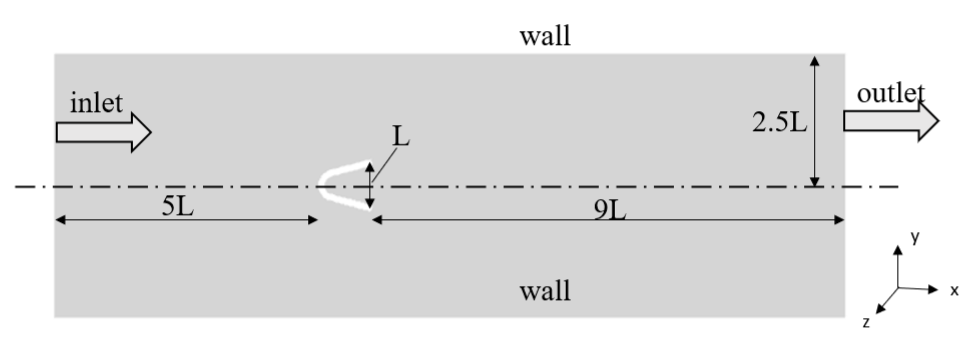
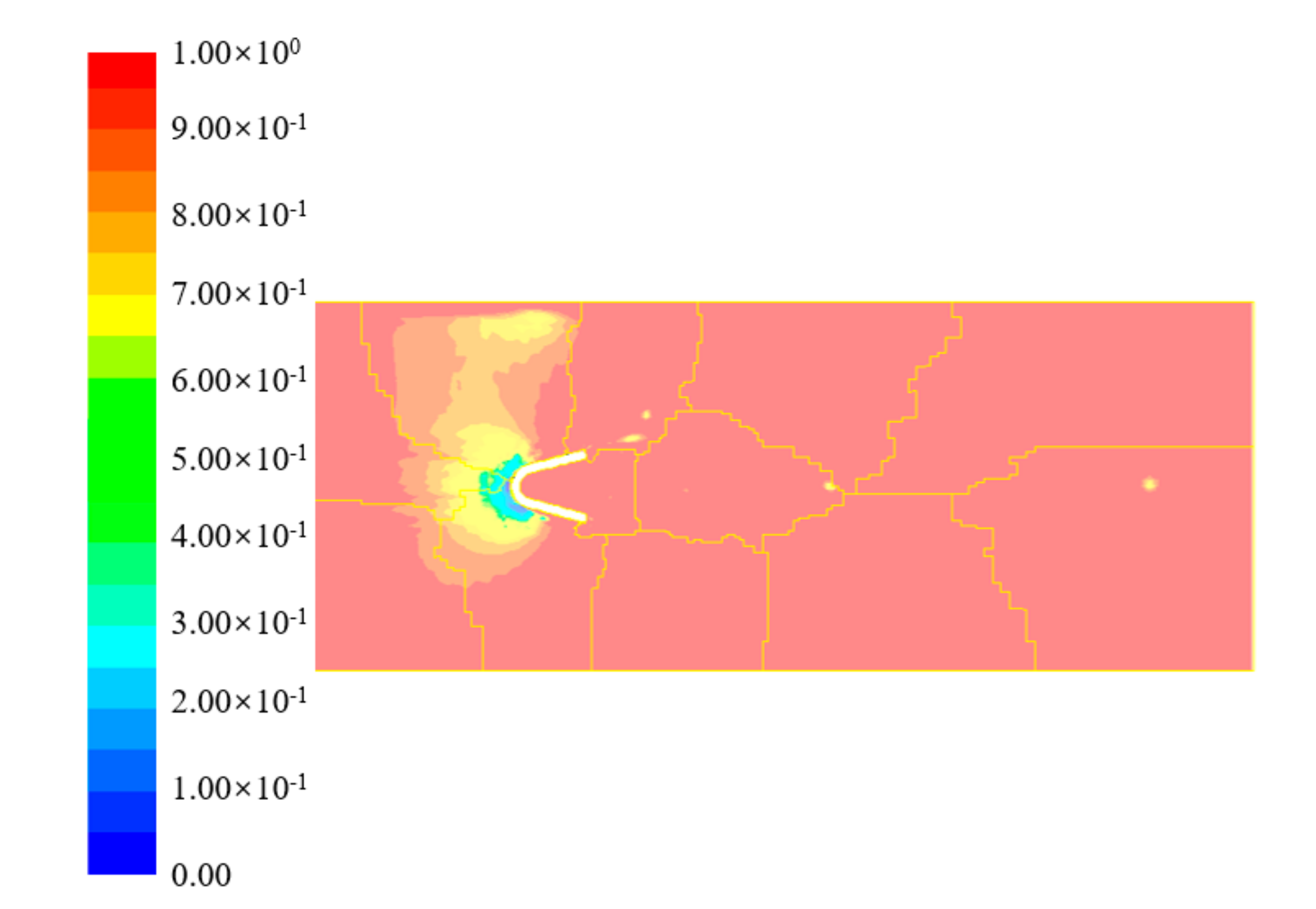
3. V-Gutter Geometry and the Numerical Method

To limit the research to investigate only the flame dynamics induced by the vortex field, the CFD domain is simplified as no fuel injector geometry is presented. The inlet methane–air mixture includes perfectly premixed methane and air. Therefore, the flame dynamics analysis does not involve the examination of the mixing quality. The V-gutter flame holder works in a confined flow field (Figure 1). This aspect constrains the flame front to not follow the opening angle ($\beta$) of the V-gutter flame holder.

As shown in Figure 1, the V-gutter has a width L = 20 mm at the open side, which is considered as the characteristic length. The wall thickness of the V-gutter is 1/8th the value of L. The inlet is located 5 L from the leading edge of the V-gutter, and the outlet is located 9 L from the trailing edge of the V-gutter. The simulation domain is symmetrical with 2.5 L from the center line on each side. The domain is a 1/5 L thin layer, with a symmetric boundary set in the CFD.

The mesh is drawn using with legacy software Gambit. The pave type mesh is applied near the V-gutter region, and the remaining domain is filled with a hexa-mesh. The same meshes are later used for the LES analysis, albeit with a refined shear layer and a recirculation zone to meet the requirements of the 85% energy index [36]. The pave-type mesh resolution near the trailing edge of the V-gutter flame holder is 0.25 mm per cell side. In the shear layer region, the hexa-type mesh resolution is 0.67 mm per cell side. In the recirculation zone, the mesh resolution is 1 mm in the y-direction and 0.7 mm in the x-direction. The upper and lower boundaries are set as a no-slip adiabatic wall.

There is no mesh independent for the LES mesh, especially for implicit LES. Historically, the mesh quality for LES was a hot topic in 1990–2010. For implicit LES, as Pope proposed the energy index [37] methods, the grid quality uses the idea to count resolved Turbulent kinetic energy (TKE) over the overall TKE. Then, grid quality using single-grid estimators [36,38,39,40] was developed, and the power spectrum method [41] and the correlation method [42] were proposed. By using multiple meshes, numerical errors can be separated from modeling errors [39]. Estimators with three-grid LESs were also released [43].

So far, only the one-grid estimator remains well reported on the academic side due to its simplicity. This work uses this idea.

The Celik-defined energy-based index is

$$M=\frac{k_{res}}{k_{tot}}=\frac{k_{res}}{k_{res}+k_{sgs}}.$$

(2)

Here, k represents the kinetic energy. res—resolved, sgs—SGS modeled. The calculated index based on the LES mesh is below:

The index contour is shown in Figure 2.

The simulations were performed under atmospheric conditions, with a premixed gas, including air and methane, at a temperature of 591 K. GRI-Mech 3.0 [44] (53 species, 325 reactions) was used to generate the reaction table. The tabulation was performed considering the adiabatic energy treatment and chemical equilibrium conditions. When initiating LES, the wall-adapting local eddy viscosity (WALE) model was employed for the subgrid-scale (SGS) model. The bounded central differencing (BCD) scheme was applied for spatial discretization. The second-order implicit scheme was applied for the transient formulation, and the time step size was ${10}^{-5}$ s.

Partially premixed turbulent combustion was modeled using the Zimont turbulent flame speed closure (TFC) model [45,46], which assumes that the vortices are smaller than the flame thickness that can penetrate the flame zone, and later thicken and wrinkle the flame fronts. The flame front is identified by solving the transport equation of the progress variable (PV). The source term in the PV transport equation is closed by the turbulent flame speed. Since the purpose of this work is to explore the use of data-driven methods to display the modes for a certain frequency, the boundaries cause flame burnt near the lean blowoff, and the flame stretch effect is not considered. In the TFC model, the product formation rate (PFR) indicates the main heat release region and is used in the FTF analysis.

Three LESs were performed for each selected condition: the first LES was to generate the turbulent structures and stabilize the flame. The second LES was to record the snapshots for the POD and DMD analysis. The final LES, which takes 0.2 s, was used for the DMD and FTF data acquisition. The velocity excitation was applied in the final stage LES. The discrete random binary signal (DRBS) was recommended [12]. This method has already been applied to calculate the FTF for the swirl flame [34] and industrial combustors [47]. Figure 3 shows the excitation signal with an amplitude of 10%. Figure 3b indicates that no short-term linear autocorrelation exists in the signal.

The LESs were realized using ANSYS Fluent 18.2 and an AMD EPYC Rome CPU from the CST Cloud in China. The pre- and post-processing were performed using Python 3.6.

In order to validate the precision of the current LES setup using the bluff body stabilized premixed flame, corresponding LES simulations were performed in this work. The LES result was compared with experimental data and Reynolds-averaged Navier-Stokes equations (RANS) data. Axial average velocity profiles and the average temperature profiles from the experimental data, the Reynolds stress mode (RSM) model, the k-ε model, and the LES results are depicted in Figure 4 and Figure 5, respectively. It can be found that axial velocity profiles calculated by LES can match the experimental data better than those from the RSM or k-ε model. With respect to the mean temperature profiles, the discrepancy in the central temperature is minor between the LES results and the experimental ones. The temperature curves near the sides can also track the original values effectively.

4. Results

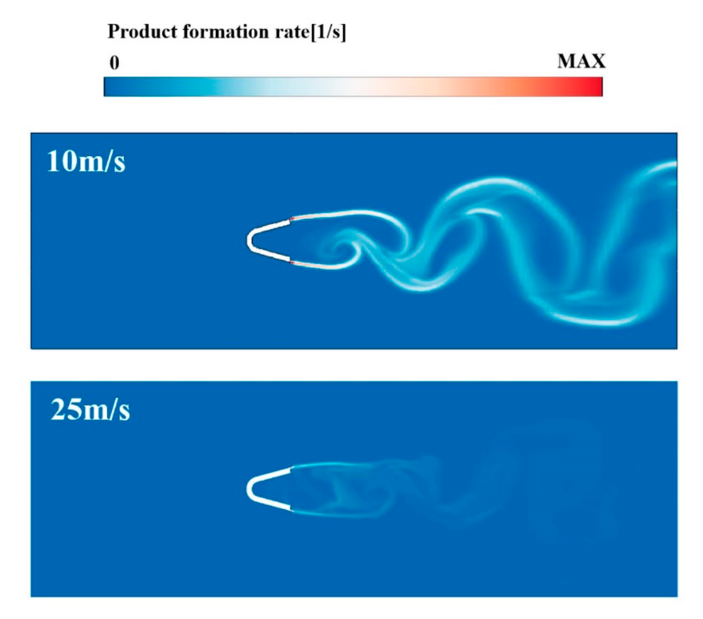
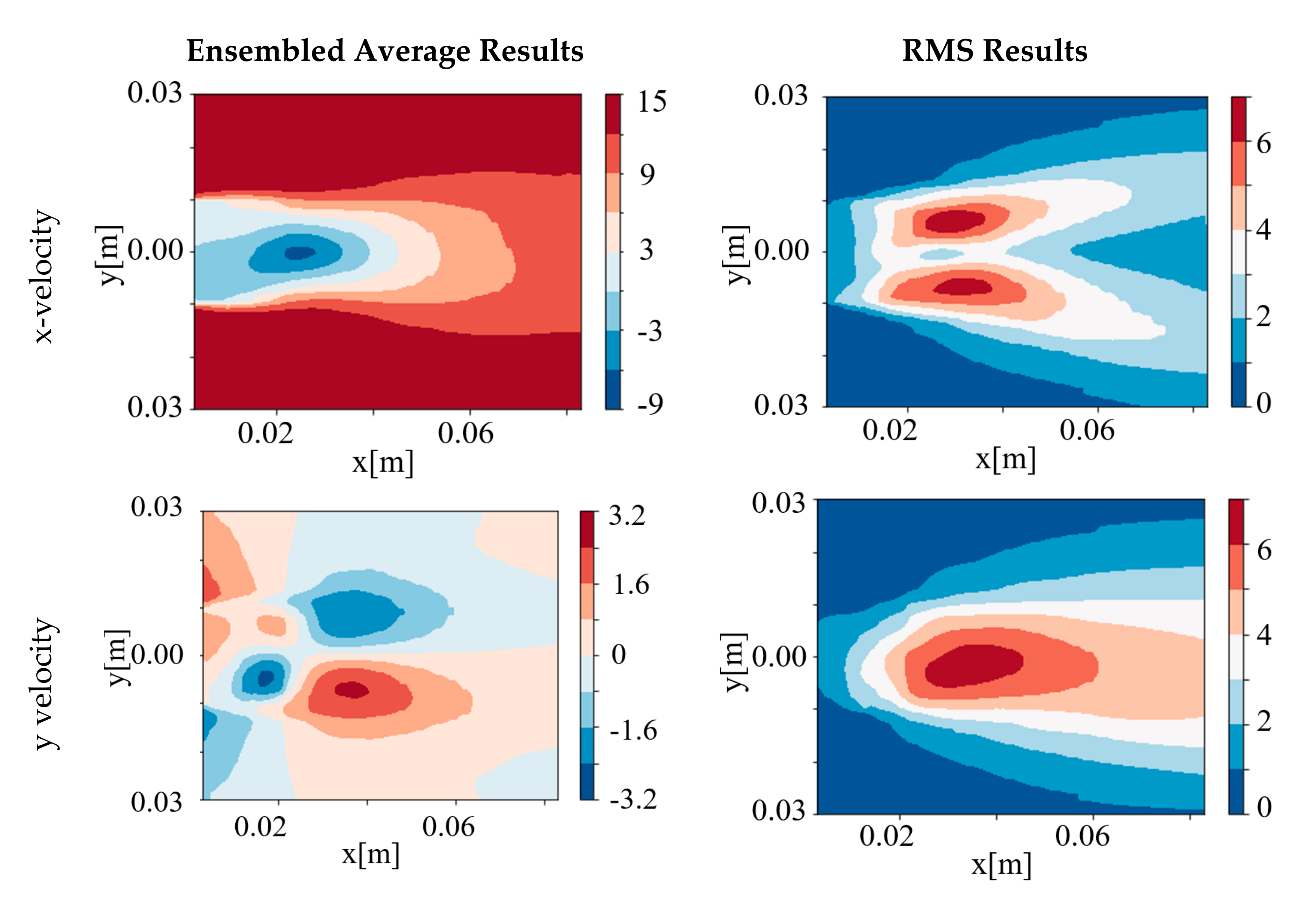
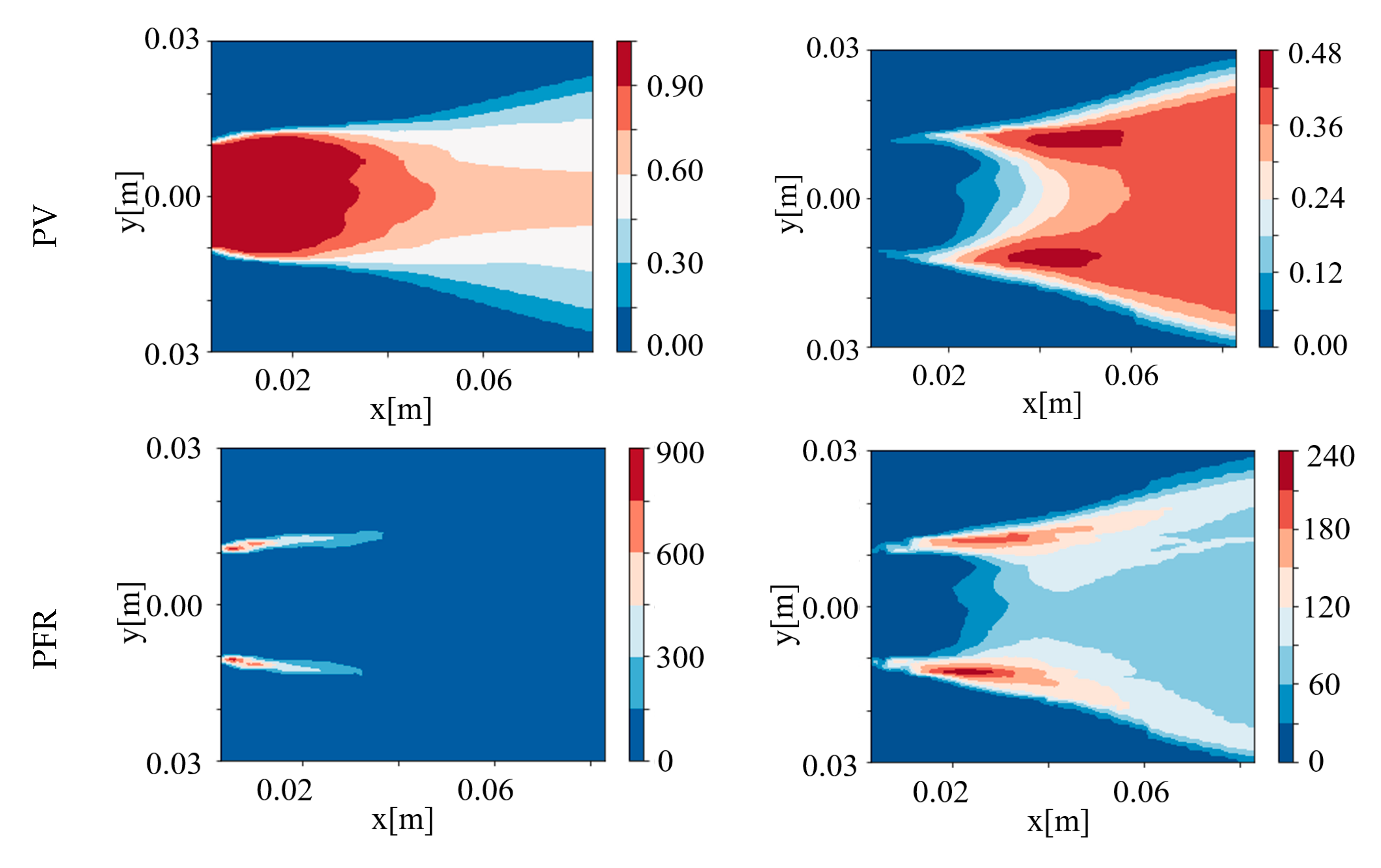
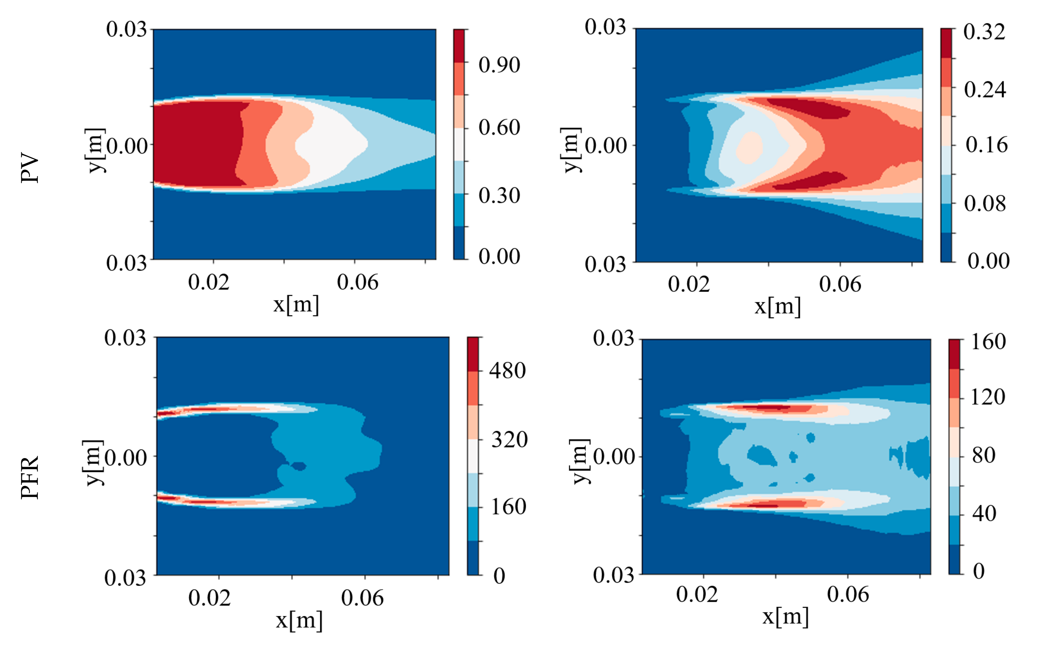
4.1. Instantaneous and Averaged Results

According to relevant research, ($V/W)(1/P{T}^{1.5})=f\left(\varphi \right)$), except for the operating condition (pressure P and inflow temperature T), the inflow velocity ($U$), equivalence ratio ($\varphi$), and V-gutter width ($W$) are the three major parameters that influence the stability of the V-gutter flame. Steady RANS has been performed in a two-level full factorial design of experiment (DoE) way for eight cases. The residence time and the mean x-velocity are used to estimate the continuously burning trend. The RANS results show that (1) the residence time decreases with an increase in the inflow velocity and opening angle; however, it increases slightly with an increase of 20% in the equivalence ratio. (2) The mean x-velocity in the recirculation zone increases with an increase in the equivalence ratio but it decreases with increases in the opening angle and inflow velocity. Finally, the parameters are chosen, as in

Table 1. Boundary conditions for LES.

	V-Gutter Opening Angle $\mathit{\beta }$ ($°$)	Inflow Velocity U (m/s)	Equivalence Ratio ($\mathit{\varphi }$)
Condition 1	30	10	0.5148
Condition 2	30	25	0. 5148

. In condition 1, the Reynolds number is 6898, and in condition 2, the Reynolds number is 17,244.

In Figure 6, the instantaneous results indicate that in condition 1, the flame burning in the shear layer is more stable; however, it suffers from wake shedding. The KH instability and BVK instability are present. The flame in condition 2 burns in the shear layers and the recirculation zones covered by the shear layers. Even though the Reynolds numbers in both conditions are less than 200,000, the BVK instability presents in the case with smaller Reynolds numbers.

The instantaneous fields are used to determine the observation window size, which is 4.25 L right after the V-gutter edge and +/− 1.5 L in the y-direction. The spatial resolution of the observation window is 1 mm/grid size, which is coarser than the mesh. The snapshots are exported every 25 time steps. Each snapshot contains velocity components and the flame components (PFR and PV). In this study, 1024 snapshots are collected for each condition. The ensembled average results and the corresponding Root Mean Square (RMS) for condition 1 are presented in Figure 7, which shows that the recirculation region is 1–2 L downstream of the V-gutter. The high fluctuating y-velocity lies in the recirculation region. The PV is concentrated inside the Recirculation zone (RZ), while the highly fluctuating PV is located outside RZ on both sides of the shear layer region. The PFR demonstrates the high heat release region beginning at the trailing edge of the V-gutter. The shape of the RMS PFR indicates that the flame fluctuates outwards in the shear layer region.

Figure 8 shows the ensembled average and RMS results for condition 2. The general difference between conditions 1 and 2 lies in the shape of the recirculation zone. The mean and RMS x-velocity patterns reduce 1.5 L downstream of the V-gutter in condition 2. The recirculation region is split into upstream and downstream parts. Both parts show a low level of x-velocity fluctuations. The PV and PFR show that the flame is confined in the area surrounded by the shear layer.

To summarize the above findings, the averaged y-direction velocity indicates that the fluids flow outwards away from the centerline at the end of the recirculation zone in both conditions, which indicates a potential shedding wake in both conditions. Downstream of RZ, there is fluid flow towards the centerline due to the confined domain. This inwards flow covers the outwards flow in condition 2. Meanwhile, the x-direction velocity field in condition 2 shows the recirculation zone is approximately 20 mm longer than condition 1. Both reasons led to the BVK instability in condition 2 being smaller than that in condition 1. Although both PV and PFR can represent the flame field, the PFR yields a better representation of the flame front. The PFR is employed in the following analysis. Although the large-scale shedding motion can be explained by the above analysis, the frequency cannot be obtained from the mean and RMS field. Without the information in the frequency domain, it is difficult to estimate the flame dynamics. Therefore, the POD and DMD methods are introduced.

4.2. POD Results

The first five modes are kept for the two-condition POD analysis due to the reason that there are clear inflation points in the scree plots.

The first five POD modes in the two conditions are compared in Figure 9. In condition 1, the most fluctuations in the PFR value occurred at the shear layer and extends outwards (spectrum not shown here, approximately 150 Hz). The location and mode shape indicate this was induced by KH instability. The 3rd–4th modes (approximately 300 Hz) exhibit a high fluctuating PFR value, which is symmetrical and located downstream of the stable recirculation zone between the shear layer flame, which is the shedding wake motion induced by BVK instability. The link between these BVK and KH motions is the fluid itself. Part of the shear layer fluid flowed into the recirculation zone. When the fluid was transported downstream and leaves the recirculation zone (1st–2nd POD modes), it was captured by the counter-rotating vortices in the shedding wake motion (3rd–4th POD modes). The PFR contour of the 5th mode (rang 420–470 Hz) exhibits a slightly asymmetric mode shape, which is more like the combination of the shear layer motion and the shedding wake motion.

In condition 2, the 1st mode corresponds to the high fluctuating flame region, which is the shear layer region. The corresponding spectrum (not shown here) was extremely gradual. The 2nd and 3rd modes (approximately 400 Hz) represent that the flame fronts in these two modes are asymmetrical to the centerline. Compared to condition 1, this motion indicates the shear layer flame, which is with the KH instability. The fluctuating motion is downstream of the recirculation zone. The 4th mode has a shape similar to that of mode 1, and it corresponds to extremely slow motion. The 5th mode (approximately 800 Hz) represents large-scale shedding wake, which is with the BVK instability. The location is still after the stable recirculation zone. Due to these two reasons, (1) the BVK mode is not spreading in the y-direction nor the x-direction like the 3rd and 4th POD modes in condition 1 and (2) the BVK’s eigenvalue is the fifth in the order. Thus, the shedding wake motion is not so obvious in condition 2. The frequency of the 5th mode is approximately double of the 3rd and 4th modes; this finding is similar to condition 1.

The Lissajous plots, which are mainly used to show the phase difference between modes, are shown in Figure 10 for the condition 1 results. Scatters of the first two modes lie in a ring inside the unit circle. These findings indicate that the time coefficients have a similar amplitude and frequency, albeit with a 90° phase shift. As shown by the scatter plot of the time coefficients of the 1st and 4th modes (Figure 10b), the 4th mode has one-half the amplitude, two times the dominant frequency, and a 45° phase shift compared to mode 1. The 3rd and 4th modes are in pair with a 90° phase shift. Considering the results of the time coefficients, modes, and phase relations from the Lissajous plot, it is possible to conclude that the 1st–2nd and 3rd–4th modes are in pairs.

The frequency of the BVK instability can be calculated as $f=St·\frac{u}{D}$, which is the universal Strouhal number $St=0.28$ [29]. The V-gutter opening length is selected as the characteristic length $D=L=0.02\mathrm{m}$. If the inflow velocity $U=10\mathrm{m}/\mathrm{s}$ is selected, the calculated shedding vortex frequency is approximately 140 Hz. The most similar frequency in the POD results is 150 Hz. However, the modes’ shape indicates that it is the shear layer motion. Instead, the 3rd and 4th modes, which are approximately 300 Hz, represent the large-scale wake motion. Hence, the POD provides a different BVK frequency, as estimated in the literature.

The Lissajous plots for condition 2 are shown in Figure 11. Results indicate that the amplitudes of 2nd-3rd modes are the same with values less than 1 with a phase shift of 90°. The amplitude of the 4th mode is 80% of the 2nd mode with a phase shift of 45°. The amplitude of the 5th mode is 80% of the 2nd mode with a phase shift of 90°.

Compared to the condition 1 results, both the wake motion and shear layer motion appear in condition 2 as well. Though the wake mode occurs, this motion is not spreading in the x- or y-direction like in condition 1.

4.3. DMD and FTF Results

4.3.1. Flame Dynamics and Dynamic Mode in Condition 1

Figure 12 presents the FTF result for condition 1 in the form of a Bode plot. Up to 80 Hz, a positive gain occurs. The gain trend indicates an inertial element (−20 dB slope) and a proportional component exists. The phase trend indicates that a time lag component is present. The results of simple curve fitting are represented by the red line. The time lag is approximately 0.8 ms. If the time lag is calculated based on transport in the x-direction, and the corresponding fluctuating structure is of the order of 8 mm. This value is calculated using the averaged x-velocity, which is 10 m/s set at the inlet boundary. If the time lag is calculated based on the transport in the y-direction and the averaged y-velocity at the flame region is approximately 3 m/s, as shown in Figure 7, then the corresponding length is 2.4 mm. The first two POD modes in Figure 9 predicted the fluctuating shear layer flame fronts in the y-direction to be less than 5 mm, while the 3rd and 4th POD modes, which contain multiple structures, are in the wake region. Hence, it is difficult to link the POD modes with the FTF by directly viewing the frequency and mode shapes. The POD results cannot predict if the first two modes are excited modes or not, nor the stability trend of these two modes. In order to better understand the FTF results and flame stability, DMD was performed.

Since the FTF calculation uses only the heat release rate (PFR), the data matrix used in the DMD procedure will only contain the PFR values. Firstly, it should be mentioned that the DMD results exhibit a slightly different spectrum if excitation occurs. As shown in Figure 13a, the solid black dot (and lines) are with excitation. When excitation is present, the lower spectrum (<100 Hz) exhibits increased growth rate and frequency values even though the growth rate values are negative. For a higher spectrum, the frequency and growth rate levels remain almost the same. Figure 13b shows the distribution of the first 50 eigenvalues relative to the unit circle. To explain the FTF results, only the excited DMD modes are presented in the following part.

The selected modes are summarized in

Table 2. DMD modes selected from condition 1 with excitation.

POD		DMD
Mode Number	Frequency [Hz]	Mode Number	Frequency [Hz]	Growth Rate [1/s]
No corresponding modes in the first five POD modes		43	23	−22
		45	60	−12
1	150	35	152	−3
2		39	141	−8
3	300	27	307	−9
4
5	420–470	17	460	−10
		19	429	−11
No corresponding modes in the first five POD modes		11	594	−13

. The 43rd and 45th modes are selected because these two modes have frequency bands less than 80 Hz, which corresponds to a higher FTF gain. Therefore, the coherence between the flame response to perturbations and the shape is linked. It should be noted that this correlation is not causal. It only shows that the fluctuating flame structures influenced by the inlet excitation are the shear layer flame fluctuating in the y-direction. The remaining modes are selected due to their higher growth rate values. Figure 14 presents the real part of these DMD modes.

To compare these modes with the POD modes, both the mode numbers and frequency bands of the POD and DMD modes are summarized, as follows.

As shown in Figure 14.

(1)

The higher growth rate DMD modes.

Except the 43rd and 45th DMD modes, the resulting DMD modes are found to be symmetric to the centerline. This indicates the fluctuating shear layer flame is swung up and down around each branch of the shear layer region. This fluctuating flame is not showing in the first ten modes in the unexcited POD result.

(2)

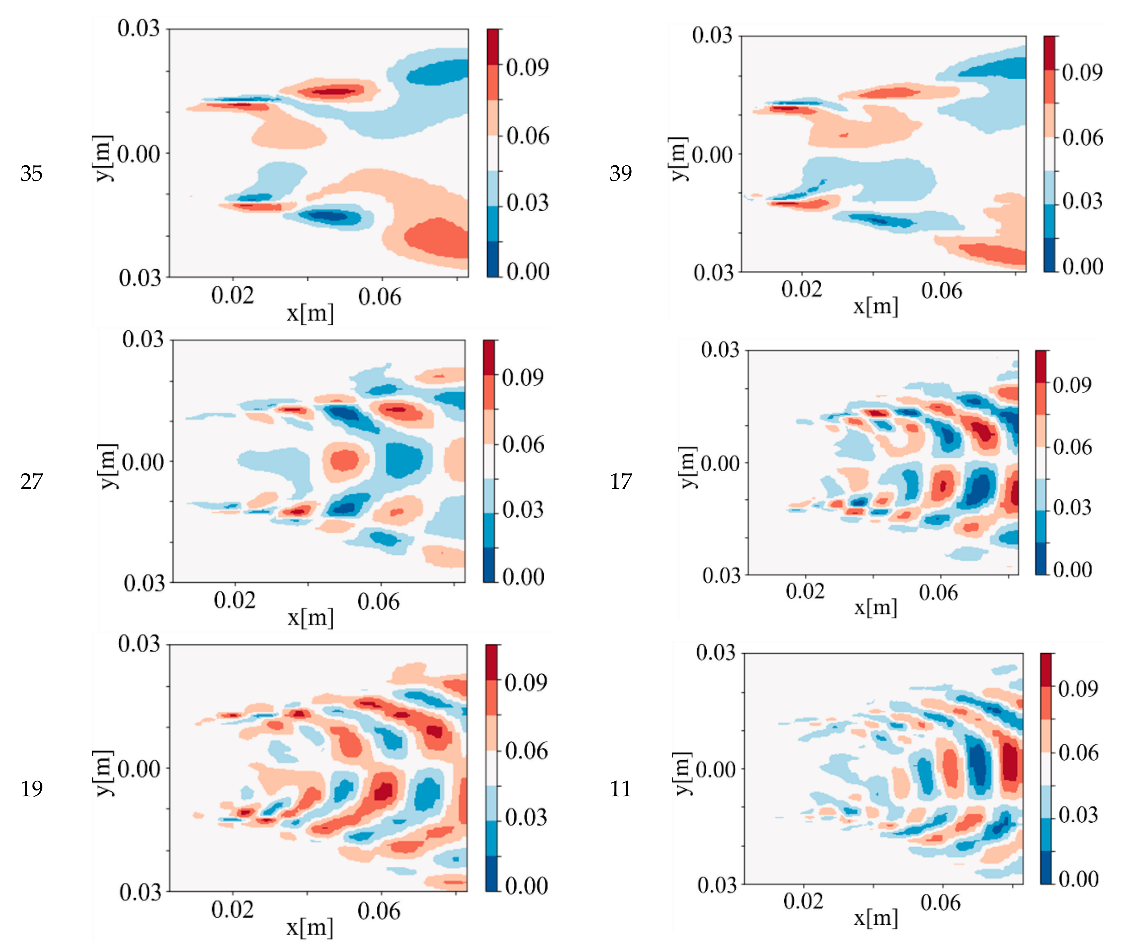
The 35th and 39th DMD modes.

Both modes have a frequency close to 140 Hz, which is close to the BVK instability. However, like the analysis in the POD section, these asymmetric modes represent the shear layer flame with KH instability. It is noted that the shapes of the 35th and 39th modes are the same, not the 90$°$ phase shift like the POD modes in a pair.

(3)

The 27th, 17th, and 19th DMD modes.

They can be found in agreement with the POD results.

(4)

The 11th DMD mode is the second order of the 27th DMD mode.

Although the POD modes are arranged based on their eigenvalue, which is calculated as a higher covariance value of the correlation coefficient matrix, POD modes are identical to the DMD modes (Table 2), even though the selection of the DMD modes is based on a higher growth rate.

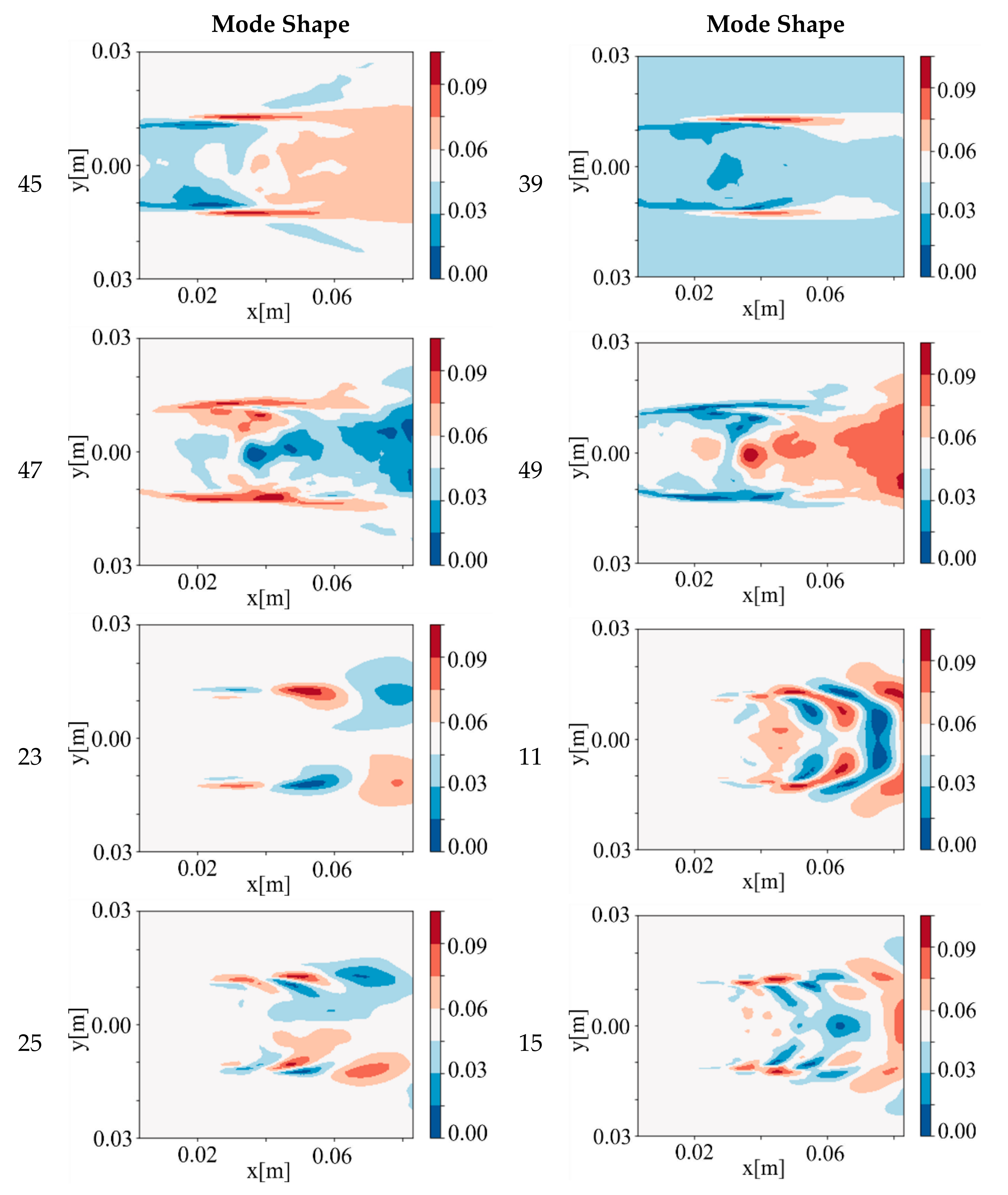
4.3.2. Flame Dynamics and Dynamic Mode in Condition 2

In Figure 15, the FTF result indicates that the flame in condition 2 is excited in the frequency bands lower than 120 Hz. The red line is the curve fitting, which indicates that the FTF has an inertial element, proportional component, and time lag. The time lag is estimated as 0.4 ms, which corresponds to 10 mm in the x-direction or 0.4–2.4 mm in the y-direction, based on the averaged velocity component (Figure 8).

Figure 16 shows the shift in the spectrum due to the inlet excitation. Up to 120 Hz, the frequency bands are shifted to a higher value. For a frequency larger than 120 Hz, the modes, which have higher growth rates, are not strongly influenced by excitation. The eigenvalues in the two conditions are printed with a unit circle in Figure 16b. This scatter indicates that the flame in condition 2 is more susceptible than that in condition 1 (Figure 13b).

Table 3. Spectrum and growth rate of the DMD.

POD		DMD
Mode Number	Frequency [Hz]	Mode Number	Frequency [Hz]	Growth Rate [1/s]
No corresponding modes in the first five POD modes		45	42	−65
		39	92	−83
		47	21	−194
		49	30	−139
2, 3	400	23	383	−11
No corresponding modes in the first five POD modes		25	394	−39
5	800	11	782	−32
		15	778	−68

presents the spectrum and growth rate of the DMD modes. The similar modes in the POD are listed on the left. The 45th, 39th, 47th, and 49th DMD modes have a frequency band lower than 120 Hz. To analyze the DMD modes, Figure 17 presents the mode shapes.

(1)

The 47th and 49th DMD modes.

Only the 47th and 49th modes are strongly influenced by the excitation. The frequency of these modes increased from less than 20 Hz to more than 20 Hz. In addition, those two modes occur in pairs to represent the fluctuating behavior between the stable recirculation zone and the wake. Those modes are not shown in the POD results. Although the 1st and 4th POD modes also exhibit extremely low-frequency bands, they indicate that the flame fluctuates locate at the shear layer near the end of the recirculation zone.

(2)

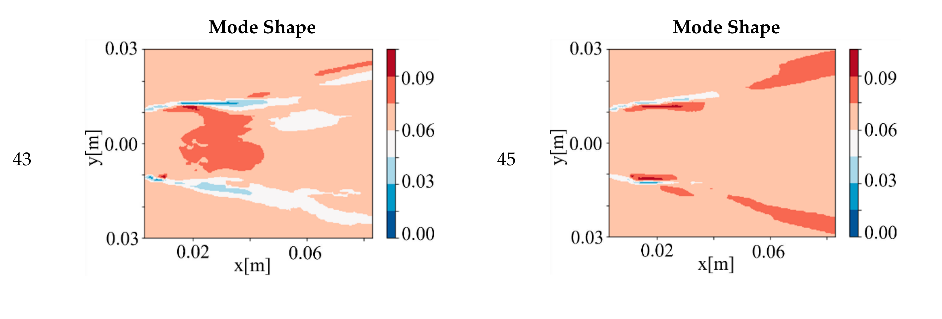
The 45th and 39th DMD modes.

Those two modes indicate the fluctuating shear layer flame fronts swing around each branch of the shear layer and convect downstream. This thin layer corresponds to the time delay calculated length scale (0.4–2.4 mm).

(3)

The 23rd–25th DMD modes.

These two modes are asymmetric, which indicates the shear layer flame forms due to the KH instability. The difference between the 45th–39th mode pair and 23rd–25th mode pair is the rotating direction. The 23rd mode corresponds to the 2nd–3rd POD modes. In the meantime, the 23rd DMD mode has the highest growth rates, which means the fluctuation in the y-direction is the strongest motion in this flame.

(4)

The 11th and 15th DMD modes.

They exhibit a similar structure and frequency band like those of the 5th POD mode.

Comparing the results between the POD and DMD, it can be noted that some POD modes in condition 1 can be found in the DMD results. However, in condition 2, the 1st and 4th POD mode cannot be found in the DMD results. This can be explained by the POD algorithm, which tends to not guarantee that different structures are separated, but only the data size is reduced by selecting the first several modes based on the variance. Therefore, the POD mode, which is a linear combination of the elements in the covariance matrix, might not represent a single flow/flame structure and thus has only a single frequency. Nevertheless, there is a single flame structure with its single frequency that is distinguished by the DMD. It was also observed that the first several POD modes might exhibit different shapes and frequencies compared to those pertaining to the DMD results.

Comparing the DMD results between conditions 1 and 2, they indicate that for DMD modes in condition 2, the growth rate level is generally lower than that in condition 1. Thus, the flame in condition 2 shows a more stable trend than that in condition 1.

5. Conclusions

In this work, stabilization of a premixed methane flame by a V-gutter flame holder has been performed with two inflow Reynolds number using LES. The results indicate that the condition with a lower Reynolds number would lead to a higher chance of presenting wake instability. The FTFs for two flames are released for the first time. In order to understand the flame structures corresponding to the frequency bands, the two data-driven post-processing methods POD and DMD are used, and the results are compared. The three post-processing methods deepen our understanding of different aspects as follows:

(1)

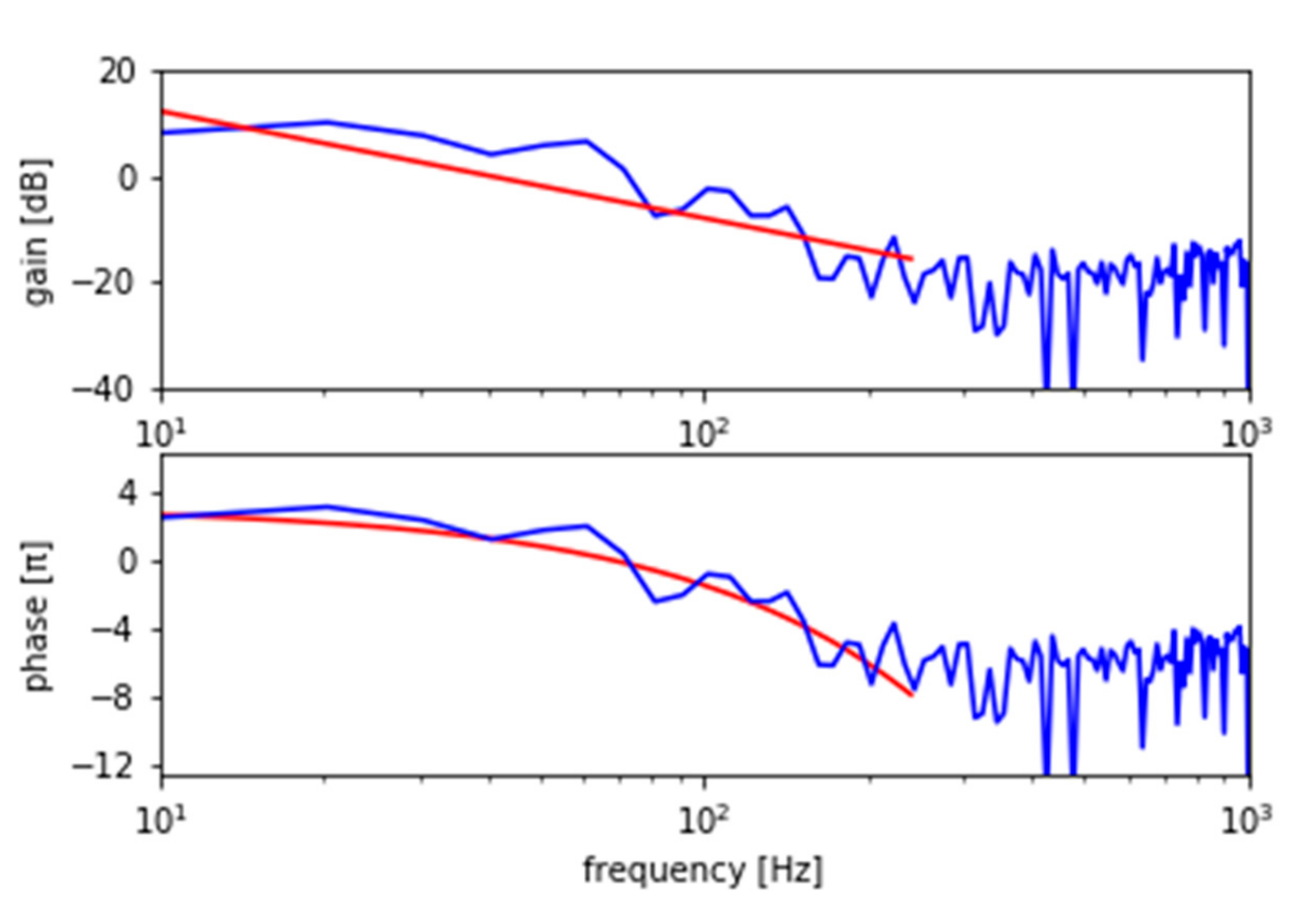
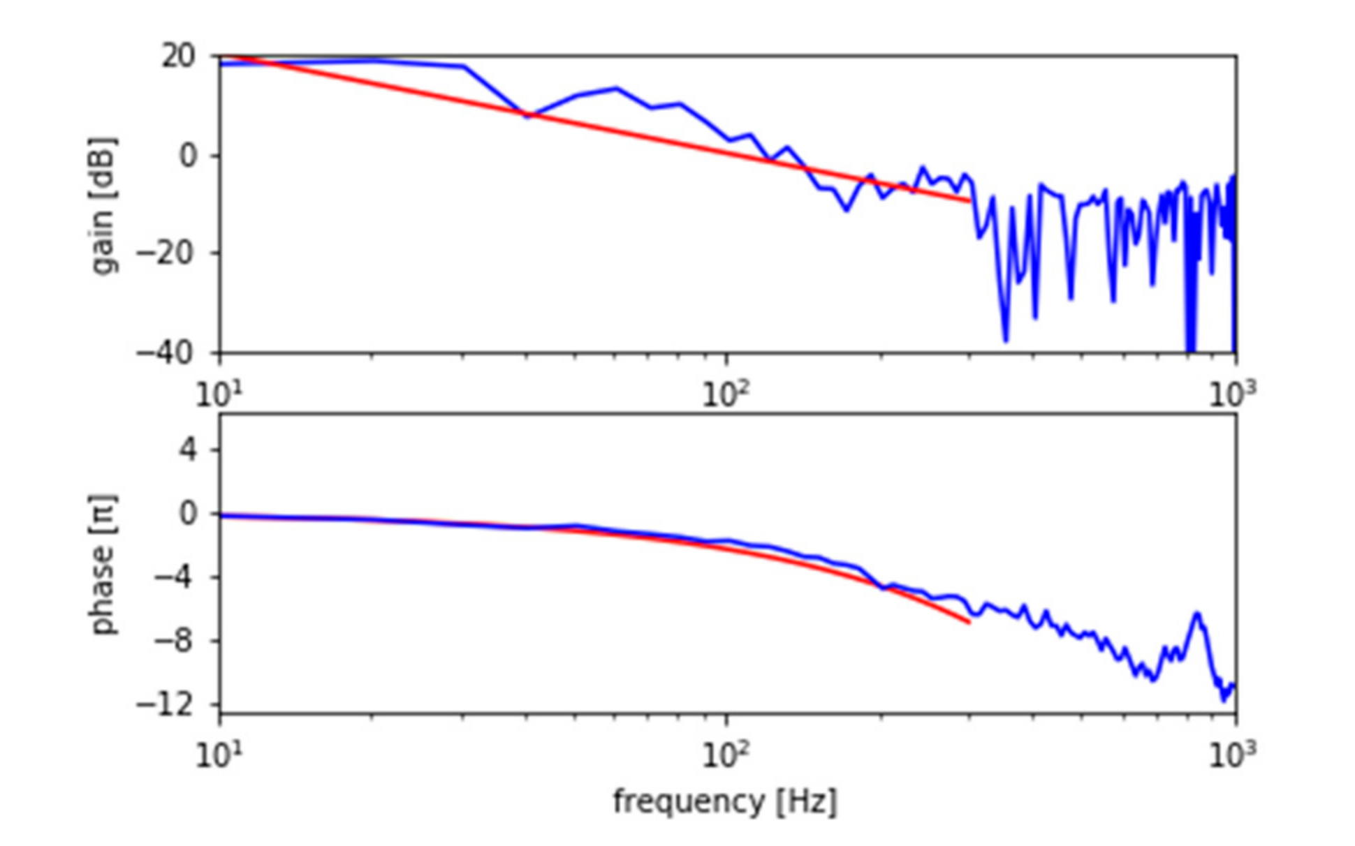
The FTF results show that both flames behave as if the systems have proportional, inertial, and delay components. The time delays, which are simply estimated by curve fitting, indicate that the fluctuating flame fronts are shear layer flame fronts.

(2)

The shedding wake motion (BVK instability) and shear layer motion (KH instability) can then be captured from the POD post-processing method. The results indicate that the dominant frequencies of wake motion are different from those predicted using the literature method.

(3)

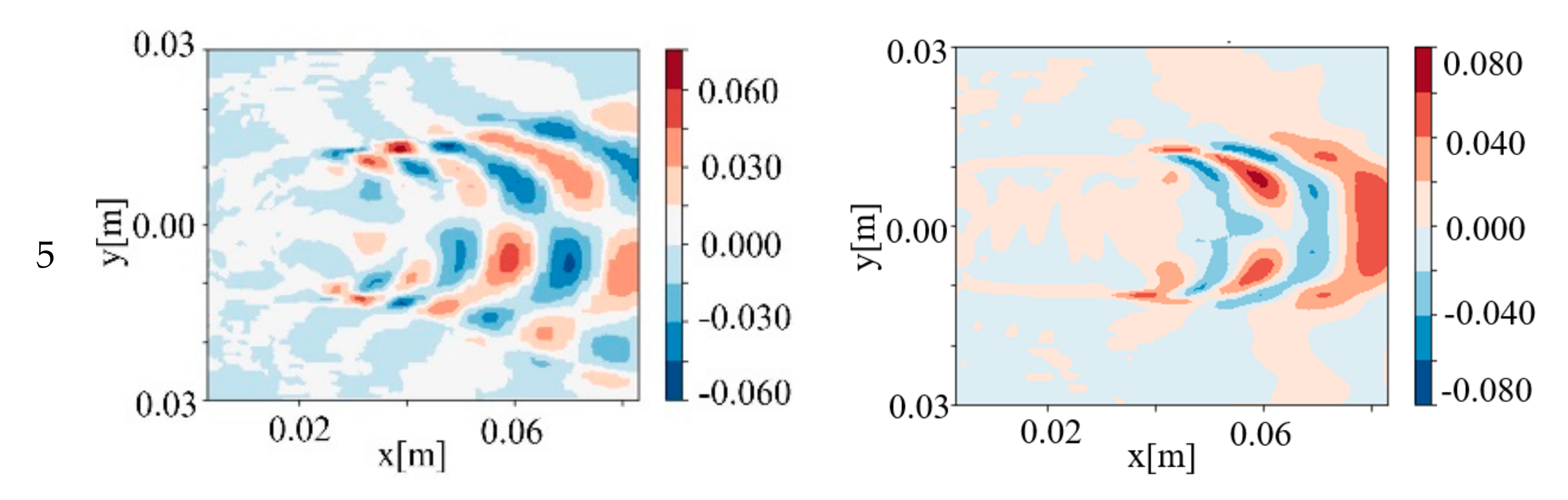
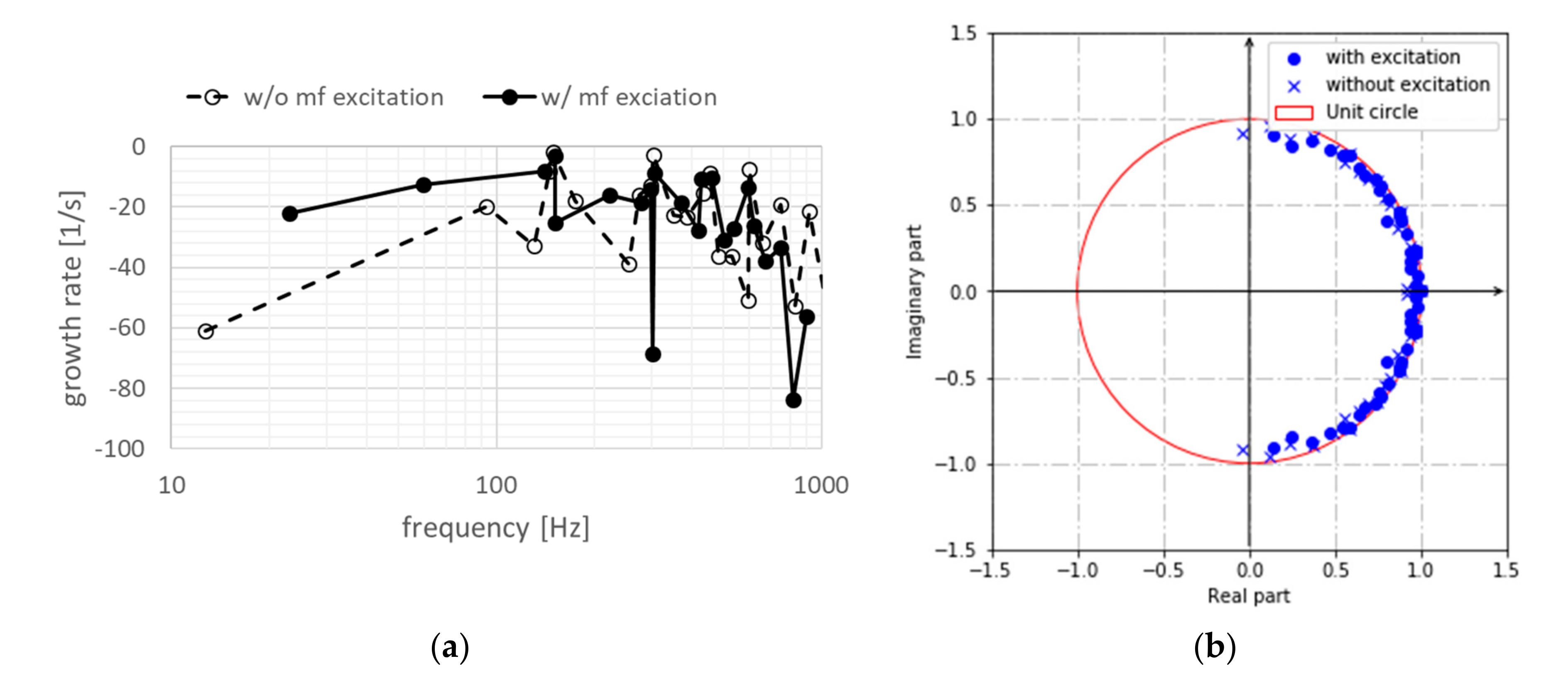
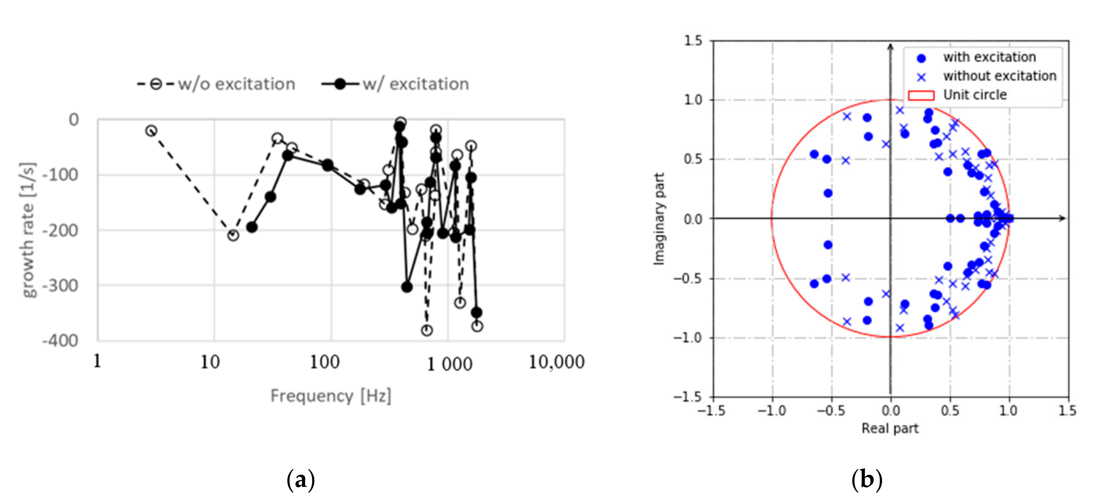
Subsequently, the DMD method was performed. In order to understand which flame structures are responding, with and without inlet excitation, inflow boundary conditions were used for each condition. The excited DMD modes correspond to the shear layer flames swing and convect in the x-direction. Other DMD modes, which have a higher growth rate, are found to be in agreement with the first several POD modes.

(4)

Making a comparison between two inflow conditions, the negative growth rates for the two conditions confirm that the shear layer stabilized flame (condition 2) is more stable than the flame having wake instability (condition 1).

There are also some thoughts and supplementary information that are not mentioned in the test. So far, POD is a standard procedure for the data analysis of LES. However, POD has its own shortcomings. For a dataset with a strong linear correlation, POD is decomposing data based on the quantity of the covariance. This means that

(1)

POD, which is essentially a dimensionality reduction method, its efficiency depends on the relevance of the selected dataset. For example, in condition 1, if the velocity only field is considered, the first two modes contain more accumulated energy than that for the flame only dataset. When the flame only data are considered, the accumulated energy drops.

(2)

When considering both flow and flame data in the same matrix, the standardization procedure should be taken. Actually, this step helps to eliminate the impact from different units andorder of magnitudes. However, this step has been rarely mentioned in the literature.

(3)

Single POD mode might contain multiple flow/flame structures, which are not separated since the variance of such a mode is large. Therefore, the POD cannot be used to distinguish these fine structures.

(4)

Due to uncertainty of the physical significance of higher order POD modes, only the first five modes are shown in this paper. The reason is that the point of inflection is already present in the scree plot. In the analysis, a cumulative variance contribution rate of 80% is considered.

Therefore, from the author’s point of view, it is recommended to use DMD and FTF together to analyze flame dynamics. Even though DMD yields more computational memory and time compared to POD, DMD proposes clear frequency bands, which can be compared with the FTF results. DMD also provides a direct conclusion as to whether the flame structures are stable or not.

The current paper aims at developing joint post-processing procedures and also studied if the V-gutter flame holder can be further developed as the component in the gas turbine combustor. As the results indicated that the flame dynamics are in the very low frequency range, combustor design should be carefully designed to avoid those frequency bands. The test rig should also consider the structure tolerance for such frequency bands.

References

1. Schlein, B.C.; Anderson, D.A.; Beukenberg, M.; Mohr, K.D.; Leiner, H.L.; Träptau, W. Development history and field experiences of the first FT8 gas turbine with dry low NOx combustion system. In Proceedings of the Turbo Expo: Power for Land, Sea, and Air, Indianapolis, IN, USA, 7–10 June 1999. [Google Scholar]
2. Peter, B.; Hoffmann, S. Suppression of dynamic combustion instabilities by passive and active means. In Proceedings of the Turbo Expo: Power for Land, Sea, and Air, Munich, Germany, 8–11 May 2000. [Google Scholar]
3. Strutt, J. The Theory of Sound (Cambridge Library Collection—Physical Sciences); Cambridge University Press: Cambridge, UK, 2011. [Google Scholar]
4. Sundaram, S.S.; Babu, V. Numerical Investigation of Combustion Instability in a V-Gutter Stabilized Combustor. J. Eng. Gas Turbines Power 2013, 135, 501–510. [Google Scholar] [CrossRef]
5. Lieuwen, T.C.; Vigor, Y. Combustion Instabilities in Gas Turbine Engines: Operational Experience, Fundamental Mechanisms, and Modeling; American Institute of Aeronautics and Astronautics: Reston, VA, USA, 2005. [Google Scholar]
6. Bloxsidge, G.J.; Dowling, A.P.; Langhorne, P.J. Reheat buzz: An acoustically coupled combustion instability. part 2. Theory. J. Fluid Mech. 1988, 193, 445–473. [Google Scholar] [CrossRef]
7. Dowling, A.P. The calculation of thermoacoustic oscillations. J. Sound Vib. 1995, 180, 557–581. [Google Scholar] [CrossRef]
8. Lacombe, R.; Föller, S.; Jasor, G.; Polifke, W.; Aurégan, Y.; Moussou, P. Identification of aero-acoustic scattering matrices from large eddy simulation: Application to whistling orifices in duct. J. Sound Vib. 2013, 332, 5059–5067. [Google Scholar] [CrossRef]
9. Schuermans, B.; Guethe, F.; Pennell, D.; Guyot, D.; Paschereit, C.O. Thermoacoustic modeling of a gas turbine using transfer functions measured under full engine pressure. J. Eng. Gas Turbines Power 2010, 132, 503–514. [Google Scholar] [CrossRef]
10. Noiray, N.; Durox, D.; Schuller, T.; Candel, S. Self-induced instabilities of premixed flames in a multiple injection configuration. Combust. Flame 2006, 145, 435–446. [Google Scholar] [CrossRef]
11. Durox, D.; Schuller, T.; Candel, S. Combustion dynamics of inverted conical flames. Proc. Combust. Inst. 2005, 30, 1717–1724. [Google Scholar] [CrossRef]
12. Huber, A.; Polifke, W. Dynamics of Practical Premixed Flames, Part I: Model Structure and Identification. Int. J. Spray Combust. Dyn. 2009, 1, 199–228. [Google Scholar] [CrossRef]
13. Biagioli, F.; Wysocki, S.; Alemela, R.; Srinivasan, S.; Denisov, A. Experimental and LES analysis of a premix swirl burner under acoustic excitation. In Proceedings of the ASME Turbo Expo: Turbomachinery Technical Conference and Exposition Charlotte, Charlotte, NC, USA, 26–30 June 2017. [Google Scholar]
14. Biagioli, F.; Lachaux, T.; Narendran, S. Investigation of the Dynamic Response of Swirling Flows Based on LES and Experiments. Flow Turbul. Combust. 2014, 93, 521–536. [Google Scholar] [CrossRef]
15. Biagioli, F.; Guethe, F. Effect of pressure and fuel-air unmixedness on NOx emissions from industrial gas turbine burners. Combust. Flame. 2007, 151, 274–288. [Google Scholar] [CrossRef]
16. Biagioli, F.; Paikert, B.; Genin, F.; Noiray, N.; Bernero, S.; Syed, K. Dynamic response of turbulent low emission flames at different vortex breakdown conditions. Flow Turbul. Combust. 2013, 90, 343–372. [Google Scholar] [CrossRef]
17. Dolan, B.J.; Gomez, R.V.; Zink, G.; Pack, S.; Gutmark, E.J. High-Speed imaging of combustion oscillations in a multiple nozzle staged combustor. In Proceedings of the 53rd AIAA Aerospace Sciences Meeting, Kissimmee, FL, USA, 5–9 January 2015. [Google Scholar]
18. Huang, C.; Anderson, W.E.; Harvazinski, M.E.; Sankaran, V.S. Analysis of self-excited combustion instabilities using decomposition techniques. AIAA J. 2016, 54, 2791–2807. [Google Scholar] [CrossRef]
19. Wysocki, S.; Syed, K.J.; Biagioli, F. Frequency response of turbulent partially premixed flame stabilized in free-standing vortex breakdown. Combust. Sci. Technol. 2019, 191, 797–832. [Google Scholar] [CrossRef]
20. Schmid, P.; Sesterhenn, J. Dynamic Mode Decomposition of numerical and experimental data. J. Fluid Mech. 2008, 656, 5–28. [Google Scholar] [CrossRef] [Green Version]
21. Rowley, C.W.; MeziĆ, I.; Bagheri, S.; Schlatter, P.; Henningson, D.S. Spectral analysis of nonlinear flows. J. Fluid Mech. 2009, 641, 115–127. [Google Scholar] [CrossRef] [Green Version]
22. Wang, Y.; Son, J.; Sohn, C.H.; Yoon, J.; Bae, J.; Yoon, Y. Combustion Instability Analysis of a Model Gas Turbine by Application of Dynamic Mode Decom-position. J. Korean Combust. 2019, 24, 51–56. [Google Scholar] [CrossRef]
23. Palies, P.; Ilak, M.; Cheng, R. Transient and limit cycle combustion dynamics analysis of turbulent premixed swirling flames. J. Fluid Mech. 2017, 830, 681–707. [Google Scholar] [CrossRef]
24. Wilhite, J.M.; Dolan, B.J.; Gomez, R.V.; Kabiraj, L.; Gutmark, E.J. Analysis of combustion oscillations in a staged MLDI burner using decomposition methods and recurrence analysis. In Proceedings of the 54th AIAA Aerospace Sciences Meeting, San Diego, CA, USA, 4–8 January 2016. [Google Scholar]
25. Ebrahimi, H. Overview of gas turbine augmentor design, operation, and combustion oscillation. In Proceedings of the 42nd AIAA/ASME/SAE/ASEE Joint Propulsion Conference and Exhibit, Sacramento, CA, USA, 9–12 July 2006. [Google Scholar]
26. Lovett, J.; Brogan, T.; Philippona, D.; Keil, B.; Thompson, T. Development needs for advanced afterburner designs. In Proceedings of the 40th AIAA/ASME/SAE/ASEE Joint Propulsion Conference and Exhibit, Fort Lauderdale, FL, USA, 11–14 July 2004. [Google Scholar]
27. Hanbhogue, S.J.; Husain, S.; Lieuwen, T. Lean blowoff of bluff body stabilized flames: Scaling and dynamics. Prog. Energy Combust. Sci. 2009, 35, 98–120. [Google Scholar] [CrossRef]
28. Cardell, G.S. Flow Past a Circular Cylinder with a Permeable Splitter Plate. Ph.D. Thesis, California Insititute of Technology, Pasadena, CA, USA, 1993. [Google Scholar]
29. Lieuwen, T.; Shanbhogue, S.; Khosla, S.; Smith, C. Dynamics of Bluff Body Flames Near Blowoff. In Proceedings of the 45th AIAA Aerospace Sciences Meeting, Reno, NV, USA, 8–11 January 2007. [Google Scholar]
30. Smith, C.; Nickolaus, D.; Leach, T.; Kiel, B.; Garwick, K. LES blowout analysis of premixed flow past v-gutter flameholder. In Proceedings of the 45th AIAA Aerospace Sciences Meeting, Reno, NV, USA, 8–11 January 2007. [Google Scholar]
31. Bothien, M.; Demian, L.; Yang, Y.; Alessandro, S. Reconstruction and analysis of the acoustic transfer matrix of a reheat flame from large-eddy simulations. J. Eng. Gas Turbines Power 2019, 141, 021018. [Google Scholar] [CrossRef]
32. Yang, Y.; Noiray, N.; Scarpato, A.; Schulz, O.; Bothien, M. Numerical analysis of the dynamic flame response in alstom reheat combustion systems. In Proceedings of the ASME Turbo Expo 2015: Turbine Technical Conference and Exposition, Montreal, QC, Canada, 15–19 June 2015. [Google Scholar]
33. Sirovich, L. Turbulence and the dynamics of coherent structures. Part I: Coherent structures. Q. Appl. Math. 1987, 45, 561–571. [Google Scholar] [CrossRef] [Green Version]
34. Chong, T.W.; Komarek, T.; Kaess, R.; Föller, P. Identification of Flame Transfer Functions from LES of a Premixed Swirl Burner; ASME Turbo Expo: Glasgow, UK, 18 June 2010. [Google Scholar]
35. Lennart, L. System Identification: Theory for the User, 2nd ed.; Pearson: Upper Saddle River, NJ, USA, 1999. [Google Scholar]
36. Celik, I.; Klein, M.; Janicka, J. Assessment measures for engineering LES applications. J. Fluids Eng. 2009, 131, 031102. [Google Scholar] [CrossRef]
37. Pope, S.B. Ten Questions Concerning the Large-Eddy Simulation of Turbulent Flows. New J. Phys. 2004, 6, 35. [Google Scholar] [CrossRef] [Green Version]
38. Geurts Bernard, J. A framework for predicting accuracy limitations in large-eddy simulation. Phys. Fluids 2002, 14, L41–L44. [Google Scholar] [CrossRef] [Green Version]
39. Celik, I.B.; Cehreli, Z.N.; Yavuz, I. Index of Quality for Large Eddy Simulations. J. Fluids Eng. 2005, 127, 949–958. [Google Scholar] [CrossRef]
40. Klein, M. An Attempt to Assess the Quality of Large Eddy Simulations in the Context of Implicit Filtering. Flow Turbul. Combust. 2005, 75, 131–147. [Google Scholar] [CrossRef]
41. Wang, S.; Hsieh, S.-Y.; Vigor, Y. Unsteady flow evolution in swirl injector with radial entry. I. Stationary conditions. Phys. Fluids. 2005, 17, 045106. [Google Scholar] [CrossRef] [Green Version]
42. Davidson, L. Large Eddy Simulations: How to evaluate resolution. Int. J. Heat Fluid Flow 2009, 30, 1016–1025. [Google Scholar] [CrossRef] [Green Version]
43. Freitag, M.; Klein, M. Direct Numerical Simulation of a Recirculating, Swirling Flow. Flow Turbul. Combust. 2005, 75, 51–66. [Google Scholar] [CrossRef]
44. Berkeley Mechnical Engineering. Available online: http://www.me.berkeley.edu/gri_mech/ (accessed on 12 June 2019).
45. Zimont, V.; Lipatnikov, A.N. A numerical model of premixed turbulent combustion of gases. Chem. Phys. Rep. 1995, 14, 993–1025. [Google Scholar]
46. Zimont, V.; Polifke, W.; Bettelini, M.; Weisenstein, W. An efficient computational model for premixed turbulent combustion at high Reynolds numbers based on a turbulent flame speed closure. J. Eng. Gas Turbines Power. 1998, 120, 526–532. [Google Scholar] [CrossRef]
47. Yang, Y.; Liu, X.; Zhang, Z.H. Large eddy simulation calculated flame dynamics of one F-class gas turbine combustor. Fuel 2020, 261, 116451. [Google Scholar] [CrossRef]
48. Eriksson, P. The Zimont TFC model applied to premixed bluff body stabilized combustion using four different RANS turbulence models. In Proceedings of the Turbo Expo: Power for Land, Sea, and Air, Montreal, QC, Canada, 14–17 May 2007. [Google Scholar]
Figure 1. Simulation domain.
Energies 13 04886 g001
Figure 2. The largest location where the energy is resolved less than 0.85 is the leading edge of the V-gutter.
Energies 13 04886 g002
Figure 3. Inlet excitation signal. (a) Time series and power spectrum density (PSD). (b) Linear autocorrelation of the inlet excitation signal.
Energies 13 04886 g003
Figure 4. Comparison of the axial average velocity profile for the experimental data, RSM model, k-ε model, and large-eddy simulation (LES) results (LES results are from this work, while other data are extracted from [48]. Left: x = 0.15 m section; Right: x = 0.376 m section).
Energies 13 04886 g004
Figure 5. Comparison of the average temperature profile for the experimental data, the RSM model, the k-ε model, and the LES results (LES results are performed in this work, while other data are extracted from [48]. Left: x = 0.15 m section; Right: x = 0.35 m section).
Energies 13 04886 g005
Figure 6. Production reaction rate contour plots for low (condition 1) and high inlet velocity (condition 2) conditions.
Energies 13 04886 g006
Figure 7. Average field and the corresponding RMS results for condition 1.
Energies 13 04886 g007aEnergies 13 04886 g007b
Figure 8. Average field and RMS result for condition 2.
Energies 13 04886 g008aEnergies 13 04886 g008b
Figure 9. The first five proper orthogonal decomposition (POD) modes in the two conditions.
Energies 13 04886 g009aEnergies 13 04886 g009b
Figure 10. Lissajous plots in condition 1. (a) Scatter plot of the 1st and 2nd modes; the red line represents the unit circle. (b) Scatter plot of the 1st and 4th modes; the red line represents the theoretical line.
Energies 13 04886 g010
Figure 11. Lissajous plots for condition 2. (a) Scatter plot of the 2nd–3rd modes; (b) Scatter plot of the 2nd and 4th modes; (c) Scatter plot of the 2nd and 5th modes; the red line represents the theoretical line.
Energies 13 04886 g011
Figure 12. Bode plot for condition 1.
Energies 13 04886 g012
Figure 13. (a) Eigenvalues with and without excitation in condition 1. (b) Eigenvalues and the unit circle.
Energies 13 04886 g013
Figure 14. The real part of the selected DMD modes in condition 1.
Energies 13 04886 g014aEnergies 13 04886 g014b
Figure 15. Bode plot of condition 2.
Energies 13 04886 g015
Figure 16. (a) Eigenvalues with and without excitation in condition 2. (b) Eigenvalues and unit circle (right).
Energies 13 04886 g016
Figure 17. The real part of the selected DMD modes in condition 2.
Energies 13 04886 g017