Article

Ultra-Short-Term Load Demand Forecast Model Framework Based on Deep Learning

School of Economics and Management, North China Electric Power University, Beijing 102206, China
*
Author to whom correspondence should be addressed.
Energies 2020, 13(18), 4900; https://doi.org/10.3390/en13184900
Submission received: 3 August 2020 / Revised: 5 September 2020 / Accepted: 11 September 2020 / Published: 18 September 2020
(This article belongs to the Section A1: Smart Grids and Microgrids)

Abstract

:
Ultra-short-term load demand forecasting is significant to the rapid response and real-time dispatching of the power demand side. Considering too many random factors that affect the load, this paper combines convolution, long short-term memory (LSTM), and gated recurrent unit (GRU) algorithms to propose an ultra-short-term load forecasting model based on deep learning. Firstly, more than 100,000 pieces of historical load and meteorological data from Beijing in the three years from 2016 to 2018 were collected, and the meteorological data were divided into 18 types considering the actual meteorological characteristics of Beijing. Secondly, after the standardized processing of the time-series samples, the convolution filter was used to extract the features of the high-order samples to reduce the number of training parameters. On this basis, the LSTM layer and GRU layer were used for modeling based on time series. A dropout layer was introduced after each layer to reduce the risk of overfitting. Finally, load prediction results were output as a dense layer. In the model training process, the mean square error (MSE) was used as the objective optimization function to train the deep learning model and find the optimal super parameter. In addition, based on the average training time, training error, and prediction error, this paper verifies the effectiveness and practicability of the load prediction model proposed under the deep learning structure in this paper by comparing it with four other models including GRU, LSTM, Conv-GRU, and Conv-LSTM.

1. Introduction

At present, the power system reform in China is underway, and the spot market in pilot provinces such as Guangdong and Zhejiang will be implemented [1]. Since the electricity spot market has the characteristics of complex trading varieties, high trading frequency, and fluctuating price, the forecasting level of ultra-short-term load is significant. It can help power market members make trading decisions in the energy market, capacity market, auxiliary service market, and demand-side response market [2]. Additionally, ultra-short-term load forecasting is beneficial to arrange the operation mode of a power network and the maintenance plan of a unit reasonably, and can improve the economic and social benefits of a power system.
Load forecasting methods are divided into two categories: Classical statistical forecasting technologies and intelligent forecasting technologies. Classical load forecasting methods mainly include exponential sliding average [3], linear regression [4], auto-regressive integrated moving average [5,6], the dynamic regression method [7], and generalized auto-regressive conditional heteroskedastic approach [8]. The prediction model based on statistics has a relatively simple structure and a clear prediction principle, but its prediction accuracy is low, and it is often only applicable to the case with a small amount of data. Based on the machine learning theory, the intelligent forecasting model can fit the nonlinear relationship between complex variables, thus improving the prediction effect. Common intelligent prediction methods include support vector machine technology [9], neural network [10,11], random forest [12], etc. However, these methods have strict requirements on the selection of features, requiring an experienced person to manually select the input features. In addition, these methods require high stability of sample data and take a long time to preprocess. At the same time, the existing shallow intelligent forecasting technologies mentioned above are not suitable for scenarios with a large amount of data. As the data dimension and training depth increase, it is easy to fall into local optimality and overfitting; thus, the stability of prediction cannot be guaranteed. In recent years, with the development of artificial intelligence technology, a large amount of data has been accumulated in the power system, making it possible and necessary to apply intelligent methods such as deep learning for prediction [13] and continuous developing [14,15,16]. In order to improving the accuracy of deep learning network models, some studies usually choose to increase the complexity of models. However, as the number of training parameters increase, the model training time will also increase significantly. As a result, how to build a high-quality deep learning network model has become a research focus.
The main contribution of this paper is to propose an ultra-short-term load forecasting model, in which convolution, long short-term memory (LSTM), and gated recurrent unit (GRU) deep learning algorithms are integrated to predict the next load every 15 min. The convolution layer is mainly used to capture the characteristics of the data space. LSTM and GRU are used to mine the characteristics of the time dimension of the data. The combination of them can improve the feature mining ability of the model. By inputting the time point, temperature, weather condition, and historical 15-min load, after processing by the deep learning network, finally there is the output of a 15-min load curve for three consecutive days in the future. At the same time, this article has found the most suitable hyperparameters for the proposed deep learning framework through repeated debugging of the hyperparameters. The load forecasting model based on deep learning technology proposed in this paper can better process a large amount of historical data and extract key information. In the forecasting process, the nonlinear relationship between load and other data series can be well fitted. At the same time, through comparison with other models, the results show that the model proposed in this paper shows good overall performance in terms of accuracy and training time. As a consequence, this model can reflect the fluctuations of ultra-short-term load in the future properly.
The rest of this paper is organized as follows: Review of applied research on deep learning is shown in Section 2. Then Section 3 introduces the theory involved in the deep learning model. Section 4 introduces the data samples, experimental environments, and the methods for preprocessing the experimental data. Section 5 presents the structure of deep learning model, as well as model super-parameter adjustment and evaluation indicators. Comparison results of different models are demonstrated in Section 6. Finally, Section 7 provides a conclusion and brief discussion and summarizes the whole paper.

2. Literature Review

According to the time scale of forecast, the time span of electric load forecasting can be divided into medium- and long-term load forecasting, short-term load forecasting, and ultra-short-term load forecasting. Among them, ultra-short-term load forecasting refers to load forecasting within one hour, while short-term load forecasting refers to daily load forecasting and weekly load forecasting. The main research content of this paper is based on the unit of 15 min in the future, so this paper is a framework of ultra-short-term load demand forecasting based on deep learning.
With the development of computer science and technology, deep learning has gradually penetrated into all fields, and the ability of a neural network to extract data features has been significantly improved. The current ultra-short-term load method based on deep learning involves the LSTM [17,18], GRU [19], recurrent neural network (RNN), and other methods.
However, most of the methods used in the literature are based on the traditional feedforward neural network (FNN), which cannot completely solve the defects that the traditional neural network cannot process, i.e., the related information between sequences. Some studies combine unsupervised training with supervised training for hierarchical feature learning [20]. Hierarchical self-coding is used to learn layer by layer for the mining deep feature [21]. In addition, the convolutional neural network (CNN) has achieved good results in image recognition [22], communication signals [23], and natural language processing [24]. Transforming artificially set feature extraction into automatic generation feature extraction is the biggest advantage of CNN, which also has great prospects for the ultra-short-term load forecast. On the other hand, deep belief neural networks [25,26] and RNN [27,28] have achieved good results in wind speed prediction, photovoltaic power prediction, short-term load, and ultra-short-term load forecast. However, most of the current methods adopted in the literature are based on the traditional feedforward neural network (FNN), which does not completely solve the defect that traditional neural networks cannot process, i.e., the inter-sequence-related information.
In theory, RNN can capture long-distance dependence, but in practice, RNN face two challenges: Gradient explosion and vanishing gradient; so it is difficult for traditional RNN to learn long-term dependencies, while LSTM and GRU solve this problem perfectly. The LSTM network [29] is a type of improved recurrent neural network with the hidden unit replaced by a gated memory cell. LSTM can realize deep memory learning of important information in historical data through state cells and three special gate structures, avoiding the gradient explosion or gradient disappearing that may be caused by general RNNs in the back propagation. As a result, LSTM performs excellently when processing and predicting time series-related data. At present, LSTM networks have been widely used in robot control, text recognition [30], speech recognition [31], protein homology detection, and other fields. In terms of forecast, LSTM has also gradually attracted the attention of scholars [32,33].
Although LSTM has a strong ability to solve long-term dependencies, the parameters of the LSTM network are four times that of the traditional RNN [34], making the model too redundant. In 2014, another gating model, GRU, was proposed, which was applied to language translation for the first time [35], and achieved long-term memory effects with fewer parameters. In recent years, GRU has been gradually applied by scholars in the forecast of traffic flow [36] and energy consumption forecasts [37]. The advantages of LSTM and GRU compared to other models in the direction of load prediction have been fully verified in the literature [38,39].
Therefore, this paper takes the advantages of convolution, LSTM, and GRU in processing time series data and introduces convolution to avoid overfitting. By experimenting with the load data from the user side of a city in Northern China, the feasibility of the deep neural network framework is verified.

3. Theoretical Description of the Proposed Model

The deep learning structure proposed in this paper mainly contains two parts: The functions of convolution are feature extraction and training parameter reduction to overcome the overfitting problem; LSTM and GRU are introduced to extract features across time steps. Convolution, LSTM, and GRU are three kinds of neural networks with different architectures. This section will introduce more details about these three neural networks.

3.1. Convolution

Convolution is an operation dedicated to processing data with a similar grid structure, working with three important characteristics: Sparse interactions, parameter sharing, and equivariant representations [40,41]. These three advantages make it possible to effectively reduce the complexity of the network and the number of training parameters.
As shown in Figure 1, the neurons are connected to a local area in the input layer, and each neuron calculates the inner product of its own area connected to the input layer and its own weight. Finally, the convolutional layer calculates the output of all neurons. The pooled layer is usually placed behind the convolutional layer and pools the output of the convolution layer.
Different dimensions of convolution filters are used to process different types of data. One-dimensional convolution is often used in sequence models, such as natural language processing; two-dimensional convolution is applied in the field of computer vision and image processing; and three-dimensional convolution is suitable for the medical and video-processing field. The deep learning model framework constructed in this paper uses one-dimensional convolution to process time series data related to electrical load.

3.2. Long Short-Term Memory

The LSTM neural network is a special recurrent neural network (RNN), which introduces a weighted connection with memory and feedback functions. Compared with the feedforward neural network, LSTM can avoid gradient explosion and gradient disappearance, so LSTM can achieve continuous learning for longer time series [42]. The LSTM hidden layer structure is shown in Figure 2. The core of the LSTM is to store the information of the cell state and three different functional gate structures [43], input gate, forget gate, and output gate, and memory cells of the same shape as the hidden state.
The LSTM uses two gates to control the content of the unit state C; one is the forgetting gate, which determines how much unit state is retained to the current moment Ct-1. The other is the input gate, which determines how many inputs X t of the network are saved to the unit state at the current moment. LSTM uses the output gate to control H t value the unit state has compared to the current output value of Ct.
Input gate:
I t = σ ( X t W x i +   H t 1 W h i + b i )
Forgotten door:
F t = σ ( X t W x f +   H t 1 W h f + b f )
Output layer:
O t = σ ( X t W x o + H t 1 W h o + b o )
Calculation of candidate memory cells:
c ˜ t = t a n h ( X t W x c +   H t 1 W h c + b c )
Calculation of memory cells:
c t = F t · c t 1 + i t · c ˜ t
The calculation of the hidden state:
H t = O t · t a n h ( c t )
where Wxi, Wxf, Wxo and Whi, Whf, Who are the weight parameters, bi, bf, bo are the deviation parameters, H t 1 is the output value of the network layer at the previous moment, X t is the current time input value, and I t , F t , O t are the gate structures that control whether the memory unit needs to be updated, whether it needs to be set to 0, and whether it needs to be reflected in the activation vector.

3.3. Gate Recurrent Unit

GRU is another kind of recurrent neural network (RNN). GRU and LSTM are similar in actual performance in many cases. GRU is also proposed to solve problems such as gradients in long-term memory and back propagation. Compared with LSTM, GRU can achieve considerable results, and it is easier to train, which can greatly improve training efficiency [44]. Therefore, GRU tends to be used more in many cases.
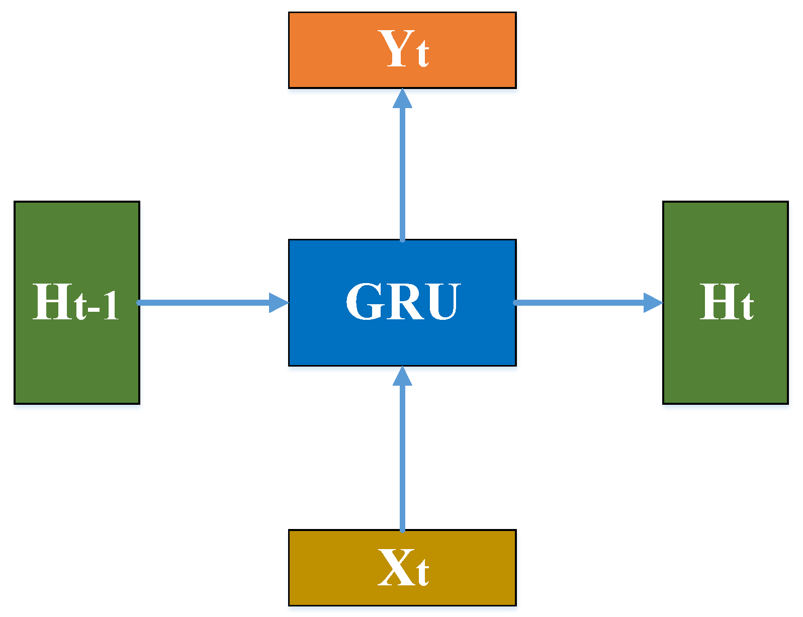
As shown in Figure 3, the structure of the GRU input and output is similar to that of a traditional RNN.
The GRU uses the update gate and the reset gate to update and reset the information. As shown in Equations (1) and (2), the structure is similar to that of the LSTM gate.
The input of the GRU hidden layer:
a j t = f ( i = 1 I w ij   H t 1 + h = 1 H w if   b h t 1 )
The output of the GRU hidden layer:
z j t = f ( i = 1 I w iz   a j t + h = 1 H w io   b f t 1 )
Calculation of memory cells:
c ˜ t = t a n h ( X t W x c +   H t 1 W h c + b c )
The calculation of the hidden state:
H t = z j t · t a n h ( c ˜ t )
where w ij w if , w iz and w io , W x c , W h c are the weight parameters, b h t 1 , b f t 1 , b c are the deviation parameters, H t 1 is the output value of the network layer at the previous moment, X t is the current time input value, and a j t ,   z j t are the gate structures that control whether the memory unit needs to be updated, whether it needs to be set to 0, and whether it needs to be reflected in the activation vector.
Compared with LSTM, the GRU has one less “gating” inside, and the parameters are less than LSTM, but it can also achieve the same function as LSTM. As a result, GRU is more practical sometimes. Therefore, the ability to learn the time series of GRU is greatly superior [45].

4. Data Description

This paper collected three-year load data from Beijing from 2016 to 2018 (sampling interval is 15 min with a total of 105,163 points of data) and meteorological data (including temperature and weather condition descriptions) as experimental samples. Among them, the temperature data in every 15 min is generated from the highest and lowest temperature data in the day according to the arithmetic relationship. The network training was carried out under the TensorFlow deep learning framework [46], and the Adam optimization algorithm [47] was used to solve the problem. The computer used in the experiment was configured with a 2.2 GHz Intel Core i7 processor and 16 GB 1600 MHz DDR3 memory.

4.1. Feature Engineering

Traditional machine learning methods such as SVM, shallow neural networks, etc., rely on the experience of the relevant staff to manually construct features when building models, while deep neural networks are an end-to-end training that automatically extracts sample data features and can greatly improve work efficiency. This paper combines deep convolution, LSTM, and GRU to simplify the construction of sample features. Because the deep neural network can capture general periodicity of features, this paper therefore no longer selects forecast day types (workdays or weekends) as input features. The high precision of the experimental results indicates that the combination of convolution, LSTM, and GRU has fully extracted the features in the sample data.
According to the collected raw data, the input and output of the model constructed in this paper are shown in Table 1.
A large amount of literatures has only selected temperature as a factor of load for meteorological factors, and has not considered the weather conditions. However, in actual situations, the impact of this condition on the load during the day is very significant. Especially in areas such as Beijing, when extreme weather such as haze occurs, it will have a great impact on the load. It is not sensible to consider the impact on the load from the temperature alone. Therefore, the characteristics of historical weather conditions (such as fog, clouds, etc.) are also considered. There are 18 types, and the text is digitized by using the category features. The information is mapped into a vector, and the conversion result is as shown in Table 2.

4.2. Data Preprocessing

In the data preprocessing stage, in order to eliminate the influence of different physical dimensions, the original data needs to be standardized. This paper uses the Z-score method to standardize all sample data. The formula is as follows:
x ^ ( i ) = x ( i ) x m e a n x s t a n d a r d   d e v i a t i o n  
For modeling and calculation, the basic unit of measure is the same, the neural network is trained (probabilistic calculation) and predicted by the statistical probability of the sample in the event, and the value of the Sigmoid function is between 0 and 1. The output of the last node is the same. Where x ^ ( i ) represents the normalized data value, and the mean and standard deviation of the original samples, respectively, where weather condition assignment refers to the mapping results of Table 2. The first five rows of the data preprocessing result are shown in Table 3.

5. Deep Learning Model

5.1. Deep Learning Network Prediction Framework

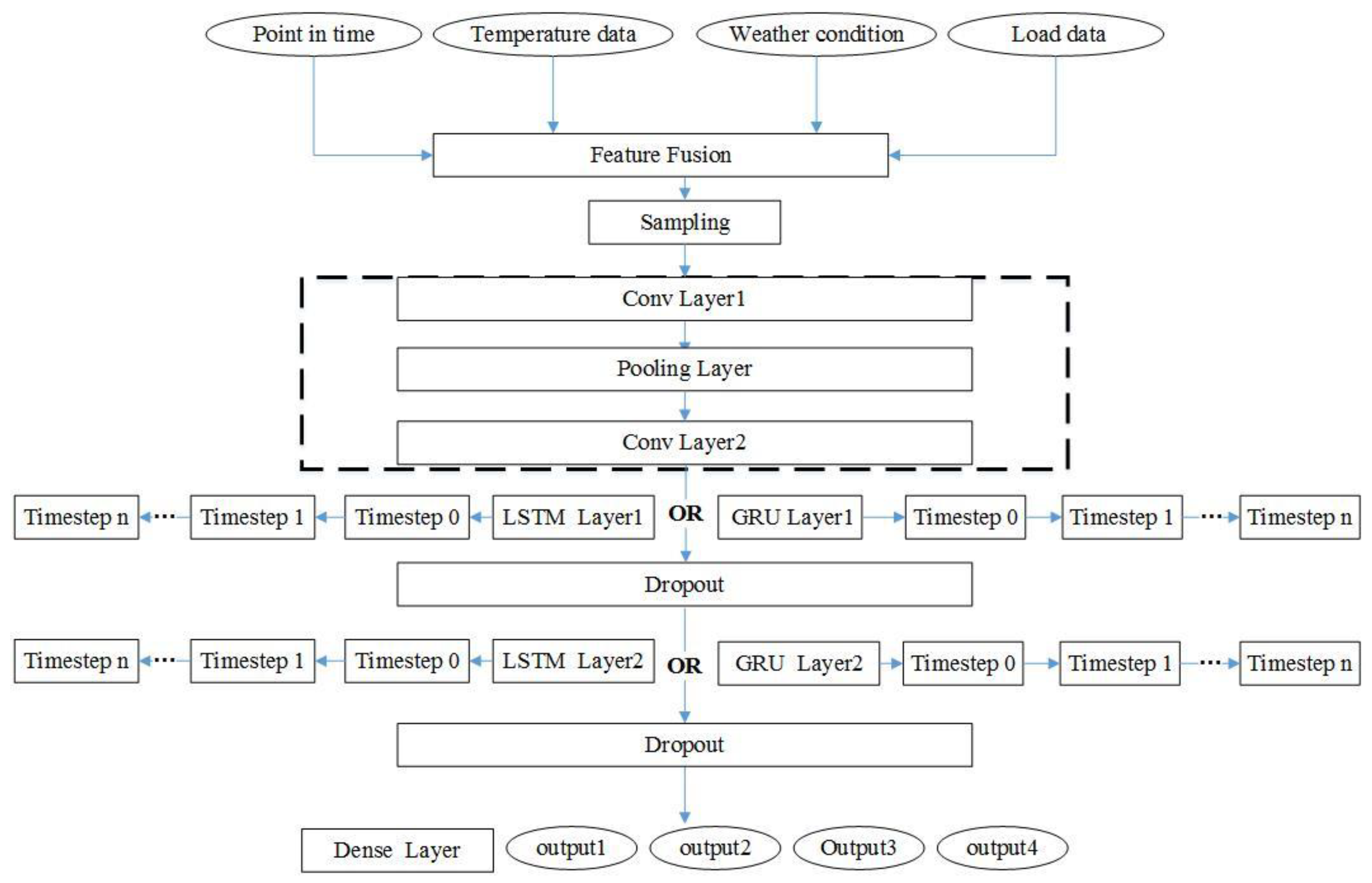
The deep learning framework constructed in this paper consists of two convolutional layers, one LSTM layer and one GRU layer.
As the Figure 4 shows, firstly, the historical meteorological data and the load data are pre-processed and combined, and then the overall time series is sampled. Then, the convolution filter is used to extract higher-order sample features and reduce the number of training parameters. The Relu function [21] is used as the activation function. Next, the LSTM layer or GRU layer is used for time series-based modeling, and the dropout layer is introduced after each layer to reduce the risk of overfitting. Finally, the load prediction result is output by a dense layer.
The overall construction process of this deep learning model is as follows:
Step 1: Data preprocessing.
The input characteristics of a single moment is 4 (see in Table 1) with a total of 105,163 training samples. Time step and batch size are adjustable hyperparameters, so the input data is stored in a 3-dimensional tensor (batch size * Time step * 4).
Step 2: Model training.
Eighty percent of the sample data is set as the training set, 20% of the sample data is set as the test set, then the processed training set data is input into the deep learning model for training. Then model outputs the next four consecutive 15 min, which is one hour of load forecast.
Step 3: Adjust the model hyperparameters.
Continue to optimize the model and compare the accuracy using different hyperparameters models.

5.2. Hyperparameters of Deep Learning Model

In order to obtain the optimal structure of the above deep learning model, this paper uses the vertical comparison method to adjust the parameters of the number of hidden layer nodes, time step, and batch size of the improved RNN. When analyzing the influence of one of the parameters on the prediction result, the remaining parameters are fixed. The parameters selected throughout the experimental process are shown in the following Table 4:
In this paper, mean square error (MSE) is used for error evaluation. The expressions are as follows:
δ M S E = 1 n i = 1 n ( y i y ^ i ) 2  
MSE is a convenient method to measure the “average error “. MSE can evaluate the degree of change of the data. The smaller the value of the MSE, the better the accuracy of the prediction model to describe the experimental data. Where y i represents the actual load value, y ^ i represents the load forecast value, and n represents the number of load forecast points. The value of n in this deep learning model is 4.
According to Figure 5, the epoch of the training process is 5, and each training basically converges in the second epoch model. According to the trend in the figure, it can be seen that the overall error of the model is decreasing, and the error is already in the acceptable range.
The final experimental scene has a tendency to fit, so the model training is stopped, and the optimal model parameters are obtained as shown in Table 5.

5.3. Evaluation Index

In order to test the prediction effect of the model, it is necessary to select the appropriate evaluation criteria. This paper uses the coefficient of determination to evaluate, denoted by R 2 , and the expression is as follows:
R 2 =   i = 1 n ( y ^ i y i ¯ ) 2 i = 1 n ( y y i ¯ ) 2
R 2 is generally the best measure of linear regression, usually indicating the quality of the model. R 2 ranges between 0 and 1; the closer to 1, the better. y i represents the actual load value, y ^ i represents the load forecast value, y i ¯ represents the actual load average, and n represents the number of load forecast points. The closer R 2 is to 1, the higher the goodness of fit is.

6. Results

In order to verify the superiority of the proposed model, this section describes the model training process in detail. The model proposed in this paper is compared with the other four deep learning models, and the details of models are as follows, in which model 5 is the abbreviation of the model proposed in this paper:
Model 1 (GRU): The preprocessed data is input to the GRU layer directly, without using a convolution filter layer. GRU layer hidden layer unit is 50;
Model 2 (LSTM): The preprocessed data is input to the LSTM layer directly, without using a convolutional layer for filtering. LSTM layer hidden layer unit is 50;
Model 3 (Conv-LSTM): The preprocessed data is input to the convolutional layer firstly for filtering, and then two LSTM layers are used for prediction. Kernel size in Conv Layer is 4 × 4. LSTM layer hidden layer unit is 50;
Model 4 (Conv-GRU): The preprocessed data is input to the convolutional layer firstly for filtering, and then two GRU layers are used for prediction. Kernel size in Conv Layer is 4 × 4. GRU layer hidden layer unit is 50;
Model 5 (Conv-GRU-LSTM): The preprocessed data is input to the convolutional layer firstly for filtering, and then a GRU layer and an LSTM layer are used for prediction. Kernel size in Conv Layer is 4 × 4. GRU and LSTM layer hidden layer unit is 50.

6.1. Training Process Analysis

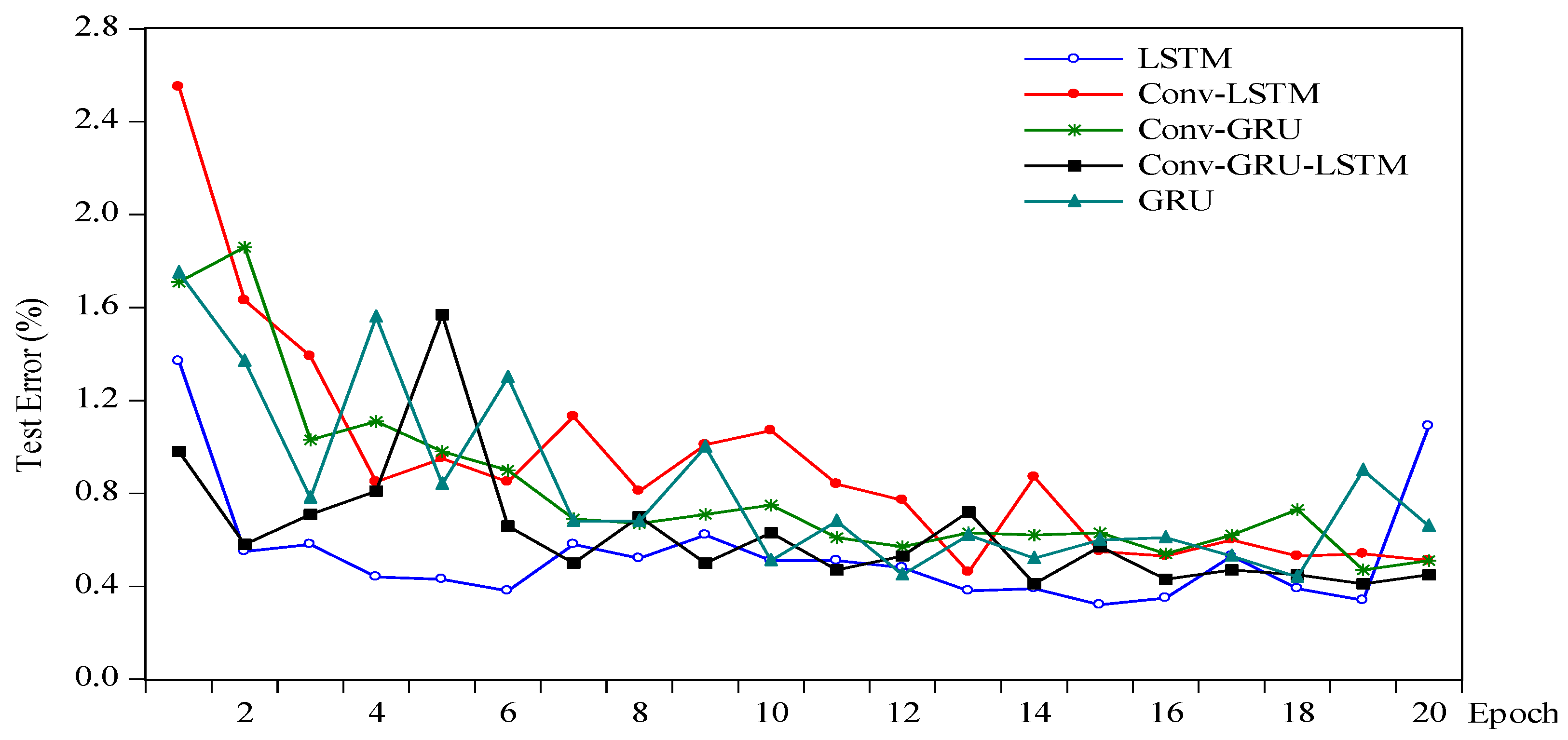
In order to reflect the superiority of the proposed deep learning framework, the other two deep learning model without convolutional layer are introduced to compare with three models constructed in the framework. The five models are all trained using the optimal parameters obtained in Table 5, and the epoch was set to 20. Training time and accuracy of the five models are demonstrated as follows.
According to Figure 6, it can be seen whether the introduction of convolution has a great training time for deep neural networks in terms of training time, which is positively related to the number of parameters that need to be trained. Conv-GRU had the shortest training time in the five models, LSTM had the longest training time, LSTM training time was almost five times that of Conv-LSTM, and GRU training time was more than three times that of Conv-GRU.
According to Figure 7, as the training deepens, both the LSTM and GRU models have a tendency to overfit, which may be due to the complexity of the training parameters, while the Conv-LSTM, Conv-GRU, and Conv-GRU-LSTM become more and more stable. This is because the deep learning framework proposed in this paper can greatly reduce the parameters that need to be trained while ensuring the accuracy of prediction, and ultimately reducing the cost of model training time.

6.2. Forecast Results Display

In order to further verify the superiority of the deep learning framework of this paper, the five models are used to predict the 288 consecutive point loads in the last three days in 2018. The prediction results, error, and R2 are shown in Figure 8 and Figure 9 and Table 6. The expression of error is as follows:
Error = ( predicted   value real   value ) / real   value
As Figure 8 shows, the five deep learning models generally have splendid prediction accuracy and strong stability, proving the feasibility of applying the deep learning method to ultra-short-term load forecast. Through the calculation of R2 value, the results of the five deep learning models were all greater than 0.9. Conv-LSTM had the best goodness of fit, and Conv-GRU-LSTM had the second goodness of fit, which further proves the superiority of the deep learning framework proposed in this paper.
According to the experimental results, although the Conv-LSTM model had the highest coefficient of determination (0.9705), judging from the model training time in Figure 6, the training time of the Conv-GRU-LSTM model was much lower than that of the Conv-LSTM model. Therefore, comprehensively considering, the Conv-GRU-LSTM model was more practical. Especially when dealing with a large amount of sample data, the superiority of the model proposed in this paper is even more significant.

7. Conclusions and Discussion

7.1. Conclusions

With the acceleration of the power market reform process, the importance of ultra-short-term load forecasting for grid companies and emerging purchase and sale companies is becoming more apparent. At the same time, affected by many uncertain factors, the future load changes present uncertainty. In comparison with the traditional point forecasting method, the deep learning framework can actively mine the hidden information in historical data, which is conducive to the decision-making and execution of electricity purchase and sale strategies of each power trading subject, and further promotes the economics of electricity market trading.
When using large-scale data for load forecasting, the conventional prediction method always leads to an excessively complicated model and an excessive computational cost in the training process. In this paper, convolution was combined with LSTM and GRU to construct Conv-GRU-LSTM ultra-short-term load forecast models. The main research conclusions are as follows:
(1) With the use of power system big data, this paper collected more than 100,000 historical load data, making full use of the advantages of deep learning neural network to automatically extract features, simplifying the input features and reducing the process of manual construction features. The coefficient of determination of the Conv-GRU-LSTM model is 0.9639, which is very close to 1. Considering the comprehensive training time, the final experimental results show that the learning framework combining convolution with LSTM and GRU has excellent ability of feature mining.
(2) The model proposed in this paper is compared with the other four models including GRU, LSTM, Conv-GRU, and Conv-LSTM. The results show that the Conv-GRU-LSTM model proposed in this paper presents comprehensive advantages in training time and prediction accuracy.
(3) This paper aims at the short-term load forecasting in the next few minutes. The input sample has a three-year time span, so the forecasting results will not be affected by seasonal changes. Therefore, the model in this paper can be applied to short-term load forecasting in all periods of the year.

7.2. Discussion

Although the deep learning proposed in this paper can be well applied to forecast ultra-short-term load, there is still room for improvement in this paper. Further research can be carried out in the following two aspects:
(1) The model hyperparameters can be further adjusted, such as hidden layers and number of nodes. Meanwhile, the prediction model of this paper can also be generalized to photovoltaic power generation prediction and wind power prediction through hyperparameter adjusting;
(2) The deep learning framework constructed in this paper can be combined with multi-task learning as well. With reference to migration learning, and the coupling relationship of different energy sources in the integrated energy system, this model can also be introduced to improve the accuracy of multi-load prediction.

Author Contributions

H.L. (Hongze Li) conceived and designed the research method used in this paper; H.L. (Hongyu Liu) writing original draft; H.J. collected the data, related policy documents and reference used for the analysis; P.L. performed the empirical analysis; S.Z. data presentation. All authors have read and agreed to the published version of the manuscript.

Funding

This research received no external funding.

Acknowledgments

The authors greatly appreciate the library of North China Electric Power University for offering related materials. The authors are very grateful to Ruochi Zhang who gave guidance on the research method of this article, and Bingkang Li who provided revision of the language of this article.

Conflicts of Interest

The authors declare no conflict of interest.

References

  1. Luo, X.; Oyedele, L.O.; Ajayi, A.O.; Akinade, O.O. Comparative study of machine learning-based multi-objective prediction framework for multiple building energy loads. Sustain. Cities Soc. 2020, 61, 102283. [Google Scholar] [CrossRef]
  2. Zhang, Z.; Yu, D. RBF-NN based short-term load forecasting model considering comprehensive factors affecting demand response. Proc. CSEE. 2018, 38, 1631–1638. [Google Scholar]
  3. Kang, C.; Xia, Q.; Liu, M. Power System Load Forecasting; Electric Power Press: Beijing, China, 2017. [Google Scholar]
  4. Zhang, F.S.; Wang, H.; Han, T.; Sun, X.Q.; Zhang, Z.Y.; Cao, J. Short-term load forecasting based on partial least-squares regression. Power Syst. Technol. 2003, 3, 36–40. [Google Scholar]
  5. Ramos, P.; Santos, N.; Rebelo, R. Performance of state space and ARIMA models for consumer retail sales forecasting. Robot. Comput. Integr. Manuf. 2015, 34, 151–163. [Google Scholar] [CrossRef] [Green Version]
  6. Chen, P.; Yuan, H.; Shu, X. Forecasting Crime Using the ARIMA Model. In Proceedings of the 2008 Fifth International Conference on Fuzzy Systems and Knowledge Discovery, Shandong, China, 18–20 October 2008; pp. 627–630. [Google Scholar]
  7. Patil, G.R.; Sahu, P.K. Simultaneous dynamic demand estimation models for major seaports in India[J]. Transportation Letters. Int. J. Transp. Res. 2017, 9, 141–151. [Google Scholar]
  8. Garcia, R.; Contreras, J.; Van Akkeren, M.; Garcia, J.B.C. A GARCH forecasting model to predict day-ahead electricity prices. IEEE Trans. Power Syst. 2005, 20, 867–874. [Google Scholar] [CrossRef]
  9. Guzey, H.; Akansel, M. A Comparison of SVM and Traditional Methods for Demand Forecasting in a Seaport: A case study. Int. J. Sci. Technol. Res. 2019, 5, 168–176. [Google Scholar] [CrossRef] [Green Version]
  10. Wang, S.; Zhang, N.; Wu, L.; Wang, Y. Wind speed forecasting based on the hybrid ensemble empirical mode decomposition and GA-BP neural network method. Ren. Energy 2016, 94, 629–636. [Google Scholar] [CrossRef]
  11. Shi, H.; Xu, M.; Li, R. Deep Learning for Household Load Forecasting—A Novel Pooling Deep RNN. IEEE Trans. Smart Grid 2018, 9, 5271–5280. [Google Scholar] [CrossRef]
  12. Chen, M.; Yuan, J.; Liu, D.; Li, T. An adaption scheduling based on dynamic weighted random forests for load demand forecasting. J. Supercomp. 2020, 76, 1–19. [Google Scholar] [CrossRef]
  13. Dedinec, A.; Filiposka, S.; Dedinec, A.; Kocarev, L. Deep belief network based electricity load forecasting: An analysis of Macedonian case. Energy 2016, 115, 1688–1700. [Google Scholar] [CrossRef]
  14. Qing, X.; Chao, Z.; Shuangshuang, Z.; Jian, L.; Dan, G.; Yongchun, Z. Research on Short-term Electric Load Forecasting Method Based on Machine Learning. Electr. Meas. Instrum. 2019, 56, 70–75. [Google Scholar]
  15. Jincheng, F. Research on Short-Term Power Load Forecasting Model Based on DEEP Learning; University of Electronic Science and Technology of China: Chengdu, China, 2020. [Google Scholar]
  16. Yu, G. Application Research of Machine Learning in Short-Term Power Load Forecasting; Anhui University: Hefei, China, 2020. [Google Scholar]
  17. Haican, L.; Weifeng, W.; Bing, Z.; Yi, Z.; Qiuting, G.; Wei, H. Short-term station load forecasting based on Wide&Deep-LSTM model. Power Syst. Technol. 2020, 44, 428–436. [Google Scholar]
  18. Dongfang, Y.; Ying, W.; Lei, L.; Shuai, Y.; Wenguang, W.; Hong, D. Short-term power load forecasting based on deep learning. Foreign Electr. Meas. Technol. 2020, 39, 44–48. [Google Scholar]
  19. Zengping, W.; Bing, Z.; Weijia, J.; Xin, G.; Xiaobing, L. Short-term load forecasting method based on GRU-NN model. Autom. Electr. Power Syst. 2019, 43, 53–62. [Google Scholar]
  20. Wu, R.; Bao, Z.; Song, X.; Deng, W. Research on short-term load forecasting method of power grid based on deep learning. Mod. Electr. Power 2018, 35, 43–48. [Google Scholar]
  21. Wang, K.; Qi, X.; Liu, H. A comparison of day-ahead photovoltaic power forecasting models based on deep learning neural network. Appl. Energy 2019, 251, 113315. [Google Scholar] [CrossRef]
  22. Zhang, W.; Xu, Y.; Ni, J.; Shi, H. Image target recognition algorithm based on multi-scale block convolutional neural network. J. Comput. Appl. 2016, 36, 1033–1038. [Google Scholar]
  23. Wang, P.; Zhao, J.G. New Method of Modulation Recognition Based on Convolutional Neural Networks. Radio Eng. 2019, 9, 453–457. [Google Scholar]
  24. Zhang, C.; Qin, P.; Yin, Y. Adaptive Weight Multi-gram Statement Modeling System Based on Convolutional Neural Network. J. Comput. Sci. 2017, 44, 60–64. [Google Scholar]
  25. Wang, H.Z.; Wang, G.B.; Li, G.Q.; Peng, J.C.; Liu, Y.T. Deep belief network based deterministic and probabilistic wind speed forecasting approach. Appl. Energy 2016, 182, 80–93. [Google Scholar] [CrossRef]
  26. Zhang, X.; Wang, R.; Zhang, T.; Zha, Y. Short-term load forecasting based on a improved deep belief network. In Proceedings of the 2016 International Conference on Smart Grid and Clean Energy Technologies (ICSGCE), Chengdu, China, 19–22 October 2016; Volume 42, pp. 339–342. [Google Scholar] [CrossRef]
  27. Zhang, Y.; Ai, W.; Lin, L.; Yuan, S.; Li, Z. Regional-level ultra-short-term load forecasting method based on deep-length time-time memory network. Power Syst. Technol. 2019, 43, 1884–1892. [Google Scholar]
  28. Hochreiter, S.; Schmidhuber, J. Long Short-Term Memory. Neural Comput. 1997, 9, 1735–1780. [Google Scholar] [CrossRef] [PubMed]
  29. Rao, G.; Huang, W.; Feng, Z.; Cong, Q. LSTM with sentence representations for document-level sentiment classification. Neurocomputing 2018, 308, 49–57. [Google Scholar] [CrossRef]
  30. Sundermeyer, M.; Ney, H.; Schlüter, R. From Feedforward to Recurrent LSTM Neural Networks for Language Modeling. IEEE/ACM Trans. Audio Speech Lang. Process. 2015, 23, 517–529. [Google Scholar] [CrossRef]
  31. Qing, X.; Niu, Y. Hourly day-ahead solar irradiance prediction using weather forecasts by LSTM. Energy 2018, 148, 461–468. [Google Scholar] [CrossRef]
  32. Kong, W.; Dong, Z.; Jia, Y.; Hill, D.J.; Xu, Y.; Zhang, Y. Short-Term Residential Load Forecasting Based on LSTM Recurrent Neural Network. IEEE Trans. Smart Grid 2017, 10, 841–851. [Google Scholar] [CrossRef]
  33. Greff, K.; Srivastava, R.K.; Koutnik, J.; Steunebrink, B.R.; Schmidhuber, J. LSTM: A Search Space Odyssey. IEEE Trans. Neural Netw. Learn. Syst. 2017, 28, 2222–2232. [Google Scholar] [CrossRef] [Green Version]
  34. Chung, J.; Gulcehre, C.; Cho, K.H. Empirical evaluation of gated recurrent neural networks on sequence modeling. arXiv 2014, arXiv:1412.3555. [Google Scholar]
  35. Fu, R.; Zhang, Z.; Li, L. Using LSTM and GRU neural network methods for traffic flow prediction. In Proceedings of the 2016 31st Youth Academic Annual Conference of Chinese Association of Automation (YAC), Wuhan, China, 11–13 November 2016; pp. 324–328. [Google Scholar]
  36. Le, T.-T.-H.; Kim, J.; Kim, H. Classification performance using gated recurrent unit recurrent neural network on energy disaggregation. In Proceedings of the 2016 International Conference on Machine Learning and Cybernetics (ICMLC), Jeju, South Korea, 10–13 July 2016; Volume 1, pp. 105–110. [Google Scholar]
  37. Pezeshki, M. Sequence modeling using gated recurrent neural networks. arXiv 2015, arXiv:1501.00299. [Google Scholar]
  38. Huang, Q.; Wang, W.; Zhou, K. Scene labeling using gated recurrent units with explicit long range conditioning. arXiv 2016, arXiv:1611.07485. [Google Scholar]
  39. Tang, Y.; Huang, Y.; Wu, Z.; Meng, H.; Xu, M.; Cai, L. Question detection from acoustic features using recurrent neural network with gated recurrent unit. In Proceedings of the 2016 IEEE International Conference on Acoustics, Speech and Signal Processing (ICASSP), Shanghai, China, 20–25 March 2016; pp. 6125–6129. [Google Scholar]
  40. Chollet, F. Xception: Deep Learning with Depthwise Separable Convolutions. In Proceedings of the 2017 IEEE Conference on Computer Vision and Pattern Recognition (CVPR), Honolulu, HI, USA, 21–26 July 2017; pp. 1800–1807. [Google Scholar]
  41. Ding, X.; Ding, G.; Han, J. Auto-Balanced Filter Pruning for Efficient Convolutional Neural Networks. In Proceedings of the Thirty-Second AAAI Conference on Artificial Intelligence, New Orleans, LO, USA, 2–7 February 2018; p. 7. [Google Scholar]
  42. Singh, P.; Verma, V.K.; Rai, P. Hetconv: Heterogeneous kernel-based convolutions for deep cnns. In Proceedings of the IEEE Conference on Computer Vision and Pattern Recognition, Long Beach, CA, USA, 16–20 June 2019; pp. 4835–4844. [Google Scholar]
  43. Gers, F.A.; Schraudolph, N.N.; Schmidhuber, J. Learning precise timing with LSTM recurrent networks. J. Mach. Learn. Res. 2002, 3, 115–143. [Google Scholar]
  44. Ryu, S.; Noh, J.; Kim, H. Deep Neural Network Based Demand Side Short Term Load Forecasting. Energies 2016, 10, 3. [Google Scholar] [CrossRef]
  45. Zhou, G.-B.; Wu, J.; Zhang, C.-L.; Zhou, Z.-H. Minimal gated unit for recurrent neural networks. Int. J. Autom. Comput. 2016, 13, 226–234. [Google Scholar] [CrossRef] [Green Version]
  46. Liu, B.; Fu, C.; Bielefield, A.; Liu, Y.Q. Forecasting of Chinese Primary Energy Consumption in 2021 with GRU Artificial Neural Network. Energies 2017, 10, 1453. [Google Scholar] [CrossRef]
  47. The National Development and Reform Commission and the Energy Administration issued the “Notice on Carrying out Pilot Work for the Construction of Electricity Spot Market”. Energy Res. Util. 2017, 5, 14.
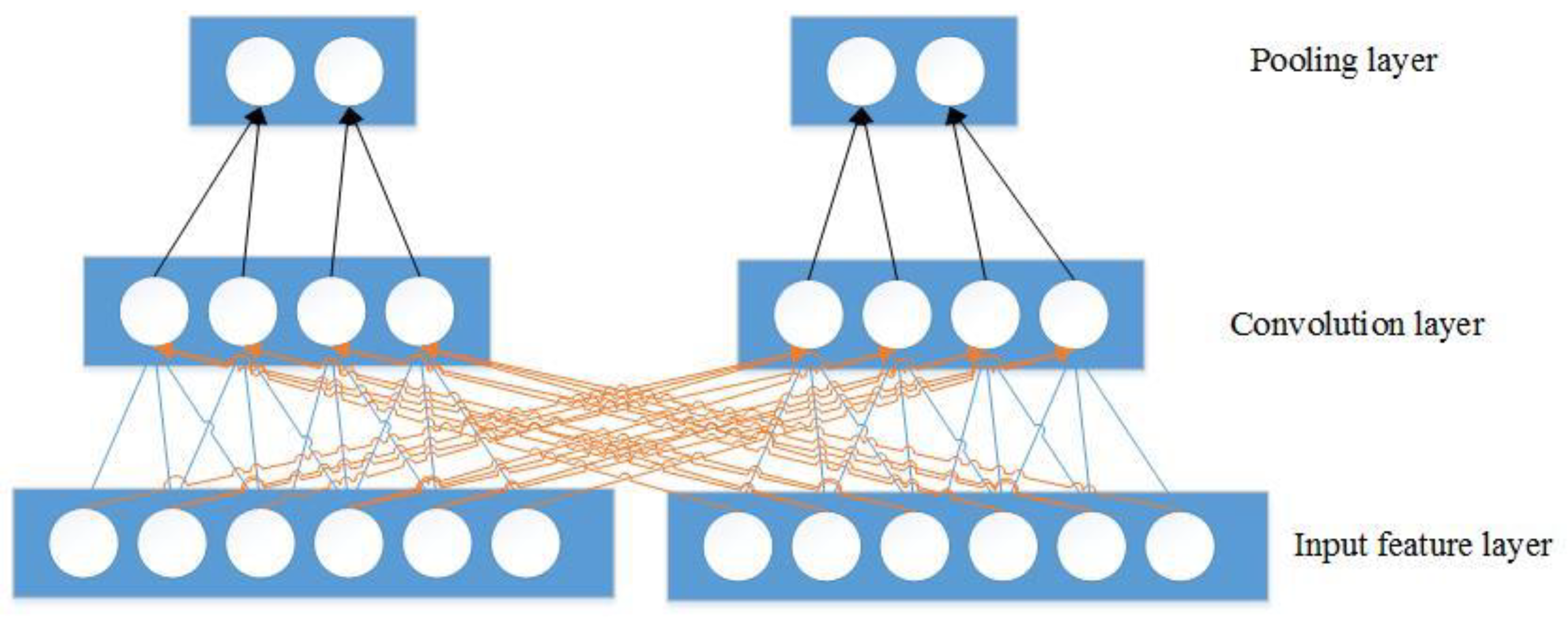
Figure 1. Schematic diagram of the convolution structure.
Energies 13 04900 g001
Figure 2. Long short-term memory (LSTM) hidden layer structure.
Energies 13 04900 g002
Figure 3. Gate recurrent unit (GRU) input and output structure.
Energies 13 04900 g003
Figure 4. Deep learning framework.
Energies 13 04900 g004
Figure 5. Training process of error change. (a)Error comparison of the first epoch; (b) Error of the final epoch.
Energies 13 04900 g005
Figure 6. Average training time of each epoch.
Energies 13 04900 g006
Figure 7. Comparison of each Epoch test error.
Energies 13 04900 g007
Figure 8. Comparison of prediction results.
Energies 13 04900 g008
Figure 9. Error of the five models.
Energies 13 04900 g009
Table 1. Input and output.
Dimension of InputFeature DescriptionDimension of OutputOutput
1time (t) is a time point for every 15 min1From (t) to (t + 3) load
2From (t- time-window) to (t–1) temperature
3From (t- time-window) to (t–1) weather condition
4From (t- time-window) to (t–1) load
Table 2. Weather condition characteristics conversion table.
Weather ConditionMapping ResultsWeather ConditionMapping ResultsWeather ConditionMapping
Results
Overcast0Sand blowing6Heavy rain12
Fog1Heavy snow7Floating dust13
Medium-to-heavy rain2Sunny8Rainstorm14
Light rain3Drizzle9Small-to-medium rain15
Haze4Sleet and snow10Thunderstorms16
Little Snow5Cloudy11Shower17
Table 3. Data display in the first 5 rows of the pre-processed data table.
TimeWeather ConditionTemperatureLoad
2016-01-01 00:00:00 1.738101 −1.394100−0.207188
2016-01-01 00:15:001.738101 −1.410131−0.316169
2016-01-01 00:30:00 1.738101 −1.426163−0.402202
2016-01-01 00:45:001.738101 −1.458227−0.502655
Table 4. Hyperparameters of deep learning model.
Type of HyperparameterExperimental Scene Setting
Number of first layer convolution filters8
Kernel size in Conv Layer 14 × 4
Max pooling size4 × 4
Number of second layer convolution filters16
Kernel size in Conv Layer 23 × 3
LSTM or GRU layer 1; hidden layer unit{20, 50, 80}
LSTM or GRU layer 2; hidden layer unit{20, 50, 80}
Objective functionMSE
Dropout rate0.2
Time step{48, 96, 192}
Batch size{32, 64}
Epoch5
Adam code parameter settings α = 0.001, β 1   = 0.9, β 2 = 0.999
Table 5. List of optimal parameters.
Type of HyperparameterOptimal Experimental Scene Setting
LSTM or GRU layer 1; hidden layer unit50
LSTM or GRU layer 2; hidden layer unit50
Time step288
Batch size32
Table 6. Coefficient of determination.
ModelR2
GRU0.9404
LSTM0.8735
Conv-LSTM0.9705
Conv-GRU0.9191
Conv-GRU-LSTM0.9636