Evaluation of Grid Capacities for Integrating Future E-Mobility and Heat Pumps into Low-Voltage Grids

Abstract

While an area-wide implementation of electric vehicles (EVs) and electric heat pumps (HPs) will contribute to a decarbonization of the energy system, they represent new challenges for existing low-voltage (LV) power grids. Hence, this study investigates potential grid congestions on the basis of three contrasting load approaches applied to four different grid regions. Within the three load approaches, temporal characteristics of various grid customer classes (EVs, HPs, households etc.) are derived from highly resolved realistic load profiles. In accordance with classic grid planning, firstly a static load approach is analyzed by applying the modeled coincidence for each consumer class individually. Secondly, this static approach is modified by including combined coincidence factors, taking temporal consumer class interactions into account. Finally, both static load approaches are compared with detailed annual time series analyses by means of load flow simulations using real-life LV grid data. The evaluation of inadmissible voltage characteristics and thermal congestions identifies future grid extension needs depending on the considered grid region. In addition, the variation of the applied load approach highlights the need to consider consumer-specific temporal behavior. In fact, by neglecting temporal interactions between conventional and future grid customers, the classic grid planning approach overestimates future grid extension needs. To counteract an oversizing of future grid structures, this paper presents a combined consideration of EVs’ and HPs’ coincidence as well as resulting grid consequences on the LV level.

1. Introduction

In 2019, the European Commission announced its vision to achieve the EU’s climate neutrality by 2050 [1]. Considering the energy-related end user greenhouse gas (GHG) emissions in the European Union [2], the transportation and residential sectors represent crucial fields of action. Thus, on the one hand, this vision is further concretized by the European Green Deal [3], which includes, inter alia, a 90% reduction in traffic-related GHG emissions by 2050 as one cornerstone to reach this ambitious goal. Thereby, the EU intends to accelerate the shift to sustainable mobility by an area-wide implementation of one million (2019: 0.14 Mio.) public charging stations by 2025 [3]. In accordance with Norway’s leading role with respect to electric vehicle (EV) numbers [4], this measure will likely result in an increasing number of battery EVs in the EU. On the other hand, the European Commission’s vision is supposed to be realized by increasing the residential sector’s energy efficiency [3], e.g., by an area-wide implementation of electric heat pumps (HPs) [5,6]. In fact, a large-scale transition to electric HPs could decrease the European residential sector’s GHG emissions by up to 30%, assuming a market share of 100% [7]. Besides positive aspects regarding the decarbonization of the traffic and residential sectors, these future technologies will confront the existing power system with new challenges [6]. Since most charging processes take place at home [8,9] and electrical HPs will be installed primarily in residential areas, these challenges will especially affect the low-voltage (LV) level. However, due to today’s relatively low penetration of EVs and electric HPs, these potential consequences for existing distribution grids are hard to identify by the use of actual measurements. Despite the early stage of EV- and HP-penetration, future challenges for distribution system operators (DSOs) have to be analyzed now in order to develop appropriate adaption strategies.

1.1. State of Research

Numerous studies analyze potential impacts of future EVs on the LV level with regards to voltage characteristics [10,11,12,13,14,15], thermal overload of grid lines [15,16], distribution substation (DS) transformer utilizations [12,15,17] as well as the effects on load curves of existing grid customers [11,12,18,19,20,21,22]. Analogously, the implementation of electric HPs and its consequences for existing (LV) grids are investigated by several publications [6,22,23,24,25,26]. Navarro-Espinosa et al. (2016) [27] assess the impacts of, inter alia, EVs and HPs on numerous LV feeders individually based on a Monte Carlo simulation using time series, but their study lacks a combined evaluation of potential synergies. In contrast, the following studies deal with possible grid extension needs induced by an aggregation of these technologies and are therefore described in detail.

Mendaza et al. (2014) [28] use a static Monte Carlo simulation, in order to investigate the capability of a rural LV grid to integrate future EV- and HP-loads. Therefore, the authors vary EVs and HPs spatially in numerous iterations depending on various penetrations, but applying consumer class-specific peak loads exclusively. Hülsmann et al. (2019) [29] analyze the capacity of a German 25,000-noded network to integrate these future grid customers conjunctly considering numerous penetration levels. Based on maximum individual coincidence factors for EVs and HPs, static Monte Carlo simulations are performed. On the other hand, Shao et al. (2013) [30] apply time series with a resolution of one hour in order to examine the integration of a 100% penetration of EVs and HPs into one Danish urban LV grid. Li et al. (2014) [31] analyze EV- and HP-induced voltage deviations and voltage imbalance in one LV feeder based on daily load profiles with a time resolution of one minute, considering several penetration levels. Similarly, Baccino et al. (2014) [32] determine possible grid congestions in one LV grid in order to test the presented demand response algorithms. On this account, they apply daily load profiles considering a certain number of integrated EVs and HPs (one penetration level exclusively). Birk et al. (2018) [33] determine critical voltage characteristics and thermal congestions caused by a penetration of EVs and HPs of 60% in a section of an urban LV grid located in the city center by applying 15-min resolved time series. Finally, Sinha et al. (2020) [34] test the operation flexibility of EVs and HPs combined, implemented into one LV grid. Therefore, one penetration level of these technologies is simulated as the reference scenario, using highly resolved load profiles and a steady-state time series analysis.

In summary, future grid congestions triggered by a combined integration of e-mobility and the electrification of the space heating sector are examined using two different simulation approaches: On the one hand, a static simulation approach considering one time step, mostly in the form of a stochastic Monte Carlo simulation [28,29]. On the other hand, the majority of studies [30,31,32,33,34] apply time series analyses based on time-resolved load profiles. Besides static (stochastic) Monte Carlo simulations, classic power grid planning performed by DSOs is based on an analytical static load approach [35,36] because of its simple and fast application. While Monte Carlo simulations model a variety of grid conditions stochastically based on their probability of occurrence [35], analytical static simulations apply worst-case load conditions. Therefore, the aggregated peak load of a number of grid customers is calculated by multiplying the number of customers by the respective coincidence factor and the average individual peak load [35]. The coincidence factor thereby takes temporal characteristics and resulting load aggregations of numerous grid customers of one consumer class (households, EVs etc.) into account. Both static approaches attempt to consider temporal aggregations for each consumer class individually by the application of individual coincidence factors, whereby temporal interactions between various consumer classes are neglected (e.g., [28,29,35]). Nevertheless, while a stochastic Monte Carlo simulation must be performed for a certain number of iterations [37], any analytical static modeling approach simulating one time step offers advantages in terms of the calculation effort compared to detailed time series analyses [38]. This becomes more important when it comes to the large-scale simulation of numerous grid structures.

Besides the consideration of temporal consumer class interactions, recent studies differ in terms of the analyzed grid region: While the majority fail to define the analyzed grid region (e.g., [29,31,32,34]), urban [30,33] and rural [28] LV grids are investigated in a few studies. However, these studies exclude the fact that real-life housing types (family houses, multi-apartment residential buildings etc.) depend on the considered grid region, which is crucial for evaluating grid impacts especially in urban areas.

1.2. Open Research Questions and Structure of This Paper

The previous section presents the state-of-the-art research in the field of grid simulations analyzing future impacts of EVs and HPs. Thereby, the unanswered research questions with respect to the temporal (1) and spatial (2) components are as follows:

• What impact does the applied load approach have on the estimation of future grid extension needs on the LV level? Is it necessary to take realistic temporal interactions between conventional grid customers, EVs and HPs into account? How can fast static grid simulation meet with a detailed consideration of these consumer class interactions? Does the classic grid planning approach comply with an increase in various grid customer classes, and is it applicable for future grid planning?
• What impact does the considered grid region have on the determination of grid congestions, applying consistent simulation approaches as well as real-life grid topologies and housing types?

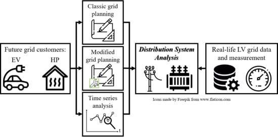
To answer these research questions, this paper identifies potential impacts on the LV level triggered by projected numbers of EVs and HPs based on co-simulations. Therefore, four LV grid structures in various regions are modeled in detail (Section 2.1) using real-life grid data. The method for modeling time-resolved load profiles considering conventional grid customers (Section 2.2.1), future EV charging (Section 2.2.2) as well as future electric HPs (Section 2.2.3) using the software MATLAB [39] is described in this paper. Both grid and consumer load modeling are based on real grid and consumer data, provided in an anonymous form and in compliance with data protection regulations by the Austrian DSO Energienetze Steiermark GmbH [40]. Based on modeled time series, the coincidence of various consumer classes (Section 2.3) is determined depending on the considered number of consumers. To analyze the effects of temporal load aggregations of several grid customers, two static load approaches (applying coincidence factors) as well as a time series-based load approach (Section 2.4) are investigated in the form of load flow simulations using the software NEPLAN [41]. These simulation methods are applied consistently for all LV grids, providing a uniform comparison of various grid regions (Section 3), which are discussed in detail (Section 4).

2. Methodology

2.1. Grid Topologies and Modeling

This analysis deals with the comparison of methods for the determination of potential grid extension needs in various grid regions caused by private charging of EVs and HP loads. Therefore, four real-life LV grids are selected for grid simulations and classified in accordance with the Degree of Urbanization (DEGURBA) defined by the European Commission [42] as urban (densely populated), suburban (intermediate density) and rural (thinly populated). However, we analyze the urban area based on two LV grids, one located in the city center and one located in the city outskirts (

Table 1. Grid configurations depending on the grid region.

	Urban (City Center)	Urban (City Outskirts)	Suburban	Rural
Nom. transformer power [kVA]	2 × 630	630	250	100
No. of feeders	14	12	9	3
No. of PCCs	21	80	87	18
Degree of cabling [%]	100	100	91	57
Admissible building density	0.6–1.2	0.3–0.8	0.2–0.4	0.2–0.3
Total line length [km]	2.17	6.13	5.64	2.31
Share of family houses [%]	0	87.5	100	100

). The selected LV grids are each characterized by a DS (Figure 1), transforming the medium voltage (MV) of 20 kV to a nominal voltage of 400 V (phase-to-phase) via a three-phase transformer (vector group Dyn5). With a classic radial grid structure typical for the LV level [43], this substation supplies a number of feeders and points of common coupling (PCCs) via cables or overhead lines. However, the suburban and urban grids are equipped with several grid separation points, enabling the creation of a partial ring network structure in case of failure. The selected LV grids show significant differences (Table 1) in terms of nominal transformer power at the DS, number of feeders, number of PCCs, degree of cabling, admissible building density, total line length and the share of family houses (FHs).

The latter is especially significant for the possibility of investigating private parking at home or the installation of electric HPs. While FHs are predominant in the suburban and rural area, the urban grid located in the city center is characterized by multi-apartment residential buildings (MARBs) exclusively, which show limited possibility for private parking and inhibit the installation of HPs. For the implementation of load flow simulations, the mentioned grid configurations (e.g., Figure 1) are modeled in detail using the software NEPLAN [41]. For this purpose, real-life line- and transformer-specifications as well as real-life PCC-allocations of present grid customers are applied. As a result, potential grid consequences (e.g., voltage deviations and thermal overload) are identified with a high level of detail. In each of the four grid models, the higher voltage side of the DS is connected to a slack node (Figure 1), providing constant voltage. Consequently, voltage deviations in the MV level are excluded, which is taken into account when contrasting node voltages with standardized voltage limits (e.g., Section 2.4.2).

To model future grid customers, each PCC is equipped with six load modules, representing conventional consumer loads—present household (HO) loads, commercial businesses (CBs), agricultural businesses (ABs), electrical water heaters (WHs)—future EV charging loads (EV) as well as future electric HP demands (HP). All of these load modules are provided with either static load values or annual time series with a time resolution of one minute in order to perform long-term load flow simulations.

2.2. Modeling of Grid Loads as Time Series

2.2.1. Conventional Consumer Loads

Spatially and time-resolved loads of conventional grid customers are modeled separately depending on their consumer class. Therefore, consumers are classified in accordance with Austrian Grid Codes [44] into HOs as well as CBs, ABs and WHs (

Table 2. Number of persons (estimated) and number of conventional grid customers depending on consumer type and grid region.

	Urban (City Center)	Urban (City Outskirts)	Suburban	Rural
Estimated number of persons	509	346	231	50
Households (HOs)	331	170	88	18
Commercial businesses (CBs)	76	31	22	1
Agricultural businesses (ABs)	0	1	10	4
Electrical water heaters (WHs)	298	85	19	2

). In the first step, time series of CB-, AB- and WH-loads are modeled by means of standardized load profiles pursuant to [45], which further classifies them into seven CB types, three AB types and six WH types.

These load profiles provide annual phase-balanced active power time series for numerous consumer classes unified for an annual energy consumption of 1000 kWh. Finally, the scale of these unified load profiles by the real consumer’s annual energy demand provides consumer class-dependent active and reactive power loads (a power factor of 0.98 lagging is assumed). Besides these standardized load profiles, HO load profiles are modeled with the behavior-based load profile generator by Pflugradt [46]. Thereby, this tool provides pre-defined HO structures, which differ in terms of the number, age and behavior of residents. For each of the grid’s HOs, one of these pre-defined HO structures and its according active load profile is selected randomly based on the number of persons. While the number of persons of pre-defined HO structures is provided by the applied load profile generator, this information is not available within the DSO’s data. Therefore, the number of persons is estimated for each of the LV grids’ HOs by the real-time annual energy consumption and an average energy demand of 2050 kWh per person [47]. This results in an aggregated number of 509 (urban—city center), 346 (urban—city outskirts), 231 (suburban) and 50 (rural) persons (Table 2). After selecting the appropriate pre-defined HO (active power) profile based on the estimated number of persons, reactive power characteristics are taken into account depending on households’ underlying devices and their power factor [48,49]. All the modeled time series cover one year with a time resolution of one minute, taking seasonal as well as daily load deviations into account. Finally, all types of conventional consumer loads (CB-, AB- and WH-loads as well as HO-loads) are aggregated for each PCC (e.g., Figure 2), distributed symmetrically to all the grid phases and calibrated with real data acquired by long-term measurements (described in detail in Appendix A.1). The load profile calibration using measured data enables an (almost) exact load simulation on the DS level considering conventional grid customers exclusively (neither EV nor HP). Nevertheless, since measured transformer loads at the DS level include grid losses during operation, this calibration results in a slight overestimation of conventional consumer loads. As a result, the maximum thermal utilization of the LV grids’ transformers determined by grid simulations in the form of time series analyses exceeds the measured one by 0.57% (urban: city center), 0.55% (urban: city outskirts), 0.64% (suburban) and 2.02% (rural). Still, the performed load profile calibration allows for an accurate consideration of existing grid customers, required for a detailed analysis of the LV grids’ capacity for integrating additional consumer loads, such as EVs or HPs.

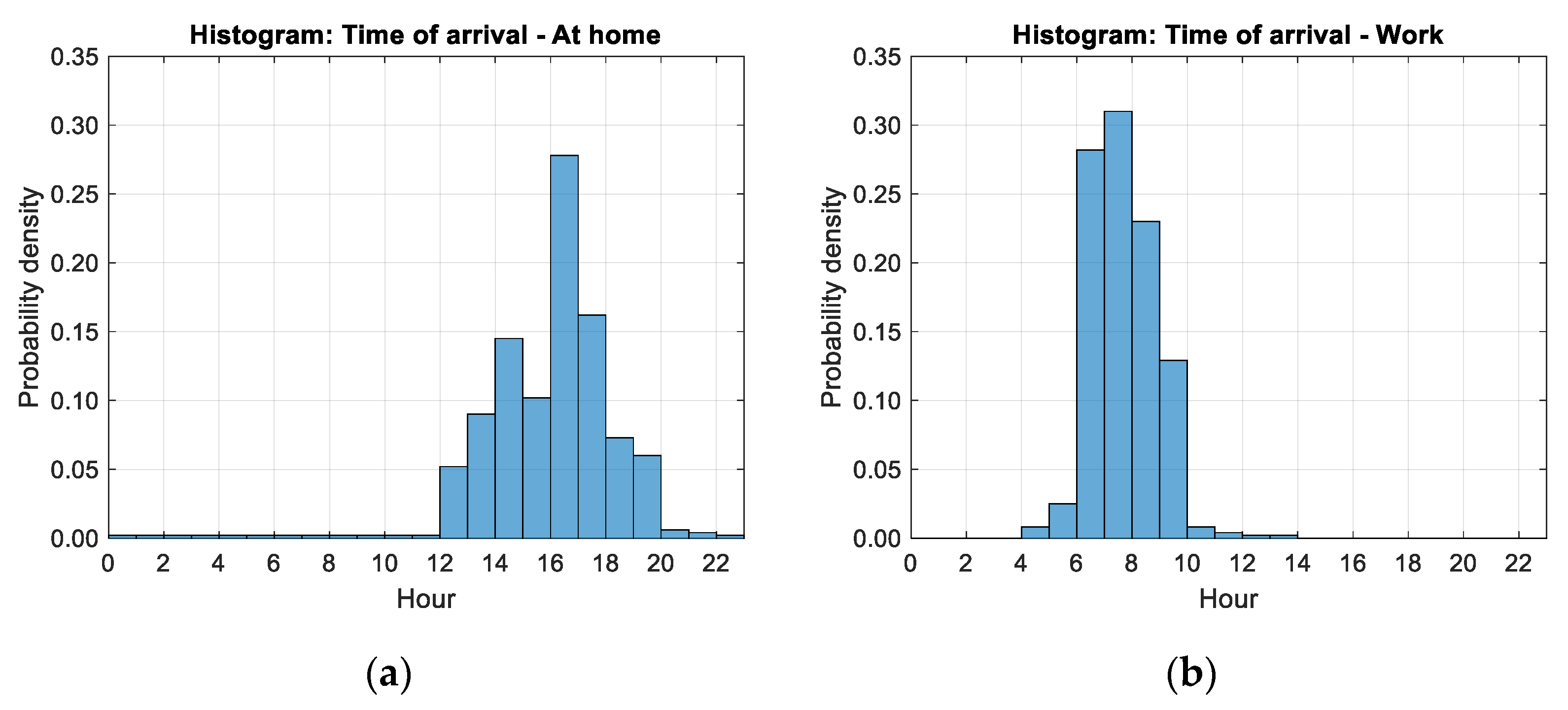
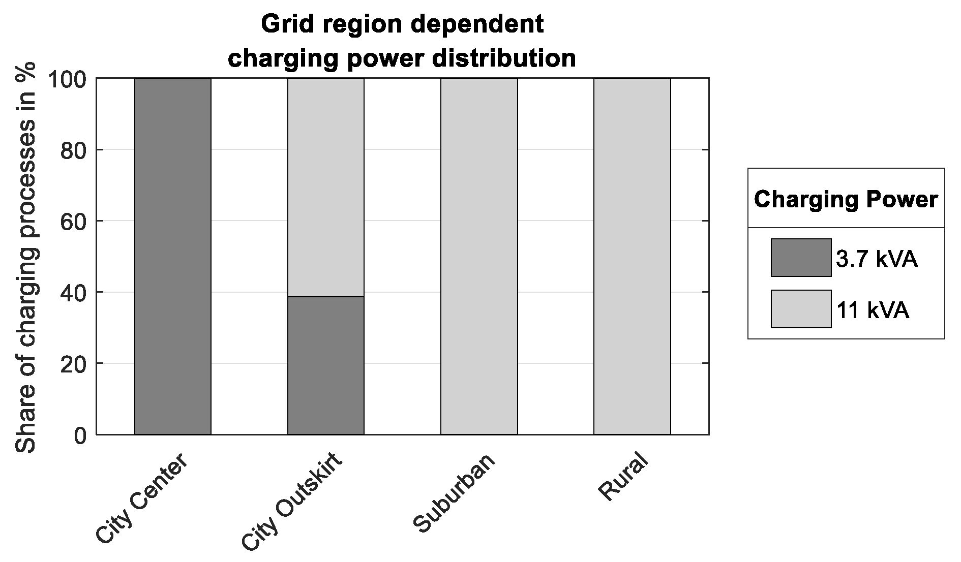
2.2.2. Electric Vehicle Charging Loads

In addition to conventional grid customers, this study deals with potential grid impacts caused, inter alia, by the future supply of EVs, charged at private charging points. The European Directive 2014/94/EU of the European Parliament and of the Council of 22 October 2014 on the deployment of alternative fuels infrastructure [50] defines public charging infrastructure for EVs as non-discriminatory access for all users within the European Union. However, due to a missing definition of private charging, all charging possibilities may be defined as private charging points, which violates non-discriminatory access, e.g., by several kinds of authorization, usage or payment. Hence, two of these private charging EV user groups are taken into account in this study:

• Charging at home: This user group deals with EVs charged at domestic charging points
• Charging at work: EVs of this user group are charged at the enterprise parking area

Analogously to the methods applied in previous studies [12,51,52], an uncontrolled, stochastic charging behavior is taken into account for both of them. To model this stochastic charging behavior, the following aspects must be considered individually for each user group: the spatial distribution of charging points, individual mobility patterns (time of charging and covered distance), EV model specifics (battery capacity, specific energy consumption, charging efficiency and charging power). A detailed description of the stochastic determination of these characteristics is presented in Appendix A.2, Appendix A.3, Appendix A.4 as well as in the authors’ recent publications [53,54,55].

Before modeling time series of EV charging loads, the actual charging power must be defined for each connection between an EV and its charging point. Therefore, the available installed power of private charging infrastructure depending on the grid area must be taken into account: Private parking or rather charging possibilities depend significantly on the housing type, which is differentiated into FHs and MARBs. In Austria (and a few other countries), the vast majority of HOs are integrated into the LV level based on a three-phase connection [36], tolerating a maximum installed charging power of 11 kVA. Nevertheless, most of the charging points in MARBs are equipped with reduced charging power [56]. Hence, charging points at FHs and at work are in this study considered to be equipped with 11 kVA available power, whereas charging points at MARBs are considered to provide only limited power of 3.7 kVA per charging point. Since all of the considered EV models enable charging with 11 kVA (Appendix A.4), the actual available charging power depends solely on whether it is charged at a FH, a MARB or at work. As a result, EVs are charged with 11 kVA in the rural (100% of charging processes), the suburban (100%) and the urban LV grid located in the city outskirts (61.3%). In contrast, 100% (city center) and 38.7% (city outskirts) of charging processes are supplied with 3.7 kVA by the urban LV grids (Figure 3). Assuming a uniform phase-allocation at MARBs, low-power charging with 3.7 kVA (usually in the form of single-phase charging) is considered as phase-balanced three-phase charging.

Finally, after determining the spatial distribution of private charging points (where are EVs charged?), user group-specific mobility patterns, state-of-the-art EV model specifics (when and for how long are they charged?) and the available charging power (with which power?), annual time series of EV charging loads with a time resolution of one minute are modeled for each EV. Therefore, measured charging data available for all the listed EV models (

Table A5. Specifics of EV models applied for modeling EV charging loads.

EV Model	Frequency (%) [68]	Battery Capacity (kWh) [69]	Specific Energy Consumption (kWh/km) [69]	Charging Efficiency (-) 1 [69]
1	19.0	41	0.203	0.828
2	16.8	75	0.209	0.838
3	15.0	27.2	0.184	0.708
4	8.6	34.9	0.173	1.000
5	7.3	17.6	0.183	1.000
6	6.4	95	0.237	1.000
7	6.3	64	0.195	0.866
8	4.5	40	0.221	1.000
9	4.1	17.6	0.183	1.000
10	3.2	28	0.147	0.906
11	2.9	27	0.191	1.000
12	1.6	90	0.276	0.893
13	1.5	90	0.240	1.000
14	1.3	18.7	0.177	1.000
15	1.3	40	0.281	0.853

¹ In the case of an efficiency of 1.0, charging losses are included in the energy consumption.

), including phase-imbalanced active and reactive power profiles, are applied. Depending on the selected EV model (Appendix A.4), the measured charging data are scaled according to the defined charging power, while maintaining original (measured) power factors. For each charging event, these scaled charging curves are adapted pursuant to the required amount of energy and added to the EV-specific annual load profile according to the time of charging. After modeling EV charging load profiles (one year) for all EVs, active and reactive power profiles are aggregated for each PCC (e.g., Figure 2), in accordance with the EVs’ spatial allocation depending on the considered EV-penetration.

2.2.3. Electric Heat Pump Loads

Analogous to the modeling of time-resolved EV charging loads, potential grid impacts triggered by electric HPs depend on a spatial (where?) and a temporal (when?) component. For dealing with the former, the same approach as for determining the spatial distribution of private EV charging points (Appendix A.2) is applied. Therefore, the maximum number of HPs (HP-penetration of 100%) within each LV grid is initially detected based on the respective housing type (FH or MARB). Since only FHs allow the installation of future HPs, the maximum number of potential HPs equals the number of FHs supplied by the according LV grid: 0 (urban—city center), 60 (urban—city outskirts), 70 (suburban) and 15 (rural). Similar to the analysis of future EV numbers, this study analyzes potential impacts induced by future HP-penetrations (0%, 5%, 10%, 20%, 30%, 50% and 80%). However, for defining which FH is virtually equipped with a HP considering a certain HP-penetration, a uniform HP-share is applied to each of the LV grid’s feeders.

For modeling the temporal component on the other hand, time-resolved HP load profiles, pre-defined for numerous house structures (e.g., single-family house hosting 1–2 persons, house with a solar thermal system, 300 L storage tank and gas heating etc.) are acquired also by Pflugradt [46]. Furthermore, these HP load profiles are uniformly scaled according to an average domestic space heating demand of 14,316 kWh/a/household and an average domestic warm water demand of 2995 kWh/a/household [57,58] assuming a coefficient of performance of 3.0. Reactive power profiles are derived by applying a constant power factor of 0.9 (lagging) [23,24,26]. Finally, considering a certain HP-penetration, the individual HP-loads of FHs are aggregated for the supplying PCC (e.g., Figure 2) in accordance with the spatial determination, defined in the previous step. The modeled HP load profiles show HP-typical characteristics according to Brendan et al. (2014) [23], e.g., increased starting current/power due to the compressor motor as well as a certain base load during operation. If an FH is virtually equipped with a HP, the previously modeled electric water heating loads (WH) as well as loads for electrical space heating are neglected.

2.3. Modeling the Coincidence of Current and Future Grid Loads

The coincidence of grid customers’ electrical loads represents a crucial aspect for grid operators regarding the planning and operation of power grids. This “is a measure of the simultaneity of peak demands of a group of N customers” [35] and describes temporal aggregations of numerous electric loads: Considering a certain number of grid customers, a high coincidence equals a high probability for a power demand at the same time. Equation (1) [35] describes this correlation in the form of the coincidence factor (CF) considering a certain number of customers (NoC). It is defined by the ratio between the maximum of the aggregated load, $\max \left({\displaystyle \sum }_{i=1}^{NoC}{P}_i\left(t\right)\right)$, and the aggregated maxima of individual loads, ${\displaystyle \sum }_{i=1}^{NoC}\max \left(P_i\left(t\right)\right)$.

$$CF\left(NoC\right)=\frac{\max \left({{\displaystyle \sum }}_{i=1}^{NoC}{P}_i\left(t\right)\right)}{{{\displaystyle \sum }}_{i=1}^{NoC}\max \left(P_i\left(t\right)\right)}$$

(1)

Due to currently low EV- and HP-penetrations, real information with respect to the coincidence of numerous charging EVs and HPs is missing. On account of this, the presented analysis provides the coincidence of existing and future grid customers based on long-term time series with a resolution of one minute, necessary for deriving the exact coincidence of grid customers [35]. Therefore, the modeled load profiles of households (HOs), commercial businesses (CBs), agricultural businesses (ABs), electrical water heaters (WHs), electric vehicles (EVs) and electrical heat pumps (HPs) are applied for each grid respectively. Since this study investigates potential grid impacts within a time period of one year, the maximum coincidence is stochastically modeled for this period and each NoC. Assuming an NoC of ten units for example, ten daily load profiles of the according consumer class are randomly selected, aggregated and divided by the aggregated maxima of these selected load profiles for each day of the year, according to Equation (1). Finally, the year’s maximum CF (maximum of 365 daily values) is detected for each NoC and each consumer class, demonstrated in Figure 4a for the suburban LV grid.

In addition to varying consumer classes, two different approaches for dealing with the coincidence between these are investigated by this study: the CF-modeling for each consumer class individually (Figure 4a) as well as the CF-consideration of various consumer classes combined (Figure 4b). The former determines the coincidence of each consumer class on its own, neglecting the temporal correlation with other consumer classes (e.g., as applied in [29] using a Monte Carlo simulation). In contrast, the latter takes temporal interactions between various consumer classes into account by aggregating all kinds of electrical loads supplied by the power grid. Based on numerous possible customer class compositions, the combined coincidence at a certain aggregated NoC varies within the modeled and illustrated bandwidth (Figure 4b). In addition, Figure 4b highlights CF-areas defined by a predominant proportion (>75%) of HOs, EVs or HPs in relation to the total aggregated NoC. As already demonstrated by an individual CF-consideration (Figure 4a), EVs are characterized by increased simultaneity compared to HOs and HPs. Consequently, the analysis of grid customers representing EVs primarily requires a higher CF compared to customer groups with a predominant share of HOs or HPs, especially at a low aggregated NoC. Based on the assumed uncontrolled charging primarily during evening hours (Appendix A.3), a CF of (almost) one is determined even at a number of four vehicles (Figure 4a), considering EV charging with 3.7–11 kVA and both EV user groups. Regardless of consumer class and modeling approach, the probability of a simultaneous grid demand and thereby the CF decreases with an increasing number of customers [35] starting from one. The application of standardized load profiles for modeling CBs, ABs and electric WHs (Section 2.2.1) results in high coincidence compared to other consumer classes. In fact, a more accurate modeling of their coincidence would require more individual load profiles, e.g., measured during real-life operation.

2.4. Grid Simulations Using Load Flow Calculations

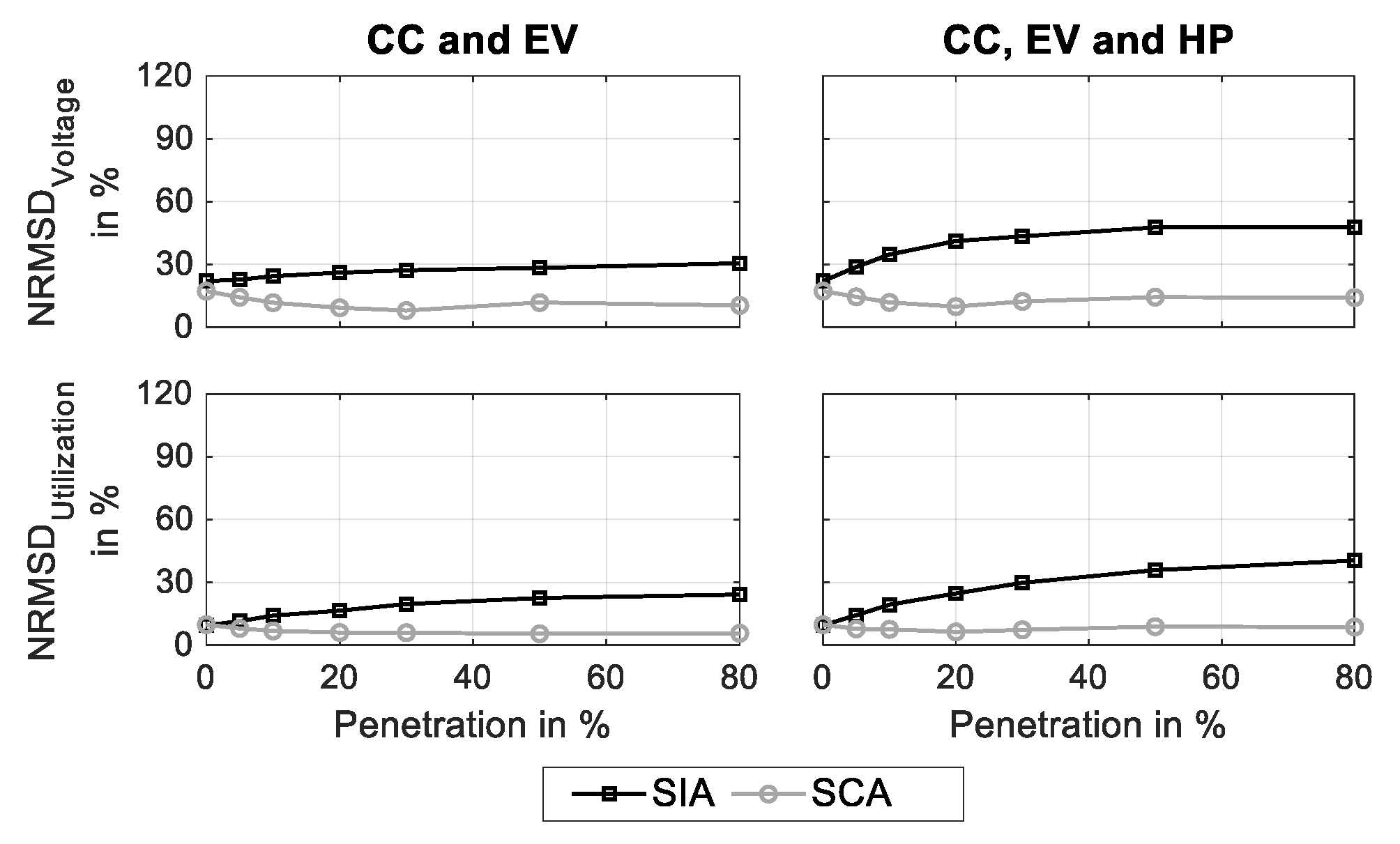
2.4.1. Load Approaches Analyzing Temporal Interactions between Various Consumer Classes

In this study, we analyze two static simulation approaches based on the modeled coincidence (Figure 4) in combination with the aggregated peak power of modeled load profiles. On the one hand, we investigate a static individual aggregation (SIA) of several consumer classes in accordance with classic grid planning [35], using the consumer class-individual coincidence factors. Hence, the electrical grid customers’ aggregated load $P$ in this approach is calculated by accumulating the mathematical product of the maximum power of each consumer class $P_{max, class}$ and the according individual coincidence factor $C{F}_{ind, class}$ for all the considered consumer classes (

Table 3. Comparison of various load approaches applied for grid simulation.

Load Approach	No. of Time Steps	Power Determination
Static individual aggregation (SIA)	1	$P={\displaystyle {\displaystyle \sum }_{class=1}^{No.of classes}}\left(P_{max, class}·C{F}_{ind, class}\right)$
Static combined aggregation (SCA)	1	$P=\left({\displaystyle {\displaystyle \sum }_{class=1}^{No.of classes}}{P}_{max,class}\right)·C{F}_{comb, No.of classes}$
Time series analysis (TSA)	525,600	$P=\underset{}{\max \left({\displaystyle {\displaystyle \sum }_{class=1}^{No.of classes}}{P}_{class}\left(t\right)\right)}$

).

On the other hand, a static combined aggregation (SCA) of various consumer classes is examined within a second approach: The electrical grid customers’ aggregated load $P$ results from the aggregation of the maximum power of each consumer class $P_{max, class}$ multiplied by a consumer class-combined coincidence factor $C{F}_{comb, No.of classes}$. The latter is selected from the modeled CF-bandwidth (Figure 4b) depending on the number of HOs, CBs, ABs, WHs, EVs and HPs. The maximum power of each consumer class $P_{max, class}$ is defined by the maximum of the aggregated load profile, including a certain number of consumers of a certain consumer class (e.g., ten households).

Despite similarities between these two static simulation approaches (SIA and SCA), they differ significantly with regards to the consideration of temporal overlaps between considered electrical consumer classes. This difference is demonstrated by a simple load determination, considering 32 HOs (with a peak load of 2 kVA each), three CBs (3 kVA each), seven ABs (2 kVA), three electric WHs (5 kVA), 45 EVs (11 kVA) and 21 electrical HPs (10 kVA), resulting in an aggregated peak load of 807 kVA. The SIA applying individual coincidence factors of 0.195, 0.96, 0.756, 0.973, 0.339 and 0.262 (Figure 4a) results in an aggregated peak load of 269.1 kVA. In contrast, a combined consideration of grid customers’ coincidence (SCA) of 0.181 (highlighted in Figure 4b) results in an aggregated peak load of 146.1 kVA (−46%). In addition to these static load approaches, a real-life simulation approach on the basis of modeled annual time series with a time resolution of one minute is applied. Using this time series analysis (TSA), the electrical grid customers’ aggregated load $P$ is identified by the maximum of aggregated load profiles including all consumer classes (Table 3). While the TSA enables the implementation of time-resolved reactive power profiles (Section 2.2), constant power factors (PF) are applied in order to determine the reactive power demand in the SIA- and SCA-approach. Therefore, an average PF of 0.955 (lagging) is estimated considering existing grid loads based on long-term measurements at the DS (Figure A1) and applied for consumer classes HO, CB, AB and WH. Similarly, the reactive power demand of EVs is determined by measured charging data (applied for modeling time series of EV charging loads) including 15 varying EV models. These measured charging data demonstrate, that for most EV models, the power factor strongly differs between constant-current-phase (average PF of 0.995, leading) and constant-voltage-phase (0.280, leading) during the charging process. Consequently, an annual average PF including all the modeled time series of EV charging is detected (0.971, leading) and applied for the SIA- and SCA-approach. Due to missing measurement data regarding electrical HPs, a PF of 0.9 (lagging) [23,24,26] is assessed, analogous to the modeled time series (Section 2.2.3). For a combined aggregation of various consumer classes in the SCA-approach, an average PF weighted by individual numbers of consumer classes is applied in a simplified manner (e.g., the combined consideration of two HOs, two EVs and one HP results in a PF of 0.993, lagging).

2.4.2. Evaluation of Grid Reinforcement Needs

To examine the future need for grid extensions in various LV grids, induced by EVs and/or HPs, the mentioned load approaches are analyzed by determining grid loads at certain grid locations (Figure 5) including the DS and each feeder separately. Therefore, both static load approaches require the number of grid customers (for identifying the according CF) and the aggregated peak load of each consumer class, depending on the considered point of load determination. The aggregated load calculated at these locations is distributed to all involved PCCs (points of load application in Figure 5) according to their contribution to the feeders’ or distribution substation’s peak load. In the TSA-approach, time series are modeled for each of the involved grid customers and aggregated for each time step in accordance with the point of load application. To evaluate inadmissible voltage characteristics caused by future EV- and HP-numbers, voltage deviations are detected at the distribution substation’s LV side (DS1; Figure 5) as well as at the farthest grid node in each feeder (e.g., F1; Figure 5). Furthermore, detected voltage deviations are examined regarding the compliance with EN 50,160 [59], which defines an admissible voltage range of ±0.1 per unit (pu) compared to the nominal voltage. In fact, this permitted voltage range is shared by the MV and LV levels conjunctly. However, pursuant to the voltage range partitioning presented in [60], a voltage range of only [−0.065 pu; +0.045 pu] is available on the LV level.

As a result, this admissible voltage range is taken into account to evaluate the number of critical grid nodes with respect to inadmissible voltage deviations. Besides voltage characteristics, potential needs for grid reinforcement measures are additionally derived based on the thermal utilization of feeders (e.g., F1; Figure 5) and the thermal utilization of the distribution substation’s transformer (DS1).

3. Results

This study deals with potential grid impacts caused by future grid customers by analyzing three varying load approaches and four different grid regions. Therefore, the results of performed grid simulations in the form of load flow calculations are classified accordingly: Firstly, deviating results in terms of voltage characteristics and thermal overload considering the analyzed load approaches are presented (Section 3.1). Secondly, this study provides an estimation of future grid expansion needs depending on the grid region, the applied load approach and the considered EV- and HP-penetration (Section 3.2).

3.1. Comparison of Various Load Approaches

To demonstrate the influence of the applied load approach, voltage deviations (Figure 6) and thermal utilizations (Figure 7) are contrasted considering the LV grids’ distribution substation (DS1) and feeders (F1, F2 etc.). Due to the fact that it has the highest number of EVs and HPs, the load approach comparison is demonstrated using the suburban LV grid’s simulation results. Therefore, three degrees of existing and future grid customers are investigated taking various EV- and HP-penetration levels into account: conventional consumers only (CC), conventional consumers in combination with EVs (CC and EV) as well as conventional consumers in combination with EVs and HPs (CC, EV and HP). The evaluated voltage deviations in the suburban LV grid (Figure 6) considering these different degrees of consumer classes differ significantly with the applied load approach. The SIA-approach results in minimal voltages (feeder F4) of 0.955 pu (CC), 0.933 pu (CC and EV) and 0.915 pu (CC, EV and HP), exceeding the defined voltage limit of 0.935 pu even at an EV-penetration of 5%. Additionally, a voltage decrease of 0.017 pu (CC), 0.018 pu (CC and EV) and 0.022 pu (CC, EV and HP) is detected at the LV side of the distribution substation (DS1). As a result, one (CC and EV) or rather three feeders (CC, EV and HP) face inadmissible voltage reductions caused by charging EVs or rather EVs in combination with HPs.

In contrast, the SCA- and TSA-approaches show rather similar impacts on voltage deviations, all complying with the admissible voltage range: While conventional consumers only (CC) causes a minimal voltage (F4) of 0.964 pu (SCA) and 0.968 pu (TSA), these values decrease to 0.961 pu (SCA) and 0.954 pu (TSA) supplying 5% EVs or rather to 0.951 pu (SCA) and 0.948 pu (TSA) supplying 5% EVs and HPs (Figure 6). Using the SCA-approach, the following voltages are detected at DS1: 0.989 pu (CC), 0.988 pu (CC and EV) and 0.988 pu (CC, EV and HP).

Otherwise, voltages of 0.992 pu, 0.991 pu and 0.990 pu are triggered at DS1 by these grid loads applying the TSA load approach. In addition to CC-, EV- and HP-caused voltage deviations, we discover a maximal thermal utilization in the LV grid’s most critical feeder (F4) of 40.4% (CC), 61.3% (CC and EV) and 73.0% (CC, EV and HP) presuming the SIA-approach. The SCA load approach on the other hand results in a thermal load of 36.3%, 38.2% and 50.4%. Finally, a maximal thermal utilization of 29.4%, 38.2% and 41.4% is determined based on the TSA-approach (Figure 7).

Analogously, the evaluation of the suburban LV grid’s transformer (DS1) illustrates a similar trend: 74.7% (CC), 97.3% (CC and EV) and 114.1% (CC, EV and HP) are detected using the SIA-approach; 48.9%, 56.5% and 57.1% using the SCA-approach; and 41.9% (CC), 57.2% (CC and EV) and 59.1% (CC, EV and HP) using the TSA-approach. Besides differences regarding the most critical grid locations—e.g., feeder F4 (voltage) and the transformer at the DS (thermal overload)—we analyze the correlation between load approach-induced deviations and the number of additional grid customers in the grid. Therefore, we determine the normalized root mean square deviation (NRMSD) between the static load approaches (SIA and SCA) and the time series analysis (TSA) as a function of numerous EV- and HP-penetration levels: Equations (2) and (3) show the NRMSD’s exact calculation regarding voltage $V$ deviations (referring to an admissible voltage range of 6.5 pu) and thermal utilization $U$ deviations (referring to a maximal thermal load of 100%) including all feeders.

$$NRMS{D}_{Voltage}=\frac{\sqrt{\frac{1}{No. of feeders}·{{\displaystyle \sum }}_{i=1}^{No. of feeders}{\left(V_{TSA}-V_{SIA or SCA}\right)}^2}}{Admissible voltage range of 6.5 pu}$$

(2)

$$NRMS{D}_{Utilization}=\frac{\sqrt{\frac{1}{No. of feeders}·{{\displaystyle \sum }}_{i=1}^{No. of feeders}{\left(U_{TSA}-U_{SIA or SCA}\right)}^2}}{Admissible maximal thermal load of 100\%}$$

(3)

Figure 8 demonstrates load approach-induced NRMSDs compared to the TSA for the suburban LV grid depending on the considered EV- and HP-penetration. The NRMSD analysis for the urban LV grid in the city center (Figure A5), the urban grid in the city outskirts (Figure A6) as well as the rural LV grid (Figure A7) is demonstrated in Appendix A.5. It points out that the static load approaches differ when it comes to the grid simulation of numerous different grid customer classes and penetration levels: Considering the supply of conventional consumers (CC)—HOs, CBs, ABs and electrical WHs—only (EV- and HP-penetration of 0%), the estimation using the SIA-approach deviates by 19.64% (voltage) and 12.12% (utilization) from the according thresholds (6.5 pu and 100%) compared to the time series analysis (Figure 8). In contrast, the application of the SCA load approach results in an NRMSD of 7.93% and 3.93%.

Both voltage- and utilization-NRMSD show very similar trajectories as a function of increasing EV- and HP-penetrations. Nevertheless, they differ significantly depending on the applied load approach. On the one hand, the SCA- and TSA-approaches provide very similar results rather independent of the EV- and HP-penetration (Figure 8): The determined NRMSD_Voltage fluctuates between 4.62% (5% EV- and HP-penetration) and 24.62% (80% EV-penetration), and the NRMSD_Utilization fluctuates between 1.98% (5% EV-penetration) and 12.77% (80% EV- and HP-penetration). On the other hand, the NRMSD between the SIA- and the TSA-approach increases decisively when considering an additional customer class: While the simulation of conventional grid customers in combination with future EVs (CC and EV) results in maximal NRMSD_Voltage and NRMSD_Utilization of 30.77% (20% EV-penetration) and 23.72% (80%), these values increase to 86.15% and 59.44% (both at 80% EV- and HP-penetration) when including additional HPs (CC, EV and HP).

3.2. Comparison of Different Grid Regions

In addition to the load approach analysis, we analyze future grid extension needs in four different grid regions. Therefore, the share of critical feeders with respect to inadmissible voltage characteristics (dropping below 0.935 pu) and thermal overloads (exceeding 100%) is determined for each LV grid and each load approach (Figure 9 and Figure 10), considering CC and EVs (a) as well as CC, EVs and HPs (b). The evaluation of inadmissible voltage deviations shows a clear influence of the considered grid region in particular. The urban LV grid located in the city center shows no impacts on voltage characteristics, neither with regard to the applied load approach nor with regard to the degree of grid customer classes (Figure 9). The urban grid located in the city outskirts faces critical voltage decreases starting with 10% (SIA), 80% (SCA) and 30% (TSA) EV- and HP-penetration. Still, the supply of conventional consumers in combination with EVs (without HPs) can be provided even for high EV numbers (Figure 9b), applying the SCA or TSA. Using the SIA, this provision is limited to an EV-penetration of 10% in 8.3% (one) of all feeders. Initial voltage problems also occur even at low penetration levels in at least one of the suburban grid’s feeders: 5% (SIA) and 30% (SCA and TSA) penetration supplying CC and EV and 5% (SIA), 30% (SCA) and 20% (TSA) integrating additional HP-loads (Figure 9). Similarly, the rural LV grid is strongly affected by future EV- and HP-numbers with respect to critical voltage deviations. While only 10% (SIA and TSA) and 20% (SCA) of EVs can be supplied, the integration of additional HPs is restricted to 10% (SCA and TSA) or even impeded completely (SIA).

Furthermore, the SIA-approach determines thermal overloads caused by CC and EVs in at least one feeder in the urban grid located in the city outskirts (80% EV-penetration) and the suburban one (50%). The supply of CC, EVs and HPs on the other hand triggers grid line overloads at 30% (outskirts), 20% (suburban) and 80% (rural) EV- and HP-penetration (Figure 10). Using the SCA- or TSA-approach, thermal problems only occur in one feeder in the suburban LV grid at 80% (CC and EV) and 50% (CC, EV and HP) penetration.

In addition to critical voltage characteristics and thermal overloads, we investigate the maximal thermal utilization of the LV grids’ DS depending on the supplied grid customers (Figure 11): CC and EV (a) or CC, EV and HP (b). The urban (city center) grid’s transformer shows a maximal thermal load of 75.8% (SIA), 46.1% (SCA) and 28.2% (TSA) supplying CC and EV and thereby the compliance with its nominal transformer capacity (Table 1). Since the investigated urban grid structure impedes the installation of HPs, no additional loads are added in the CC, EV and HP scenario.

The urban grid located in the city outskirts faces grid restrictions (only) when applying the static individual load aggregation (SIA) and considering CC, EV and HP. In fact, the supply of these EV- and HP-numbers results in a maximal transformer load of 114.80% (SIA), 66.44% (SCA) and 71.91% (TSA). Without integrated HPs, the maximal transformer load decreases to 94.6% (SIA), 55.8% (SCA) and 58.1% (TSA). In the suburban LV grid on the other hand, the congestion of the transformer’s capacity depends strongly on the applied load approach: While the SIA-approach results in a maximal thermal utilization of 106.0% (CC and EV) and 130.8% (CC, EV and HP) powering a penetration of 10%, the SCA- (66.5% and 72.8%) and TSA-approach (66.8% and 69.7%) estimate this scenario differently (Figure 11). An integration of numerous EVs (80% penetration) creates a maximal thermal utilization of 225.1% (SIA), 179.5% (SCA) and 172.4% (TSA) in the suburban grid’s DS, whereas the installation of additional electric HPs increases this load to 298.9%, 187.7% and 211.9%. Despite lower nominal capacity (Table 1), the rural grid’s transformer shows quite similar results in this respect (Figure 11): Initial thermal restrictions are triggered by 20% (CC and EV) and 10% (CC, EV and HP) applying the static individual load aggregation (SIA). Using the static combined load approach (SCA), these EV- and HP-numbers induce a maximal thermal utilization of 71.7% and 80.7%. Furthermore, the performed time series analyses (TSAs) indicate utilizations of 74.3% (CC and EV) and 82.0% (CC, EV and HP) compared to the nominal transformer power.

4. Discussion

By means of static (SIA and SCA) and time series-based (TSA) load flow calculations, we analyze the impacts of the following factors on the identification of future grid extension needs on the LV level:

• The consideration of temporal load aggregations of various grid consumer classes in the form of three load approaches;
• The investigated grid region, including realistic housing types, affecting the available charging power and HP-numbers.

The analyzed load approaches—static individual aggregation (SIA), static combined aggregation (SCA) and time series analysis (TSA)—vary in terms of the consideration of temporal interactions between numerous consumer classes: While the SIA-approach assumes a temporal aggregation of all consumer classes’ peaks, the other two take consumer class-specific peak periods into account, either by “combined” coincidence factors (SCA) or stochastically modeled time series (TSA). On both the DS-transformer level as well as the feeder level, grid analyses based on the static load aggregation applying an individual coincidence (SIA) result in an overestimation of aggregated maximal loads, compared to the SCA- and TSA-approach. Neglecting temporal consumer class interactions, peak loads of all consumer classes are summed up, resulting in increased voltage decreases (Figure 6) and thermal utilizations (Figure 7). As a result, even the simulation of existing grid customers only (0% penetration) in the form of HOs, CBs, ABs and WHs reveals much higher transformer load (e.g., 74.7% in the suburban grid) compared to that measured during real-life operation (42.0%). This high degree of deviation between modeled and measured loads, even when evaluating present-day grid conditions, highlights the need to calibrate modeled grid customer loads with real-life data (Appendix A.1). The TSA benefits from this calibration and thereby allows for an exact consideration of current consumer loads. On this account, the TSA provides this study’s “true” results as a benchmark for static load approaches.

Besides conventional consumer loads, deviations between the SIA and the TSA become more considerable with an increasing number of supplying grid customer classes and with increasing EV- and/or HP-penetrations. In fact, the more grid customers are taken into account for grid simulations, the more temporal peak load aggregations between EVs, HPs and conventional consumers (CC) are assumed by the SIA-approach. While deviations compared to the TSA-approach slightly increase (thermal utilization) or even decrease (voltage) with raising EV-numbers (CC and EV), the inclusion of an additional consumer class varying in terms of temporal load characteristics, e.g., in the form of electric HPs (CC, EV and HP), enhances this effect (Figure 8). Considering EV charging with 3.7 kVA and 11 kVA in combination with electrical HPs, the presented SIA-approach differs by up to 86.15% (voltage) and 59.44% (thermal loads) with reference to the defined thresholds and compared to a grid simulation based on time series. Consequently, these load approach deviations result in a significantly higher extent of calculated grid reinforcement needs: Except for the urban LV grid located in the city center, all grid regions face initial inadmissible voltage deviations as well as thermal overload at much lower EV- and HP-penetrations and thereby at a much earlier stage.

The load aggregation applying a “combined” coincidence factor (SCA) on the other hand corresponds more precisely to detailed long-term TSAs (Figure 8). Due to a missing load profile calibration, deviations compared to the TSA cannot be prevented completely in the reference scenario (excluding EVs and HPs), although they are decreased significantly compared to the ones between the SIA and TSA. More importantly, deviations compared to the TSA show reduced dependence on the number of varying grid customer classes (demonstrated by two cases: CC and EV as well as CC, EV and HP) in contrast to the SIA-approach. Despite a low NRMSD including all grid components, increasing penetration levels reveal substantial differences between the SCA and TSA in single feeders. Due to the missing calibration of conventional consumer loads, the SCA-approach results in slightly higher grid loads compared to the TSA considering CC only. As a result, the majority of feeders follow this trend when considering additional EV- and HP-numbers: Supplying an EV- and HP-penetration of 20% (Figure 12a) and 50% (Figure 12b), the SCA identifies slightly higher voltage drops in most feeders relative to the TSA-approach. Considering for example a penetration of 50%, the TSA reveals inadmissible voltage characteristics in one (CC and EV) or three feeders (CC, EV and HP) respectively, whereas the SCA-approach detects these in three or four feeders (Figure 9) respectively. However, the SCA-approach reveals slightly decreased grid loads and, thereby, lower voltage deviations in feeder F2 and F4 (Figure 12) compared to the TSA. This finding is based on the stochastic nature applied for modeling consumer load profiles and their coincidence.

As described in Section 2.3, the latter is modeled by selecting individual load profiles randomly (according to the number of supplied consumers) from a pool of all the modeled time series and by aggregating them for each iteration (365) representing each day of the year. According to probability theory’s urn problem, the number of possible combinations when drawing r individual load profiles from a pool of n load profiles is calculated by the binominal coefficient $\left(\begin{array}{c}n\\ r\end{array}\right)$ [61]. Since the SCA-approach uses a combined consideration of grid customers’ coincidence, theoretically the number of possible load profile combinations of each grid customer class (HO, CBs etc.) must be multiplied. Therefore, to determine all possible load profile combinations in feeder F2 supplying 32 HOs (out of 231), three CBs (88), seven ABs (22), three WHs (10), eleven EVs (160) and five HPs (70), a number of 1.46 × 10⁷⁵ combinations must be considered. Hence, the maximum coincidence may be underestimated in single feeders based on a limited number of 365 iterations applied for this study. As a result, the SCA- (zero feeder) and TSA-approach (one feeder) reveal a different share of inadmissible voltage characteristics in the suburban LV grid considering an EV- and HP-penetration of 20%, demonstrated in Figure 9b and Figure 12a. This stochastic nature also affects the SIA-approach and its accuracy when determining the maximum coincidence of individual consumer classes. Furthermore, with an increasing EV- and HP-penetration, the number of grid consumers (and classes) rises, which enhances this stochastic effect. Based on the disproportional impact of large deviations on the NRMSD, it is very sensitive to outliers [62]. As a result, this stochastic nature influences the NRMSD in both static load approaches, especially at higher penetration levels: While the SCA’s slight underestimation of grid loads in single feeders compared to the TSA results in increasing NRMSDs, the SIA’s overestimation of grid loads is reduced, which triggers a decrease in the NRMSD (Figure 8). Apart from the suburban region, the urban (city outskirts) and rural LV grids are both affected by this issue, causing an underestimation of aggregated grid loads and, thereby, voltage problems in single feeders by the SIA compared to the TSA-approach. In order to solve this problem, yet avoiding having to run all possible combinations, the number of iterations could be increased until certain criteria are fulfilled, e.g., the standard error of the mean is below a defined limit [37], completely decoupled from the number of analyzed grid customers. However, even with 365 iterations the described effect only leads to minor differences. In general, deviations between static and time series simulations in terms of voltage estimations can result from a uniform spatial distribution of static loads to the feeder’s (or substation’s) grid nodes [35]. In this study, this aspect is counteracted by spatially allocating the calculated aggregated static load according to the PCC’s contribution to the aggregated feeder (or substation) load (Section 2.4.1). Nevertheless, small deviations between the analyzed load approaches will remain, even with high numbers of iterations, due to this effect.

Besides an investigation into various load approaches, the presented results allow an estimation of grid extension needs induced by future EVs and HPs considering four different grid regions. In fact, the analyzed urban LV grid in the city center shows little impacts, based on the assumed charging power of 3.7 kVA (three-phase) available at MARBs and their lack of potential for installing electric HPs. This insight correlates with the findings of Birk et al. (2018) [33], in which, inter alia, the impact of EV charging with 3 kW on a city center LV grid is found to be nonexistent. Furthermore, even the urban LV grid located in the city outskirts faces little impacts regarding inadmissible voltage deviations (the TSA-approach identifies critical voltage only in one feeder starting at an EV- and HP-penetration of 30%) and thermal overload (neither grid lines nor transformer) applying the SCA- or TSA-approach. On the contrary, EV charging with 11 kVA in combination with the supply of electric HPs in the suburban and rural regions triggers inadmissible voltage deviations and/or transformer loads at the DS even at low EV- and HP-penetrations. For example, a penetration of 20% EVs and HPs combined already results in thermal congestions in suburban and rural DS transformers, while preventing thermal overload in grid lines—both similarities to Hülsmann et al. (2019) [29]. In addition, these penetration levels cause inadmissible voltage deviations in the suburban and rural LV grid, comparable with the findings of Mendaza et al. (2014) [28]. Apart from region-specific grid structures (e.g., degree of cabling, number of PCCs etc.), these results demonstrate the significance of considering realistic housing types (e.g., available charging power and possibility of installing HPs) for evaluating future grid extension needs on the LV level. Furthermore, they clarify that EV charging with a reduced power of 3.7 kVA (neglecting HPs) enables a grid-friendly integration of numerous vehicles, presuming a balanced phase-allocation. Otherwise, further simulations dealing with imbalanced grid conditions caused by an area-wide implementation of single-phase charging EVs must be performed. Of course, potential incentives for EV users aimed at low-power charging (e.g., tariff-based charging) must be addressed in addition. Moreover, a variation of available state-of-the-art charging power and its impacts on existing power grids are crucial for detailed grid planning.

Besides the abovementioned limitations due to a time period of one year and the need to investigate additional EV charging characteristics, further studies should focus on the simulation of a higher number of LV grids per region, enabling a more general comparison of different grid regions and their capacity for integrating future grid customers. Furthermore, in this study only certain grid lines and bus bars are examined in terms of voltage characteristics and thermal overload, assuming a uniform spatial distribution of EV- and HP-penetrations. Still, based on local aggregations of EV charging loads or HP-loads, certain feeders may require grid reinforcements at an earlier stage. On the other hand, voltage evaluation in accordance with the EN 50,160 [59] is based on the calculation of ten-minute means, from which 95% must comply with defined limits in each week. Compared to this study, which assesses inadmissible voltage characteristics according to their minimum during one year considering a time resolution of one minute, this would provide more room for EV- and/or HP-induced voltage deviations. However, the authors will address the highlighted aspects by means of further research projects and will publish new findings in this field.

5. Conclusions

The performed grid simulations clarify the range of potential grid restrictions induced by future EVs and electric HPs, depending on two aspects: the applied load approach and the considered grid region. The former’s variation demonstrates the need to include consumer-specific temporal behavior and thereby load aggregations along with other grid customers. Since the analyzed classic grid planning approach (SIA) is based on consumer class individual coincidence factors, it overestimates future grid extension needs, assuming the temporal aggregation of all consumer classes’ peak loads. In fact, this issue becomes more important with an increasing number of varying consumer classes (households, EVs, HPs etc.). Consequently, this classic grid planning approach is inadmissible for identifying future grid congestions, unless it is adapted to comply with future grid customers. Therefore, this paper presents the modeling of applicable coincidence factors based on highly resolved time series using a combined load aggregation of conventional grid customers, EVs and electric HPs. Applying the modeled combined coincidence factors (SCA), temporal load aggregations of various consumer classes are estimated in a realistic way, allowing their application in future grid planning. Nevertheless, slight deviations remain compared to detailed time series analyses (TSAs) using calibrated consumer loads. This finding highlights the need to integrate measured consumer data into future grid planning procedures.

As for the second aspect, this paper demonstrates significant differences in terms of the considered grid region, applying real-life grid structures and realistic housing types. While urban LV grids (located in the city center and in the city outskirts) show increased capacity for integrating future grid customers, suburban and rural grids face inadmissible voltage deviations and/or transformer loads even at low EV- and HP-penetrations. Consequently, when it comes to the evaluation of grid extension needs induced by future grid customers, various grid regions must be evaluated individually including real-life grid structures and housing types. Furthermore, this work points out that EV charging with 11 kVA triggers future grid extension requirements even at low EV numbers, whereas the reduction of charging power enables a grid-friendly integration of numerous EVs.

References

1. European Commission. A Clean Planet for all—A European strategic long-term vision for a prosperous, modern, competitive and climate neutral economy. In Communication from the Commission to the European Parliament; The European Council, the European Economic and Social Committee, the Committee of the Regions and the European Investment Bank; European Commission: Brussels, Belgium, 2019. [Google Scholar]
2. Environment Agency Austria. Greenhouse Gases—Traffic Sector. Available online: https://www.umweltbundesamt.at/umweltsituation/verkehr/auswirkungen_verkehr/verk_treibhausgase/ (accessed on 31 January 2020).
3. European Commission. Communication from the Commission to the European Parliament; The European Council, the Council, the European Economic and Social Committee and the Committee of the Regions, the European Green Deal; European Commission: Brussels, Belgium, 2019. [Google Scholar]
4. Figenbaum, E.; Assum, T.; Kolbenstvedt, M. Electromobility in Norway: Experiences and Opportunities. Res. Transp. Econ. 2015, 50, 29–38. [Google Scholar] [CrossRef]
5. Directive 2010/31/EU of the European Parliament and of the Council of 19 May 2010 on the Energy Performance of Buildings; Directive; European Parliament and the Council of the European Union: Strasbourg, France, 2010; Volume 3, pp. 124–146.
6. Protopapadaki, C.; Saelens, D. Heat pump and PV impact on residential low-voltage distribution grids as a function of building and district properties. Appl. Energy 2017, 192, 268–281. [Google Scholar] [CrossRef]
7. Bayer, P.; Saner, D.; Bolay, S.; Rybach, L.; Blum, P. Greenhouse gas emission savings of ground source heat pump systems in Europe: A review. Renew. Sustain. Energy Rev. 2012, 16, 1256–1267. [Google Scholar] [CrossRef]
8. Liu, J. Electric vehicle charging infrastructure assignment and power grid impacts assessment in Beijing. Energy Policy 2012, 51, 544–557. [Google Scholar] [CrossRef]
9. Baresch, M.; Moser, S. Allocation of e-car charging: Assessing the utilization of charging infrastructures by location. Transp. Res. Part A Policy Pract. 2019, 124, 388–395. [Google Scholar] [CrossRef]
10. Shahnia, F.; Ghosh, A.; Ledwich, G.; Zare, F. Predicting Voltage Unbalance Impacts of Plug-in Electric Vehicles Penetration in Residential Low-voltage Distribution Networks. Electr. Power Compon. Syst. 2013, 41, 1594–1616. [Google Scholar] [CrossRef]
11. Shafiee, S.; Fotuhi-Firuzabad, M.; Rastegar, M. Investigating the Impacts of Plug-in Hybrid Electric Vehicles on Power Distribution Systems. IEEE Trans. Smart Grid 2013, 4, 1351–1360. [Google Scholar] [CrossRef]
12. Steen, D.; Le Tuan, A.; Carlson, O.; Bertling, L. Assessment of Electric Vehicle Charging Scenarios Based on Demographical Data. IEEE Trans. Smart Grid 2012, 3, 1457–1468. [Google Scholar] [CrossRef]
13. Dubey, A.; Santoso, S. Electric Vehicle Charging on Residential Distribution Systems: Impacts and Mitigations. IEEE Access 2015, 3, 1871–1893. [Google Scholar] [CrossRef]
14. Bollen, M.H.J.; Rönnberg, S.K. Hosting Capacity of the Power Grid for Renewable Electricity Production and New Large Consumption Equipment. Energies 2017, 10, 1325. [Google Scholar] [CrossRef] [Green Version]
15. Clement-Nyns, K.; Haesen, E.; Driesen, J. The Impact of Charging Plug-In Hybrid Electric Vehicles on a Residential Distribution Grid. IEEE Trans. Power Syst. 2010, 25, 371–380. [Google Scholar] [CrossRef] [Green Version]
16. Wang, Y.; Infield, D. Markov Chain Monte Carlo simulation of electric vehicle use for network integration studies. Int. J. Electr. Power Energy Syst. 2018, 99, 85–94. [Google Scholar] [CrossRef]
17. Sexauer, J.M.; McBee, K.D.; Bloch, K.A. Applications of probability model to analyze the effects of electric vehicle chargers on distribution transformers. IEEE Trans. Power Syst. 2013, 28, 847–854. [Google Scholar] [CrossRef]
18. Rahman, S.; Shrestha, G.B. An investigation into the impact of electric vehicle load on the electric utility distribution system. IEEE Trans. Power Deliv. 1993, 8, 591–597. [Google Scholar] [CrossRef]
19. Qian, K.; Zhou, C.; Allan, M.; Yuan, Y. Modeling of Load Demand Due to EV Battery Charging in Distribution Systems. IEEE Trans. Power Syst. 2011, 26, 802–810. [Google Scholar] [CrossRef]
20. Fischer, D.; Harbrecht, A.; Surmann, A.; McKenna, R. Electric vehicles’ impacts on residential electric local profiles—A stochastic modelling approach considering socio-economic, behavioural and spatial factors. Appl. Energy 2019, 233–234, 644–658. [Google Scholar] [CrossRef]
21. Dyke, K.J.; Schofield, N.; Barnes, M. The Impact of Transport Electrification on Electrical Networks. IEEE Trans. Ind. Electron. 2010, 57, 3917–3926. [Google Scholar] [CrossRef]
22. Fischer, D.; Scherer, J.; Flunk, A.; Kreifels, N.; Byskov-Lindberg, K.; Wille-Haussmann, B. Impact of HP, CHP, PV and EVs on households electric load profiles. In Proceedings of the PowerTech, IEEE Eindhoven, Eindhoven, The Netherlands, 29 June–2 July 2015; pp. 1–6, ISBN 978-1-4799-7693-5. [Google Scholar]
23. Fox, B.; Morrow, J.D.; Akmal, M.; Littler, T. Impact of heat pump load on distribution networks. IET Gener. Transm. Distrib. 2014, 8, 2065–2073. [Google Scholar] [CrossRef] [Green Version]
24. Heffernan, W.J.B.; Watson, N.R.; Buehler, R.; Watson, J.D. Harmonic performance of heat-pumps. J. Eng. 2013, 2013, 31–44. [Google Scholar] [CrossRef]
25. Navarro-Espinosa, A.; Mancarella, P. Probabilistic modeling and assessment of the impact of electric heat pumps on low voltage distribution networks. Appl. Energy 2014, 127, 249–266. [Google Scholar] [CrossRef]
26. Kusch, W.; Stadler, I.; Bhandari, R. Heat pumps in low voltage distribution grids by energy storage. In Proceedings of the 2015 International Energy and Sustainability Conference (IESC), Farmingdale, NY, USA, 12–13 November 2015; pp. 1–6, ISBN 978-1-4673-9770-4. [Google Scholar]
27. Navarro-Espinosa, A.; Ochoa, L.F. Probabilistic Impact Assessment of Low Carbon Technologies in LV Distribution Systems. IEEE Trans. Power Syst. 2016, 31, 2192–2203. [Google Scholar] [CrossRef]
28. Cerio Mendaza, I.D.; Bak-Jensen, B.; Chen, Z.; Jensen, A. Stochastic impact assessment of the heating and transportation systems electrification on LV grids. In Proceedings of the IEEE PES Innovative Smart Grid Technologies Conference Europe (ISGT-Europe), Istanbul, Turkey, 12—15 October 2014; IEEE: Piscataway, NJ, USA, 2014; pp. 1–6. ISBN 978-1-4799-7720-8. [Google Scholar]
29. Hülsmann, L.; Schlößer, T.; Tröster, E.; Koch, M.; Ohl, U. Electric Vehicle and Heat Pump Hosting Capacity Assessment for a German 25,000-noded Distribution Network. In Proceedings of the 3rd E-Mobility Power System Integration Symposium, Dublin, Ireland, 14 October 2019. EMOB19-276. [Google Scholar]
30. Shao, N.; You, S.; Segerberg, H. Integration of 100% heat pumps and electric vehicles in the low voltage distribution network: A Danish case story. In Proceedings of the 3rd International Conference on Microgeneration and Related Technologies, Naples, Italy, 15–17 April 2013. [Google Scholar]
31. Li, Y.; Crossley, P.A. Monte Carlo study on impact of electric vehicles and heat pumps on LV feeder voltages. In Proceedings of the 12th IET International Conference on Developments in Power System Protection (DPSP 2014), Copenhagen, Denmark, 31 March–3 April 2014; IEEE: Piscataway, NJ, USA, 2014; ISBN 978-1-84919-834-9. [Google Scholar]
32. Baccino, F.; Massucco, S.; Silvestro, F.; Grillo, S. Management strategy for unbalanced LV distribution network with electric vehicles, heat pumps and domestic photovoltaic penetration. In Proceedings of the 2014 IEEE PES General Meeting, Conference & Exposition, National Harbor, MD, USA, 27–31 July 2014; IEEE Power & Energy Society: Piscataway, NJ, USA, 2014; pp. 1–5. ISBN 978-1-4799-6415-4. [Google Scholar]
33. Birk, S.; Brosig, C.; Waffenschmidt, E.; Schneiders, T. Influence of Sector Coupling in Future Inner City Low Voltage Grids. In Proceedings of the 2018 7th International Energy and Sustainability Conference (IESC), Cologne, Germany,17–18 May 2018; IEEE: Piscataway, NJ, USA, 2018; pp. 1–8. ISBN 978-1-5386-5497-2. [Google Scholar]
34. Sinha, R.; Bak-Jensen, B.; Pillai, J.R. Operational flexibility of electrified transport and thermal units in distribution grid. Int. J. Electr. Power Energy Syst. 2020, 121, 106029. [Google Scholar] [CrossRef]
35. Willis, H.L. Power Distribution Planning Reference Book, 2nd ed.; CRC Press: Boca Raton, FL, USA, 2004; ISBN 0824748751. [Google Scholar]
36. TAEV. Technical Connection Conditions for Connection to Public Supply Networks with Operating Voltages up to 1000 Volt. (Technische Anschlussbedingungen für den Anschluss an öffentliche Versorgungsnetze mit Betriebsspannungen bis 1000 Volt); Oesterreichs Energie, OVE Österreichischer Verband für Elektrotechnik, Eds.; TAEV: Viena, Austria, 2012. (In German) [Google Scholar]
37. Rothrock, L.; Narayanan, S. Human-In-The-Loop Simulations; Springer: London, UK, 2011; ISBN 978-0-85729-882-9. [Google Scholar]
38. Wahl, M.; Hein, L.; Moser, A. Fast Power Flow Calculation Method for Grid Expansion Planning. In Proceedings of the 21st European Conference on Power Electronics and Applications (EPE ‘19 ECCE Europe), Genova, Italy, 3–5 September 2019; pp. 1–7. [Google Scholar]
39. The MathWorks Inc. MATLAB; Version: R2018b; The MathWorks Inc.: Natick, MA, USA, 2018. [Google Scholar]
40. Energienetze Steiermark GmbH. Available online: https://www.e-netze.at (accessed on 30 July 2020).
41. NEPLAN AG (8700 Küsnacht, Switzerland). NEPLAN—Power System Analysis; NEPLAN AG: Zurich, Switzerland, 2019. [Google Scholar]
42. European Commision. Degree of Urbanisation (DEGURBA)—Local Administrative Units. Available online: https://ec.europa.eu/eurostat/ramon/miscellaneous/index.cfm?TargetUrl=DSP_DEGURBA (accessed on 30 June 2020).
43. Schwab, A.J. Elektroenergiesysteme; Springer: Berlin/Heidelberg, Germany, 2012; ISBN 978-3-642-21957-3. [Google Scholar]
44. Sonstige Marktregeln Strom: Kapitel 6—Zählwerte, Datenformate und Standardisierte Lastprofile; Version 3.7; E-Control: Vienna, Austria, 2020 (Last Revision). Available online: https://www.e-control.at/documents/1785851/1811582/20150716-SoMa-6-V3-6.pdf/39973f05-a048-425a-957c-46342f0659fa?t=1512133351998 (accessed on 24 September 2020).
45. Meier, H. Repräsentative VDEW—Lastprofil. Available online: https://www.bdew.de/media/documents/1999_Repraesentative-VDEW-Lastprofile.pdf (accessed on 23 July 2020).
46. Pflugradt, N. Online Load Profile Generator. Available online: https://www.loadprofilegenerator.de (accessed on 30 June 2019).
47. Bittermann, W.; Gollner, M.; Angabe, K. Modelling of Power Consumption in Private Households in Austria According to Type of Usage; Statistics Austria: Viena, Austria, 2011. [Google Scholar]
48. Richardson, I. Integrated High-resolution Modelling of Domestic Electricity Demand and Low Voltage Electricity Distribution Networks. Ph.D. Thesis, Loughborough University, Loughborough, UK, 2010. [Google Scholar]
49. Jörg Scheffler. Bestimmung der Maximal Zulässigen Netzanschlussleistung Photovoltaischen Energiewandlungsanlagen in Wohnsiedlungsgebieten. Ph.D. Thesis, Technische Universität Chemnitz, Chemnitz, Germany, June 2002.
50. 50. Directive 2014/94/EU of the European Parliament and of the Council of 22 October 2014 on the Deployment of Alternative Fuels Infrastructure; Directive; European Parliament and the Council of the European Union: Strasbourg, France, 2014; Available online: https://eur-lex.europa.eu/legal-content/en/ALL/?uri=CELEX%3A32014L0094 (accessed on 28 September 2020).
51. Lojowska, A.; Kurowicka, D.; Papaefthymiou, G.; Van der Sluis, L. Stochastic Modeling of Power Demand Due to EVs Using Copula. IEEE Trans. Power Syst. 2012, 27, 1960–1968. [Google Scholar] [CrossRef]
52. Hartmann, N.; Özdemir, E.D. Impact of different utilization scenarios of electric vehicles on the German grid in 2030. J. Power Sources 2011, 196, 2311–2318. [Google Scholar] [CrossRef]
53. Thormann, B.; Kienberger, T. Comparison of Electromobility-Impacts on the Low-Voltage Level in Different Grid Regions. In Proceedings of the 2nd E-Mobility Power System Integration Symposium, Stockholm, Sweden, 15 October 2018. [Google Scholar]
54. Thormann, B.; Braunstein, R.; Wisiak, J.; Strempfl, F.; Kienberger, T. Evaluation of Grid Relieving Measures for Integrating Electric Vehicles in a Suburban Low-Voltage Grid. In Proceedings of the Grid, CIRED Conference, Madrid, Spain, 3–6 June 2019. [Google Scholar]
55. Thormann, B.; Kienberger, T. Grid-friendly Integration of Future Public Charging Infrastructure by Flywheel Energy Storage Systems (FESS). In Proceedings of the NEIS 2019–Conference on Sustainable Energy Supply and Energy Storage Systems, Hamburg, Germany, 19–20 September 2019. [Google Scholar]
56. SMATRICS GmbH, Co KG and ABL SURSUM Bayerische Elektrozubehör GmbH & Co. KG. Expert Interview with employees of the charging station manufacturer. Unpublished work, 2017.
57. STATISTICS AUSTRIA. Private Households in 2017 Classified According to Household Type and Federal State. Available online: http://www.statistik.at/web_en/statistics/PeopleSociety/population/population_censuses_register_based_census_register_based_labour_market_statistics/households/index.html (accessed on 30 May 2020).
58. STATISTICS AUSTRIA. Overall Consumption of All Fuels by Purposes in 2017/18. Available online: http://www.statistik.at/web_en/statistics/EnergyEnvironmentInnovationMobility/energy_environment/energy/energy_consumption_of_households/036844.html (accessed on 30 May 2020).
59. OVE Österreichischer Verband Elektrotechnik, Austrian Standards Institute (Vienna, Austria). Voltage Characteristics of Electricity Supplied by Public Electricity Networks (EN 50160); OVE: Vienna, Austria, 2011. [Google Scholar]
60. Büchner, J.; Katzfey, J.; Flörcken, O.; Moser, A.; Schuster, H.; Dierkes, S.; van Leeuwen, T.; Verheggen, L.; Uslar, M.; van Amelsvoort, M. Modern Distribution Grids for Germany, Final Report; Federal Ministry for Economic Affairs and Energy: Berlin, Germany, 2014. [Google Scholar]
61. Johnson, N.L.; Kotz, S. Urn models and their application. In An Approach to Modern Discrete Probability Theory; Wiley: New York, NY, USA, 1977; ISBN 0471446300. [Google Scholar]
62. Pontius, R.G.; Thontteh, O.; Chen, H. Components of information for multiple resolution comparison between maps that share a real variable. Environ. Ecol. Stat. 2008, 15, 111–142. [Google Scholar] [CrossRef]
63. STATISTICS AUSTRIA. Stock of Motor Vehicles. 2019. Available online: www.statistik.at (accessed on 13 May 2019).
64. Federal Province of Styria. Online Geographic Information System (GIS) Data. Available online: www.landesentwicklung.steiermark.at/ (accessed on 10 December 2019).
65. Verkehrplus GmbH. Mobility Data Provided within the Scope of the Move2Grid Project Funded by the Autrian Reasearch Promotion Agency FFG; Verkehrplus GmbH: Graz, Austria, 2017. [Google Scholar]
66. Österreich Unterwegs 2013/2014—Ergebnisbericht zur Österreichweiten Mobilitätserhebung; Final Report; Austrian Federal Ministry of Transport, Innovation and Technology: Vienna, Austria, 2016.
67. Ul-Haq, A.; Cecati, C.; El-Saadany, E. Probabilistic modeling of electric vehicle charging pattern in a residential distribution network. Electr. Power Syst. Res. 2018, 157, 126–133. [Google Scholar] [CrossRef]
68. Kraftfahrt-Bundesamt Deutschland. Number of Registered Vehicles Classified according to Brand and Model between January and July 2019. Available online: https://www.kba.de/EN/Statistik_en/Fahrzeuge_en/fahrzeuge_node_en.html (accessed on 10 December 2019).
69. Allgemeiner Deutscher Automobil Club. Eco-Test. Available online: https://www.adac.de/infotestrat/tests/eco-test (accessed on 30 October 2019).
70. World Meteorological Organization. Mean Daily Temperature Provided for each Month by “World Weather Information Service”. Available online: http://www.wwis.dwd.de (accessed on 30 May 2019).
71. Tober, W. Experience Report Electromobility and Internal Combustion Engine—Analysis of Electrified Drive Concepts of Passenger Vehicles. (Praxisbericht Elektromobilität und Verbrennungsmotor—Analyse Elektrifizierter Pkw-Antriebskonzepte); Springer: Wiesbaden, Germany, 2016; ISBN 9783658136017. (In German) [Google Scholar]
Figure 1. Grid model of an urban low-voltage grid located in the city outskirts.
Energies 13 05083 g001
Figure 2. Modeled time series aggregated for one point of common coupling (PCC) supplying conventional consumers (three households), three electric vehicles charged at home as well as one heat pump.
Energies 13 05083 g002
Figure 3. Share of available charging power depending on the grid region.
Energies 13 05083 g003
Figure 4. Coincidence factor (CF) of various consumer classes modeled individually (a) and in a combined way (b) including CF-areas predominated (>75%) by households (HOs), electric vehicles (EVs) or heat pumps (HPs).
Energies 13 05083 g004
Figure 5. Grid locations of load determination, load application, voltage detection and the detection of thermal overload.
Energies 13 05083 g005
Figure 6. Comparison of various load approaches regarding voltage deviations at the distribution substation (DS1) as well as at feeders (F1–F9) considering an EV- and HP-penetration of 5% supplied by the suburban LV grid.
Energies 13 05083 g006
Figure 7. Comparison of various load approaches regarding the thermal utilization of the distribution substation’s transformer (DS1) as well as feeders (F1–F9) considering an EV- and HP-penetration of 5% supplied by the suburban LV grid.
Energies 13 05083 g007
Figure 8. Load approach-induced normalized root mean square deviations (NRMSDs) compared to the TSA in terms of voltage characteristics and thermal utilization considering the suburban LV grid.
Energies 13 05083 g008
Figure 9. Share of critical feeders in terms of inadmissible voltage deviations caused by CC and EV (a) as well as CC, EV and HP (b) considering various load approaches, grid regions and penetration levels.
Energies 13 05083 g009
Figure 10. Share of critical feeders in terms of thermal overloads caused by CC and EV (a) as well as CC, EV and HP (b) considering various load approaches, grid regions and penetration levels.
Energies 13 05083 g010aEnergies 13 05083 g010b
Figure 11. Maximal thermal utilization of the distribution substation’s transformer caused by CC and EV (a) as well as CC, EV and HP (b) considering various load approaches, grid regions and penetration levels.
Energies 13 05083 g011
Figure 12. Comparison of various load approaches regarding voltage deviations at the distribution substation (DS1) as well as at feeders (F1–F9) considering an EV- and HP-penetration of 20% (a) and 50% (b) supplied by the suburban LV grid.
Energies 13 05083 g012