Investigation on the Performance Characteristics of 2-Stroke Heavy Fuel Light Aeroengine (2SHFLA) with Different Fuel Injection Systems: Modeling and Comparative Simulation


Abstract
:1. Introduction
2. Fundamentals of the Investigated Engine
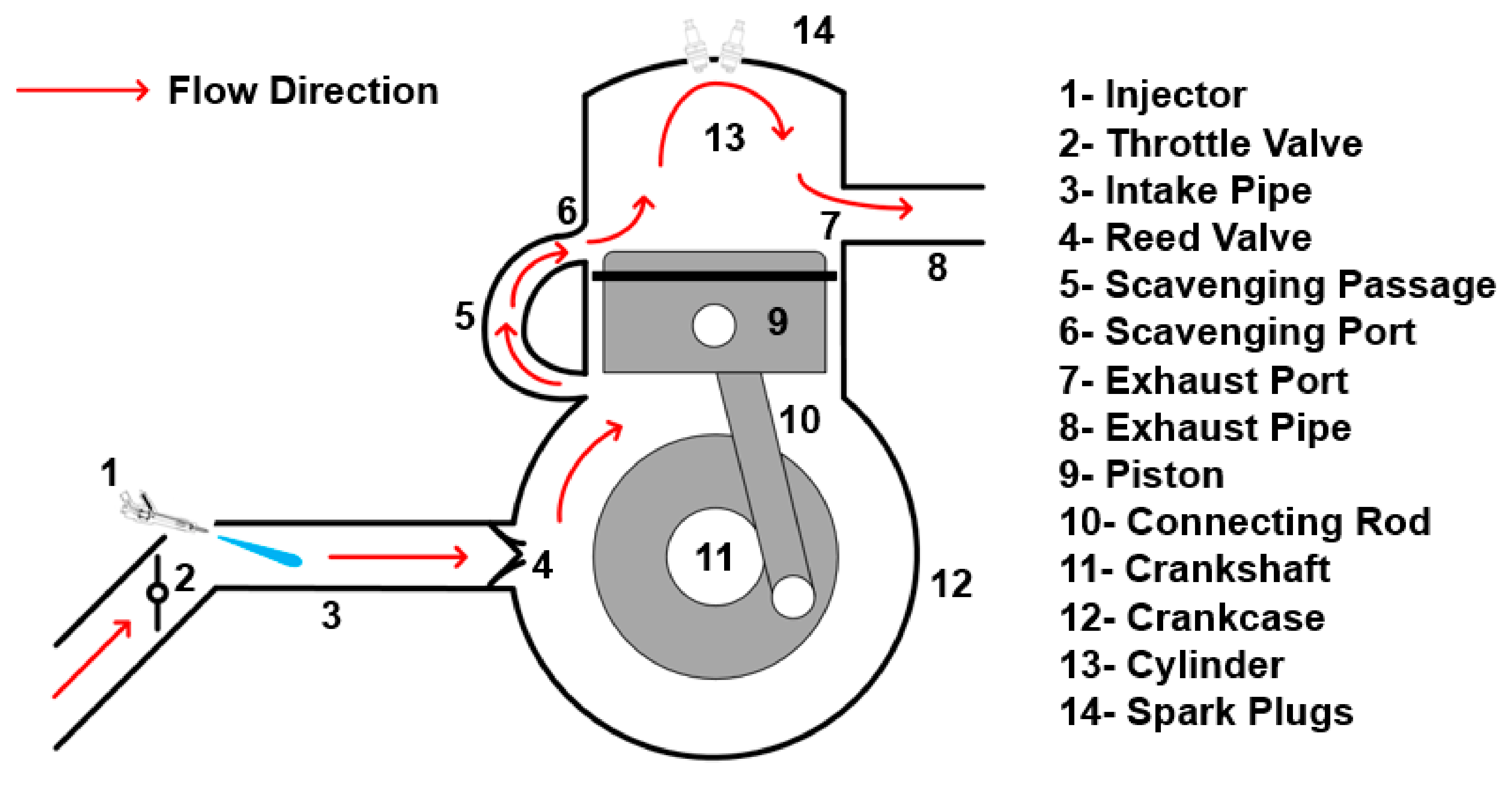
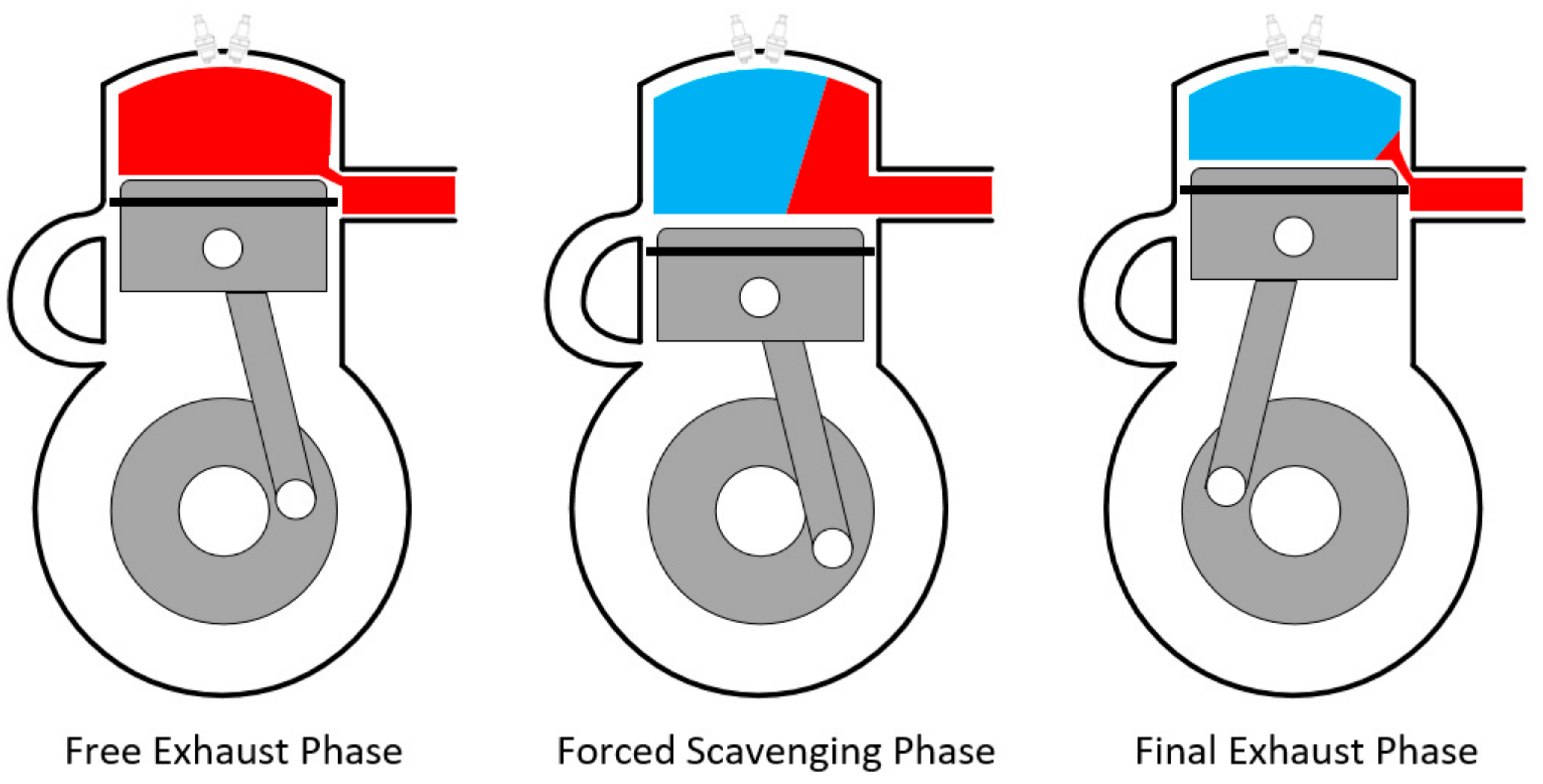
2.1. Working Principle of the Initial Prototype Engine
2.2. Working Principle of the Engine in the Relevant Reference (Reference Engine)
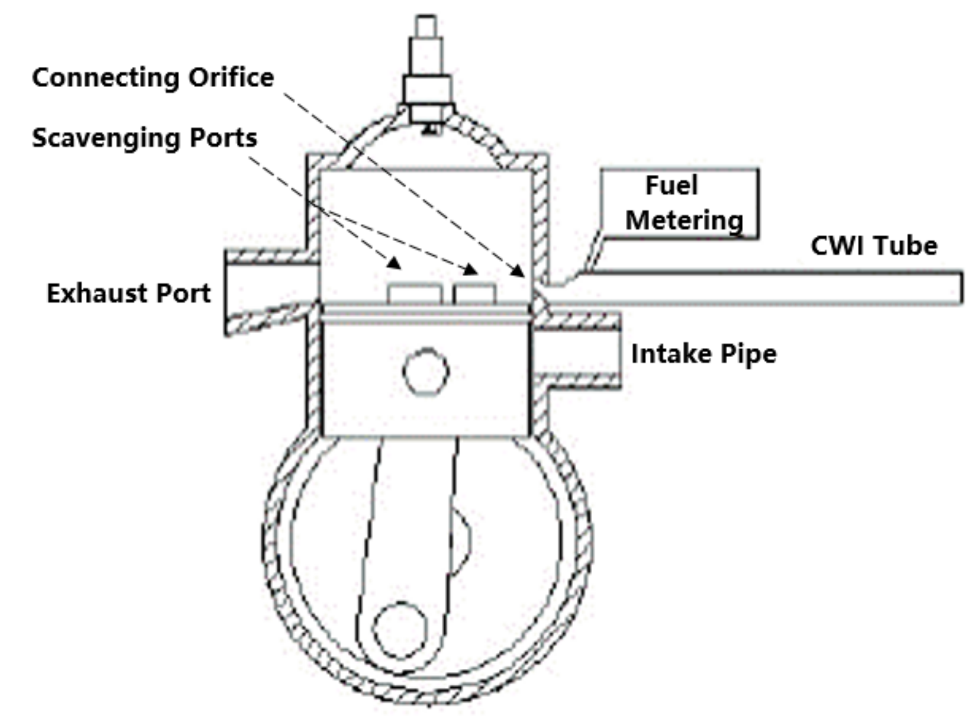
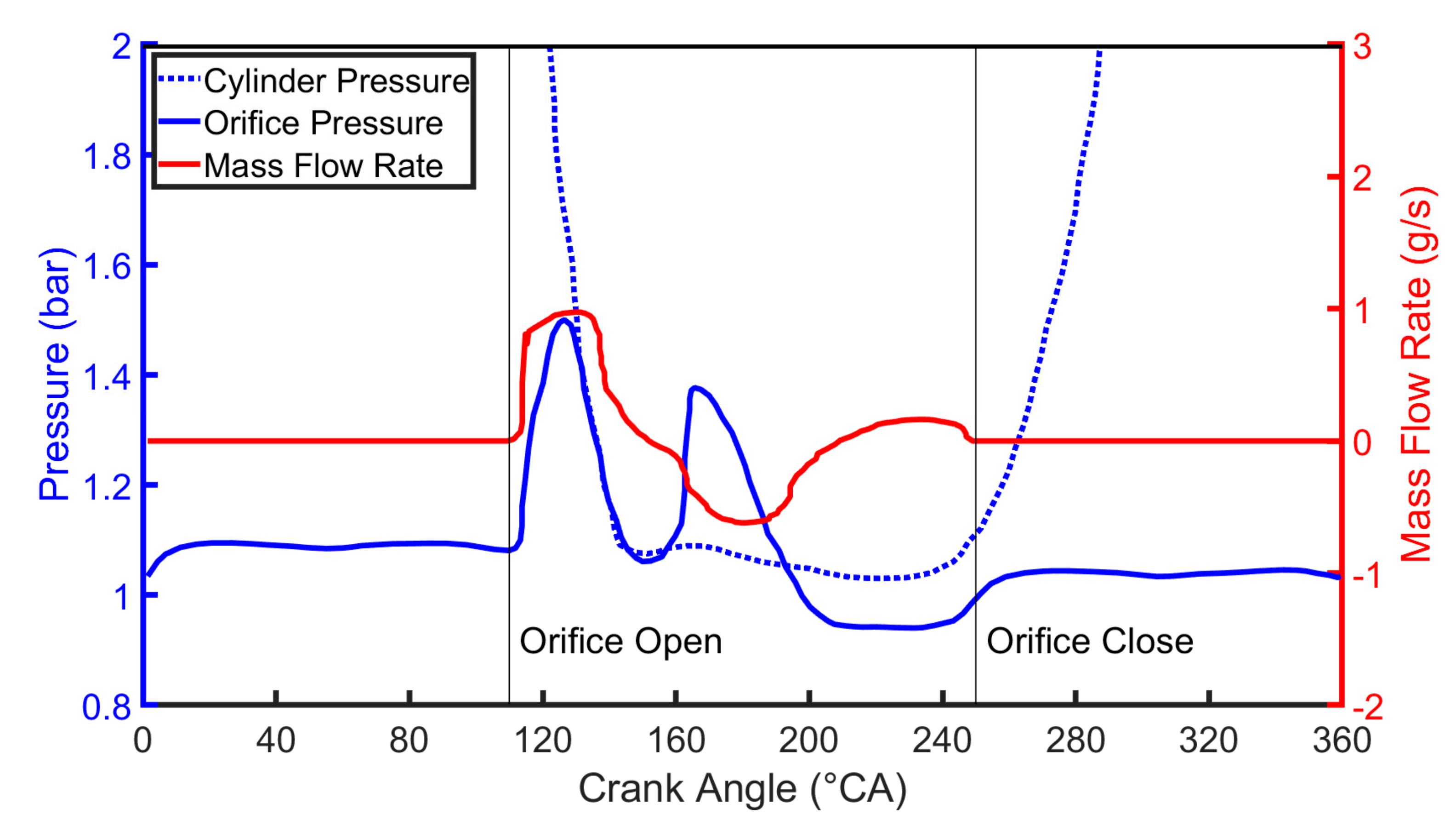
2.3. Working Principle of the Retrofitted Engine
3. Simulation and Experiment Platform Construction of the Initial Prototype Engine
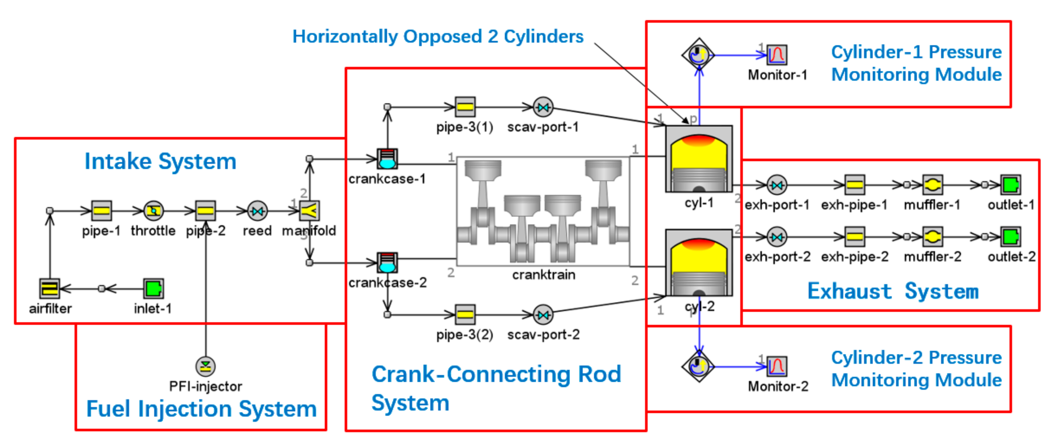
3.1. Simulation Platform Modeling of the Initial Prototype Engine
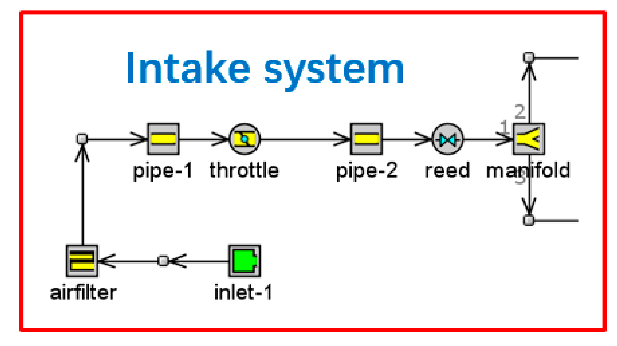
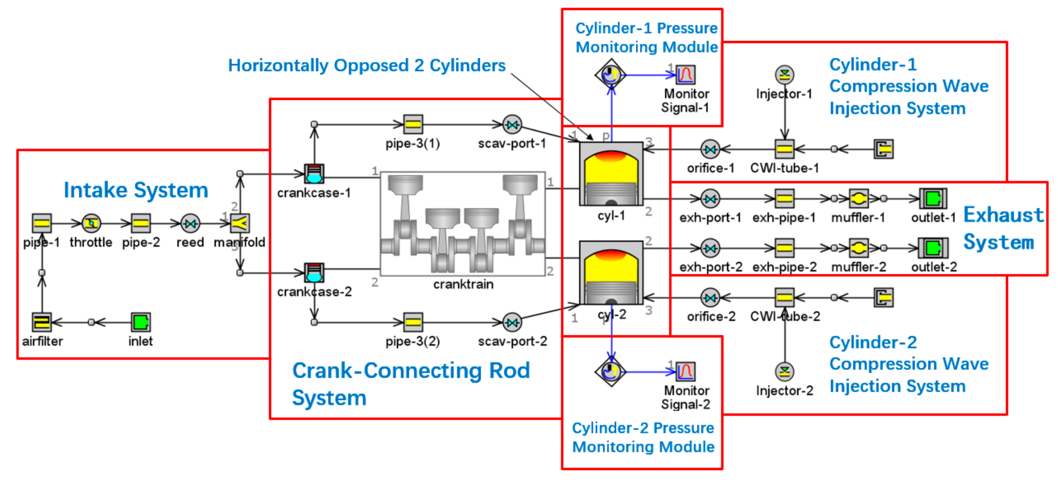
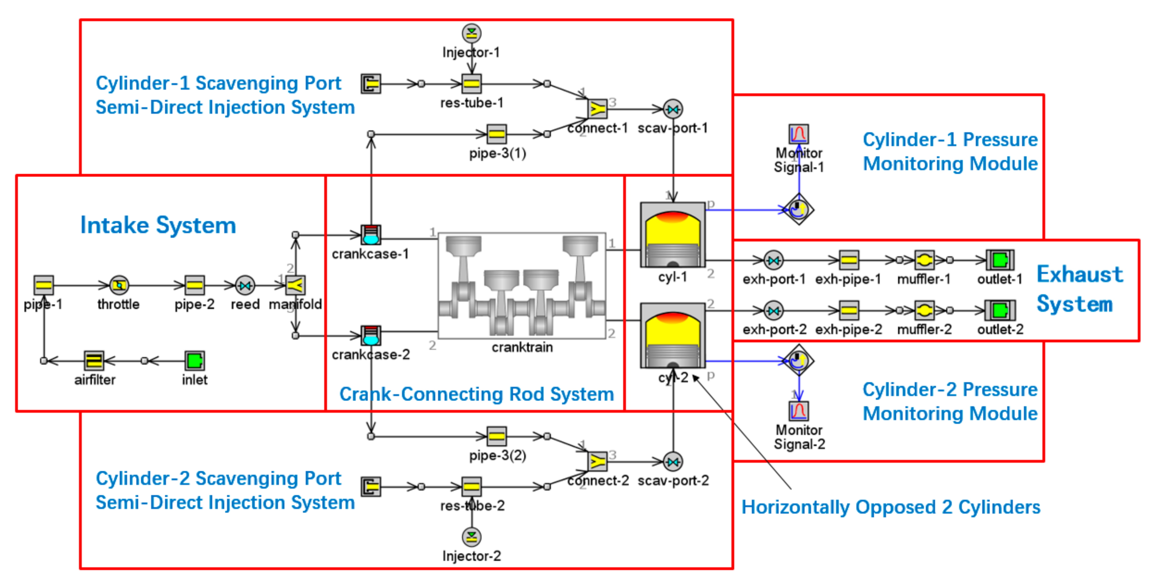
3.1.1. Intake System Modeling
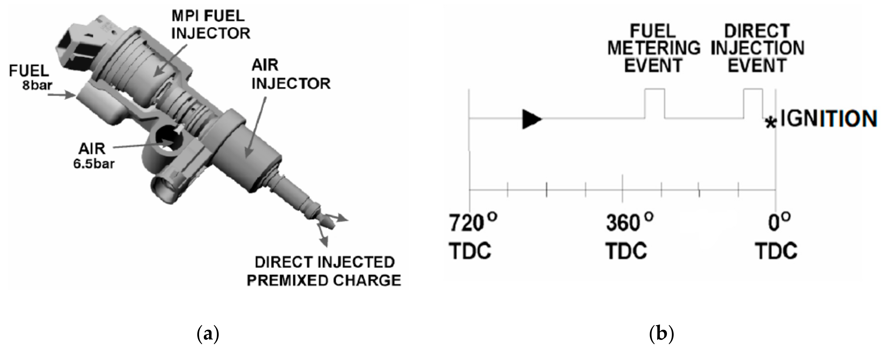
3.1.2. Fuel Injection System Modeling
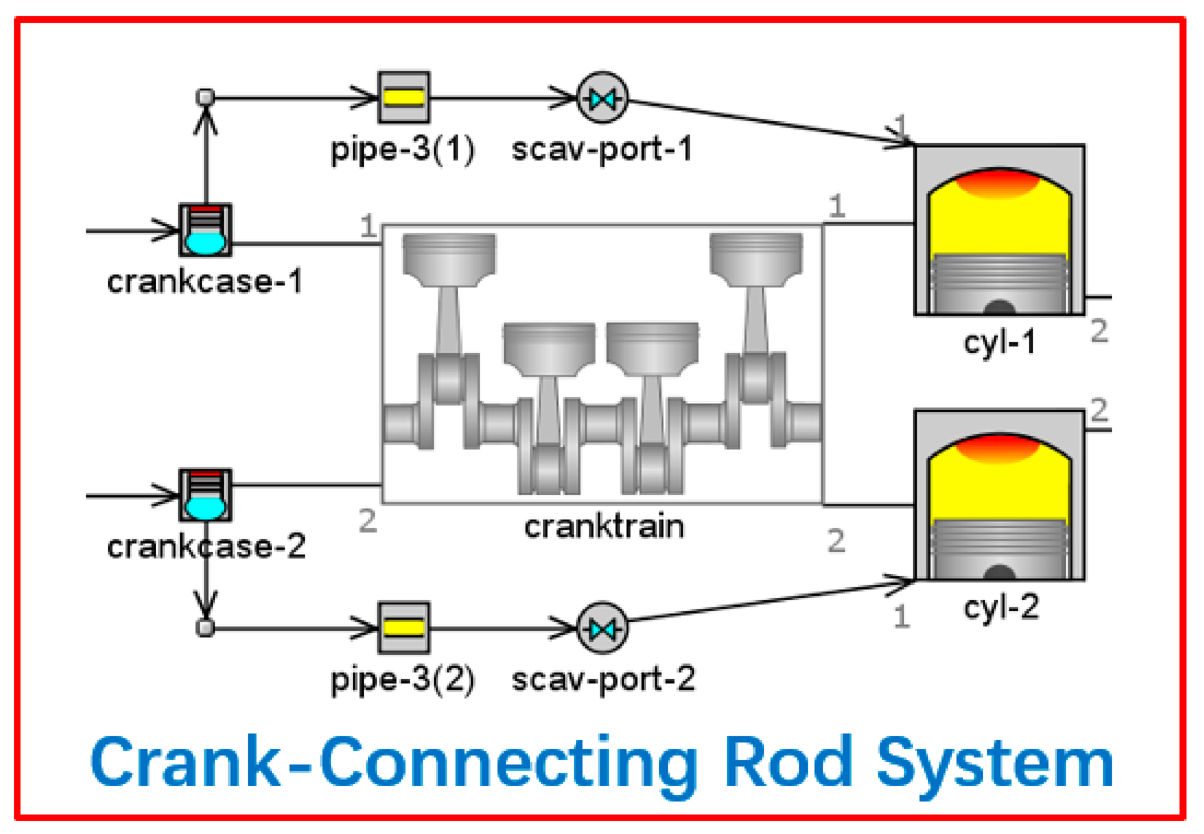
3.1.3. Crank-Connecting Rod System Modeling
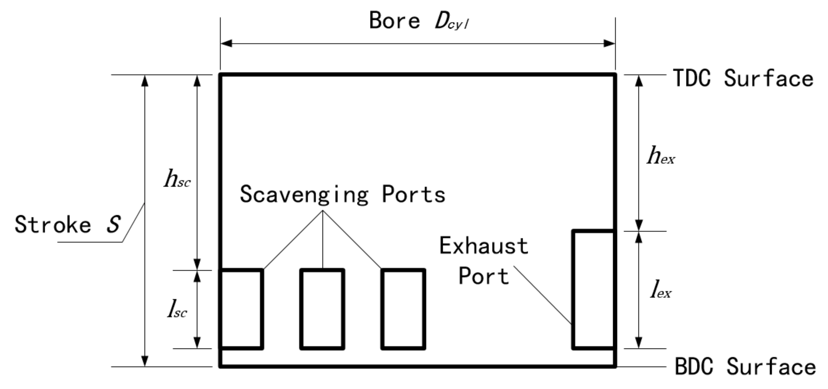
3.1.4. Cylinders Modeling
3.1.5. Exhaust System Modeling
3.1.6. Integrated Simulation Platform
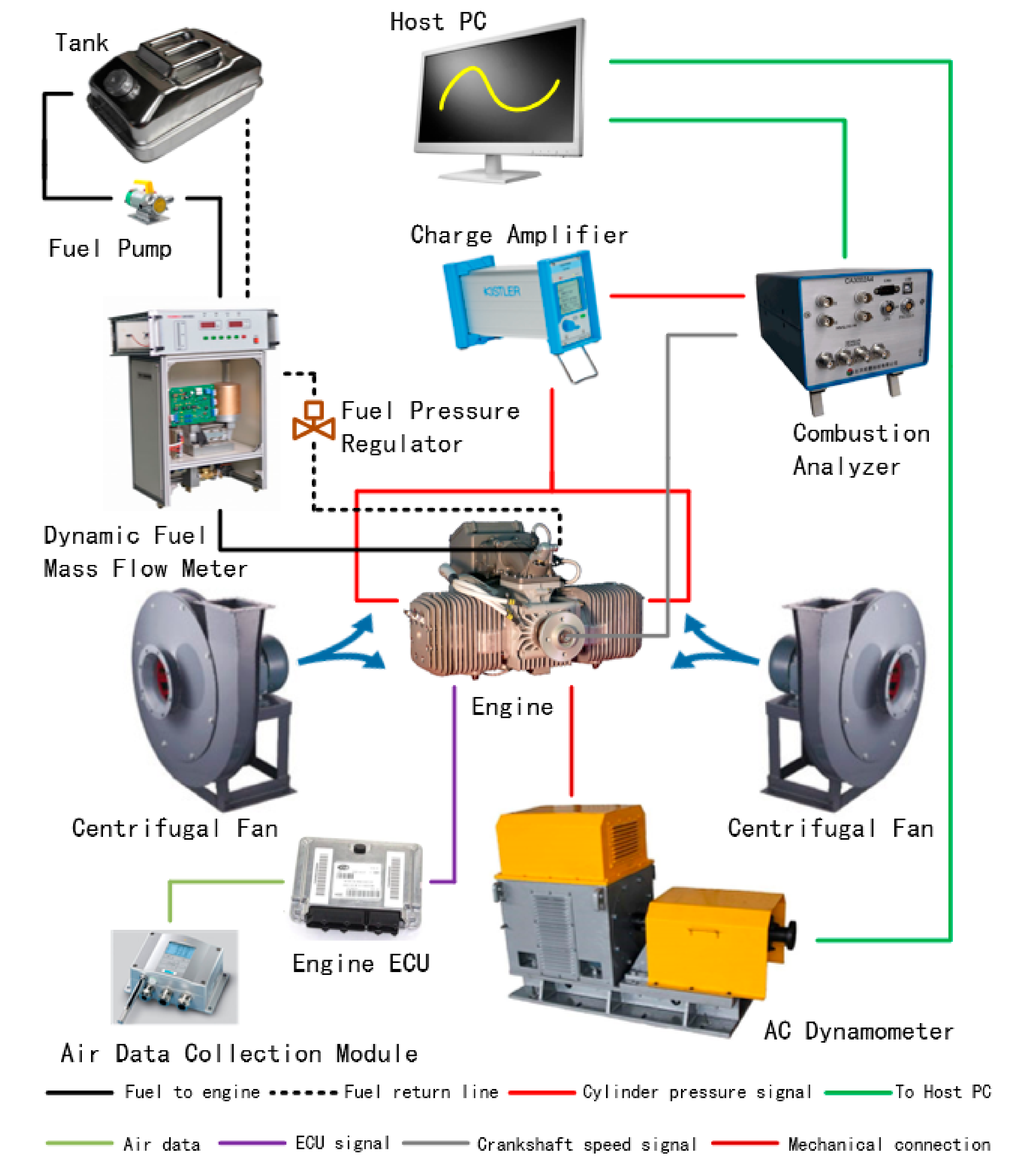
3.2. Experiment Platform Construction of the Initial Prototype Engine
4. Simulation Platform Calibration of the Initial Prototype Engine
4.1. Friction Loss Model Calibration
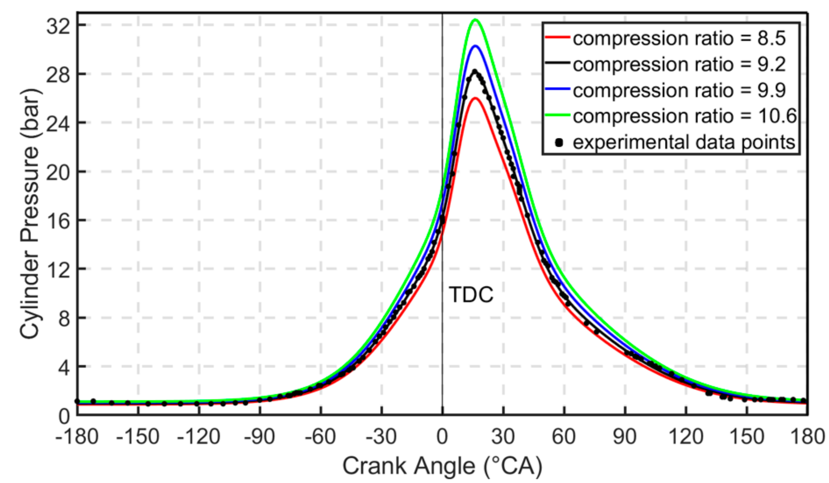
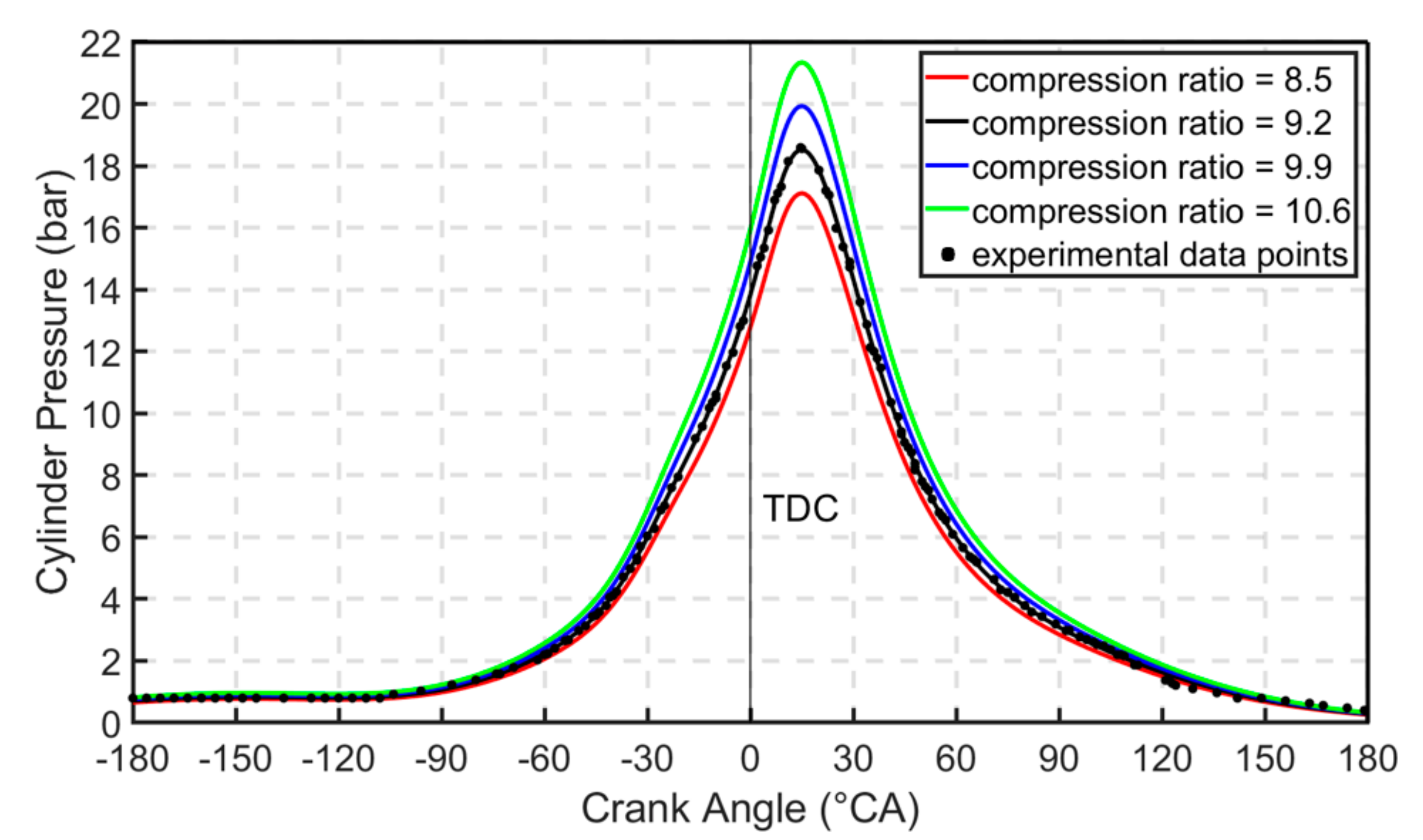
4.2. Effective Compression Ratio Calibration
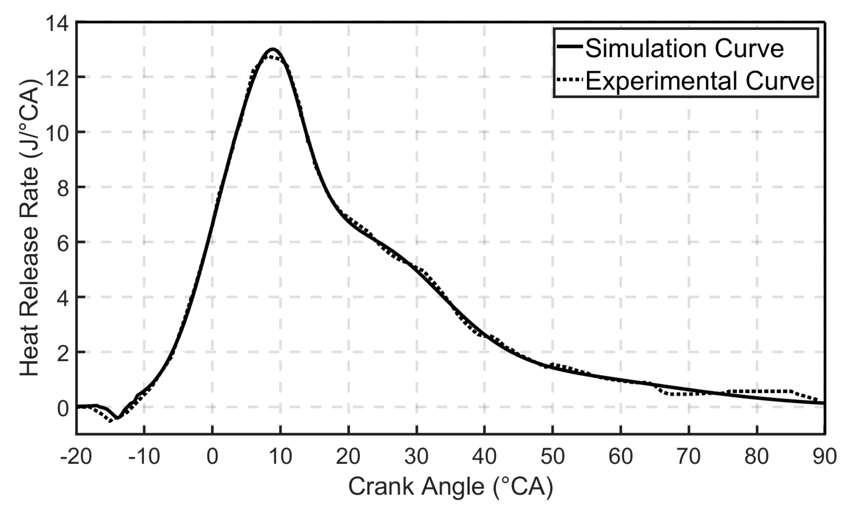
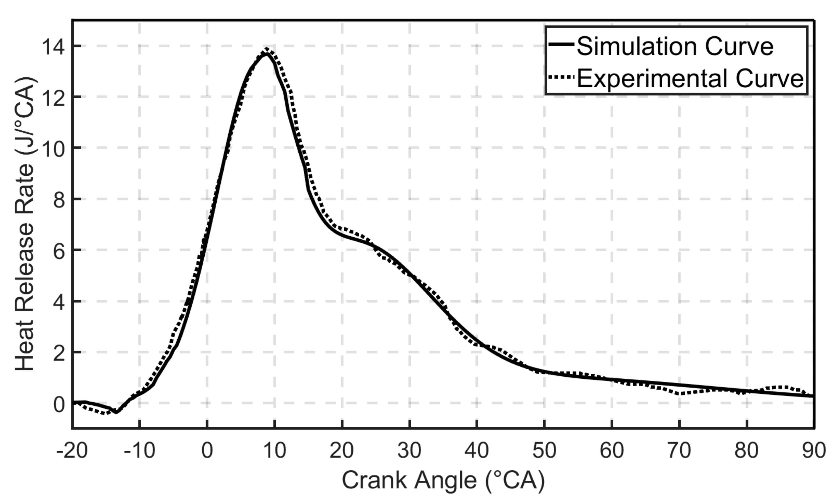
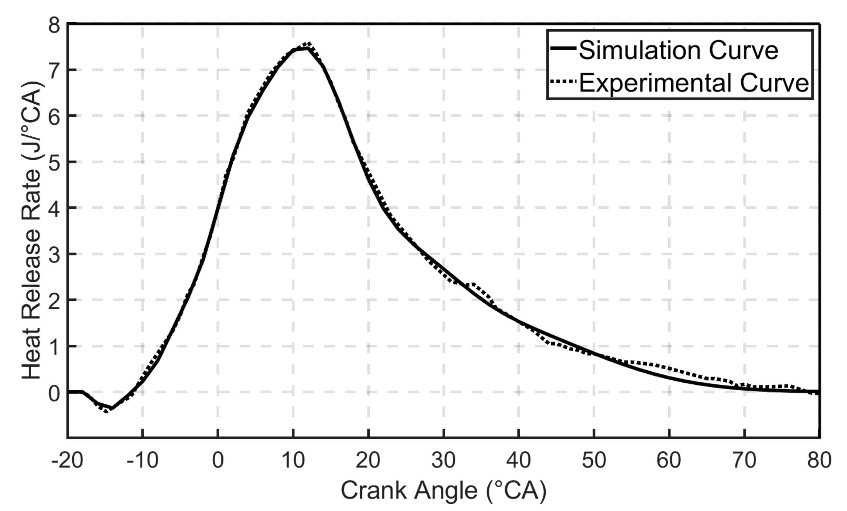
4.3. Heat Release Rate Curve Calibration
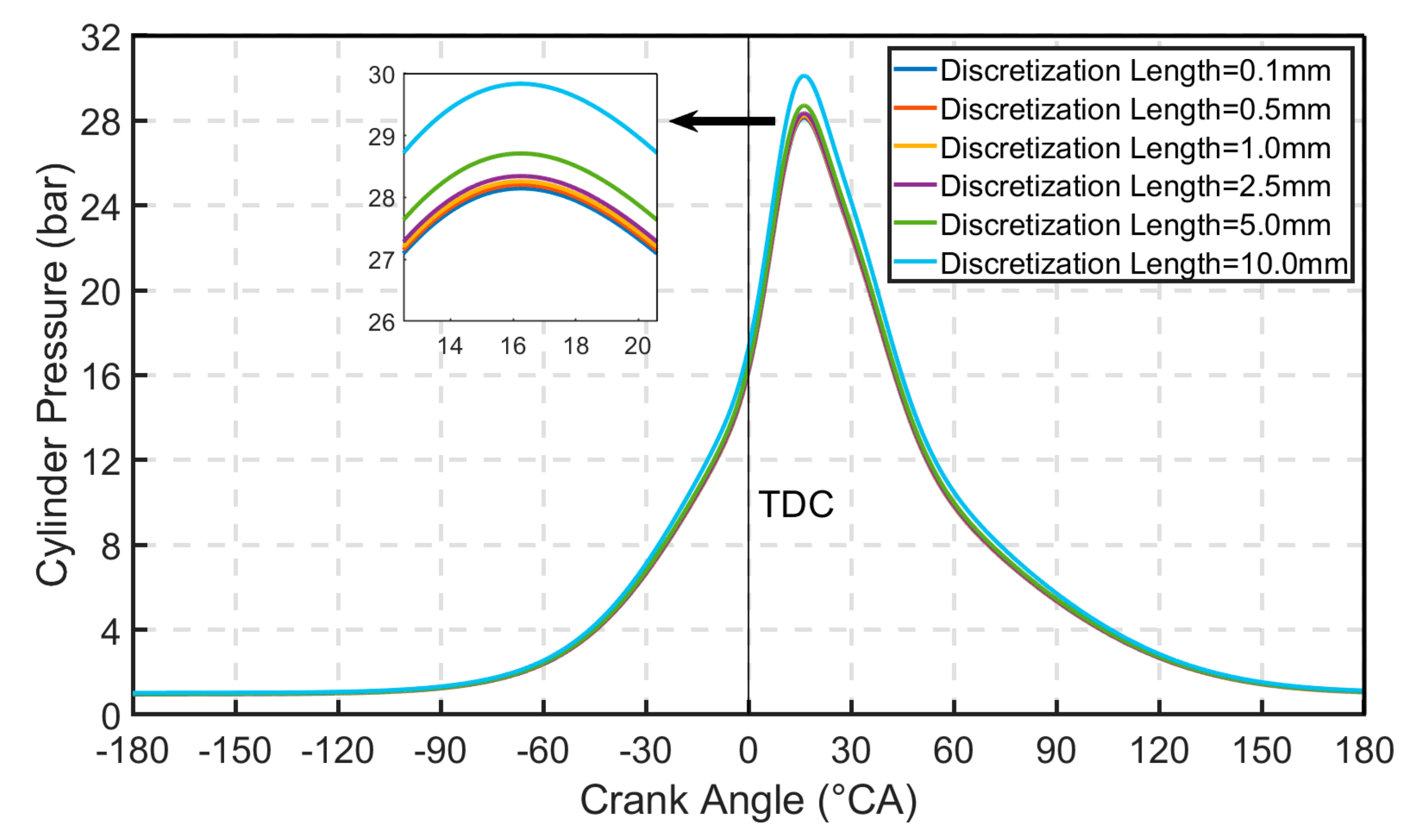
4.4. Discretization Length Calibration
5. Simulation Platform Construction of the Reference Engine and the Retrofitted Engine
5.1. Simulation Platform Construction of the Reference Engine
5.2. Simulation Platform Construction of the Retrofitted Engine
6. Simulation Results Analysis
6.1. Performance Comparison of the Initial Prototype Engine
6.2. Performance Comparison of the Three Types of Engines
7. Discussion
8. Conclusions
- (1)
- A preliminary comparison of the characteristics of all the three engines shows that the retrofitted engine has distinct advantages in many aspects such as the resonant intake system which offers considerable potential for increasing inlet flux, relatively high atomization quality of heavy fuel, and neither high mechanical processing difficulty nor a fuel pooling problem.
- (2)
- The modular modeling method provided by GT-SUITE can be adopted to establish the integrated simulation platforms of all the three engines. By dividing the engine into different subsystems, each part can be easily modeled using the dedicated simulation module. The graphical modeling simulation environment GT-ISE can not only shorten the modeling time, promote the modeling efficiency, but also improve system reliability, flexibility, transferability, and expandability.
- (3)
- To guarantee the accuracy of the established simulation platforms, the crucial parameter settings of corresponding models are calibrated against the obtained experimental data points, which also set the stage for subsequent comparative simulation.
- (4)
- Simulation results show that significant performance degradation (i.e., lower power, more fuel consumption) can be observed when the initial prototype engine is fueled with heavy fuel instead of regular gasoline. In addition, the retrofitted engine with the SPSDI system shows its superiority in performance evaluation indicators of both power and fuel economy over the other two types of engines (In terms of power performance, the brake power/brake torque/BMEP of the retrofitted engine are 3.3% higher than that of the initial prototype engine, while the reference engine offers an improvement of 2.1%. As for fuel economy performance, the BSFC of the retrofitted engine is 5.3% lower than that of the initial prototype engine, while the reference engine offers a reduction of 3.9%), which consequently verifies the feasibility of this proposed engine designing scheme.
Author Contributions
Funding
Acknowledgments
Conflicts of Interest
Abbreviation
| UAVs | unmanned aerial vehicles |
| 2SHFLA | 2-stroke heavy fuel light aeroengine |
| AADI | air assisted direct injection |
| MPI | multi-point port injection |
| TDC | top dead center |
| ISFC | indicated specific fuel consumption |
| BSFC | brake specific fuel consumption |
| 0-D | zero-dimensional |
| 3-D | three-dimensional |
| CFD | computational fluid dynamics |
| SMD | Sauter mean diameter |
| PFI | port fuel injection |
| CWI | compression wave injection |
| SPSDI | scavenging port semi-direct injection |
| GDI | gasoline direct injection |
| OEM | original equipment manufacturer |
| FMEP | friction mean effective pressure |
| IMEP | indicated mean effective pressure |
| BMEP | brake mean effective pressure |
| ECU | electronic control unit |
| FSR | full scale range |
| SV | simulation value |
| EV | experiment value |
| RG | regular gasoline |
| HF | heavy fuel |
Notation
| the mass flow rate of throttle valve | |
| throttle valve opening | |
| engine speed | |
| the pressure in pipe-2 | |
| flow coefficient | |
| the diameter of throttle valve | |
| the pressure in pipe-1 | |
| the temperature in pipe-1 | |
| the isentropic exponent of working substance | |
| , | intermediate variables in Equations (1) and (3) |
| , | intermediate variables in Equations (3) and (4) |
| , | constant coefficients in Equation (2) |
| constant coefficients in Equation (3) | |
| constant coefficients in Equation (4) | |
| Nusselt number | |
| Reynolds number | |
| instantaneous heat transfer coefficient | |
| bore | |
| mean piston speed | |
| cylinder pressure | |
| cylinder temperature | |
| flow velocity coefficient | |
| the coefficient of combustion chamber shape | |
| the temperature at the start of compression stroke | |
| the cylinder pressure at the start of compression stroke | |
| the cylinder volume at the start of compression stroke | |
| the displacement of a single cylinder | |
| the cylinder pressure under the motored condition | |
| the constant pressure term of FMEP in Equation (8) | |
| peak cylinder pressure factor | |
| mean piston speed factor | |
| mean piston speed squared factor | |
| maximum cylinder pressure | |
| stroke | |
| anchor angle | |
| combustion duration | |
| Wiebe exponent | |
| the burned fuel percentage at duration start | |
| the burned fuel percentage at anchor angle | |
| the burned fuel percentage at duration end | |
| burned start constant | |
| burned midpoint constant | |
| burned end constant | |
| Wiebe constant | |
| the start of combustion | |
| cumulative burn rate | |
| instantaneous crank angle | |
| the fraction of fuel burned | |
| geometric compression ratio | |
| the volume of combustion chamber on the cylinder head | |
| the length of scavenging ports | |
| the distance from TDC surface to scavenging ports | |
| the length of exhaust port | |
| the distance from TDC surface to exhaust port | |
| the end of combustion | |
| the total heat release from to | |
| heat release rate | |
| the heat transfer coefficient of combustion chamber wall | |
| the heat transfer area of combustion chamber wall | |
| the temperature of combustion chamber wall | |
| volumetric efficiency | |
| the reference density needed for calculating | |
| the imposed air–fuel ratio | |
| the delivery rate of injector |
Appendix A

References
- Finger, D.F.; Braurr, C.; Bil, C. Case studies in initial sizing for hybrid-electric general aviation aircraft. In Proceedings of the 2018 AIAA/IEEE Electric Aircraft Technologies Symposium (EATS), Cincinnati, OH, USA, 9–11 July 2018; pp. 1–22. [Google Scholar]
- Aldridge, E.C.; Stenbit, J.P. Unmanned Aerial Vehicles Roadmap 2002–2027; Department of Defense USA: Washington, DC, USA, 2002. [Google Scholar]
- Thiels, C.A.; Aho, J.M.; Zietlow, S.P.; Jenkins, D.H. Use of unmanned aerial vehicles for medical product transport. Air Med. J. 2015, 34, 104–108. [Google Scholar] [CrossRef] [PubMed]
- Zarándy, Á.; Zsedrovits, T.; Nagy, Z.; Kiss, A.; Roska, T. Visual sense-and-avoid system for UAVs. In Proceedings of the 2012 13th International Workshop on Cellular Nanoscale Networks and their Applications (CNNA), Turin, Italy, 29–31 August 2012; pp. 1–5. [Google Scholar]
- Cruzan, M.B.; Weinstein, B.G.; Grasty, M.R.; Kohrn, B.F.; Hendrickson, E.C.; Arredondo, T.M.; Thompson, P.G. Small unmanned aerial vehicles (micro-UAVs, drones) in plant ecology. Appl. Plant. Sci. 2016, 4, 1600041. [Google Scholar] [CrossRef] [PubMed]
- Crosbie, S.; Polanka, M.; Litke, P.; Hoke, J. Increasing reliability of a small 2-stroke internal combustion engine for dynamically changing altitudes. In Proceedings of the 50th AIAA Aerospace Sciences Meeting Including the New Horizons Forum and Aerospace Exposition, Nashville, TN, USA, 9–12 January 2012; p. 950. [Google Scholar]
- Sousa, J.; Paniagua, G.; Morata, E.C. Thermodynamic analysis of a gas turbine engine with a rotating detonation combustor. Appl. Energy 2017, 195, 247–256. [Google Scholar] [CrossRef]
- Bhangu, B.S.; Rajashekara, K. Control strategy for electric starter generators embedded in gas turbine engine for aerospace applications. In Proceedings of the IEEE Energy Conversion Congress and Exposition (ECCE), Phoenix, AZ, USA, 17–22 September 2011; pp. 1461–1467. [Google Scholar]
- Cirigliano, D. Engine-Type and Propulsion Configuration Selections for Long-Duration UAV Flights. Master’s Thesis, University of California, Irvine, CA, USA, 20 March 2017. [Google Scholar]
- Capata, R.; Marino, L.; Sciubba, E. A hybrid propulsion system for a high-endurance UAV: Configuration selection, aerodynamic study, and gas turbine bench tests. J. Unmanned Veh. Syst. 2014, 2, 16–35. [Google Scholar] [CrossRef]
- Husaboe, T.D.; Polanka, M.D.; Rittenhouse, J.A.; Litke, P.J.; Hoke, J.L. Dependence of Small Internal Combustion Engine’s Performance on Altitude. J. Propuls. Power 2014, 30, 1328–1333. [Google Scholar] [CrossRef]
- Hooper, P. Low Volatility Fuel Cold Start Experience with a Stepped Piston UAV Engine to Address Single Fuel Objectives; Technical Paper; SAE International: Detroit, MI, USA, 2017. [Google Scholar]
- Duddy, B.J.; Lee, J.; Walluk, M.; Hallbach, D. Conversion of a spark-ignited aircraft engine to JP-8 heavy fuel for use in unmanned aerial vehicles. SAE Int. J. Engines 2011, 4, 82–93. [Google Scholar] [CrossRef]
- Liu, R.; Wei, M.; Wang, C.; Huang, T. Fuel Flow Control for Starting a Crankcase-Injected Two-Stroke Spark Ignition Engine Fueled with Kerosene (RP-3). J. Energy Eng. 2019, 145, 04019010. [Google Scholar] [CrossRef]
- Feng, G.; Zhou, M. Assessment of heavy fuel aircraft piston engine types. J. Tsinghua Univ. 2016, 56, 1114–1121. [Google Scholar]
- Hooper, P. Experimental experience of cold starting a spark ignition UAV engine using low volatility fuel. Aircr. Eng. Aerosp. Technol. 2017, 89, 106–111. [Google Scholar] [CrossRef] [Green Version]
- Ma, S.; Li, N.; Hu, C. Present Status and Development Direction of Two Stroke Heavy Fuel Engine. Small Intern. Combust. Engine Veh. Tech. 2015, 44, 87–91. [Google Scholar]
- Gao, L.; Wang, H.; He, K. Application of Aviation Heavy Oil in Aviation Piston Engine. Small Intern. Combust. Engine Veh. Tech. 2018, 47, 84–89. [Google Scholar]
- Leighton, S.; Cebis, M.; Southern, M.; Ahern, S.; Horner, L. The OCP Small Engine Fuel Injection System for Future Two-Stroke Marine Engines; Technical Paper; SAE International: Detroit, MI, USA, 1994. [Google Scholar]
- Worth, D.; Coplin, N.; McNiff, M.; Stannard, M. Design Considerations for the Application of Air Assisted Direct In-Cylinder Injection Systems; Technical Paper; SAE International: Detroit, MI, USA, 1997. [Google Scholar]
- Houston, R.; Cathcart, G. Combustion and Emissions Characteristics of Orbital’s Combustion Process Applied to Multi-Cylinder Automotive Direct Injected 4-Stroke Engines; Technical Paper; SAE International: Detroit, MI, USA, 1998. [Google Scholar]
- Cathcart, G.; Zavier, C. Fundamental Characteristics of an Air-Assisted Direct Injection Combustion System as Applied to 4-Stroke Automotive Gasoline Engines; Technical Paper; SAE International: Detroit, MI, USA, 2000. [Google Scholar]
- Cathcart, G.; Dickson, G.; Ahern, S. The Application of Air-Assist Direct Injection for Spark-Ignited Heavy Fuel 2-Stroke and 4-Stroke Engines; Technical Paper; SAE International: Detroit, MI, USA, 2005. [Google Scholar]
- Groenewegen, J.R.; Sidhu, S.; Hoke, J.; Wilson, C.; Litke, P. The performance and emissions effects of utilizing heavy fuels and algae based biodiesel in a port-fuel-injected small spark ignition internal combustion engine. In Proceedings of the 47th AIAA/ASME/SAE/ASEE Joint Propulsion Conference & Exhibit, San Diego, CA, USA, 31 July–3 August 2012; p. 5807. [Google Scholar]
- Koci, C.; Florea, R.; Das, S.; Walls, M.; Simescu, S.; Roberts, C. Air-Assisted Direct Injection Diesel Investigations; Technical Paper; SAE International: Detroit, MI, USA, 2013. [Google Scholar]
- La, C.; Murphy, P.; Cakebread, S. Benchmarking a 2-Stroke Spark Ignition Heavy Fuel Engine; Technical Paper; SAE International: Detroit, MI, USA, 2012. [Google Scholar]
- Gao, H.; Zhang, F.; Wang, S. Experimental Study of Air-assisted Spray Characteristics of Aviation Kerosene Piston Engine. Acta Armamentarii 2019, 40, 927–937. [Google Scholar]
- Yang, H.; Chen, M.; Huang, L.; Hu, C. CFD simulation and experiment of transient spray for an air-assisted injector. J. Aerosp. Power 2015, 30, 2897–2903. [Google Scholar]
- Wang, S.; Yang, H. Simulation on Atomization Mechanism of Air-Assisted Injector for Aircraft Heavy Fuel Engine. Trans. CSICE 2018, 36, 127–135. [Google Scholar]
- Hu, C.; Wang, S.; Bi, Y.; Zhong, W. Combustion characteristics of direct injection piston aviation kerosene engine. J. Aerosp. Power 2017, 32, 1035–1042. [Google Scholar]
- Qiao, Y.; Duan, X.; Huang, K.; Song, Y.; Qian, J. Scavenging Ports’ Optimal Design of a Two-Stroke Small Aeroengine Based on the Benson/Bradham Model. Energies 2018, 11, 2739. [Google Scholar] [CrossRef] [Green Version]
- Ma, F.K.; Wang, J.; Feng, Y.N.; Zhang, Y.G.; Su, T.X.; Zhang, Y.; Liu, Y.H. Parameter Optimization on the Uniflow Scavenging System of an OP2S-GDI Engine Based on Indicated Mean Effective Pressure (IMEP). Energies 2017, 10, 368. [Google Scholar] [CrossRef] [Green Version]
- William, T.; Cobb, J. Compression Wave Injection: A Mixture Injection Method for Two-Stroke Engines Based on Unsteady Gas Dynamics; Technical Paper; SAE International: Detroit, MI, USA, 2001. [Google Scholar]
- Hoffmann, G.; Befrui, B.; Berndorfer, A.; Piock, W.F.; Varble, D.L. Fuel system pressure increase for enhanced performance of GDI multi-hole injection systems. SAE Int. J. Engines 2014, 7, 519–527. [Google Scholar] [CrossRef] [Green Version]
- Morel, T. Engine Performance Application Manual, GT-SUITE Version 2016; Gamma Technologies: Westmont, IL, USA, 2016. [Google Scholar]
- GT-SUITE—A Revolutionary MBSE Tool. Available online: http://www.gtisoft.com/ (accessed on 19 July 2020).
- Ouyang, M.; Li, J.; Yang, F.; Lu, L. Automotive New Powertrain: Systems, Models and Controls; Tsinghua University Press: Beijing, China, 2011. [Google Scholar]
- Hooper, P.R.; Al-Shemmeri, T. Improved efficiency of an unmanned air vehicle IC engine using computational modelling and experimental verification. Aircr. Eng. Aerosp. Technol. 2017, 89, 184–192. [Google Scholar] [CrossRef]
- Morel, T. Mechanics Theory Manual, GT-SUITE Version 2016; Gamma Technologies: Westmont, IL, USA, 2016. [Google Scholar]
- Shuai, S.; Wang, J. Automotive Engine Fundamentals; Tsinghua University Press: Beijing, China, 2014. [Google Scholar]
- Woschni, G. A Universally Applicable Equation for the Instantaneous Heat Transfer Coefficient in the Internal Combustion Engine; Technical Paper; SAE International: Detroit, MI, USA, 1967. [Google Scholar]
- Wiebe, I. Semi-Empirical Formula for the Combustion Rate in Fuel Processing and Combustion in Diesel Engines; Springer: Berlin, Germany, 1964. [Google Scholar]
- Chen, S.K.; Flynn, P.F. Development of a Single Cylinder Compression Ignition Research Engine; Technical Paper; SAE International: Detroit, MI, USA, 1965. [Google Scholar]
- Hooper, P.R.; Al-Shemmeri, T.; Goodwin, M.J. An experimental and analytical investigation of a multi-fuel stepped piston engine. J. Appl. Therm. Eng. 2012, 48, 32–40. [Google Scholar] [CrossRef]


| Parameters | Value |
|---|---|
| Engine Type | horizontally opposed 2-cylinder 2-stroke |
| Injection System | port fuel injection (PFI) |
| Ignition System | double programmed inductive discharging system |
| Intake system | naturally aspirated |
| Scavenging System | loop scavenging |
| Cooling System | forced air cooling |
| Lubrication System | mixed lubrication (2% synthetic oil) |
| Total Displacement | 0.500 L |
| Total Weight | 18.6 kg |
| Bore | 75 mm |
| Stroke | 56 mm |
| Compression Ratio | 10.6 |
| Rated Speed | 6500 r/min |
| Rated Torque | 42 N·m |
| Rated Power | 28.6 kW |
| Maximum Safety Speed | 6800 r/min |
| Minimum Steady Speed | 2200 r/min~2800 r/min |
| Operating Temperature | −20 °C–65 °C |
| Time Between Overhaul | 1000 h |
| Parameters | Value |
|---|---|
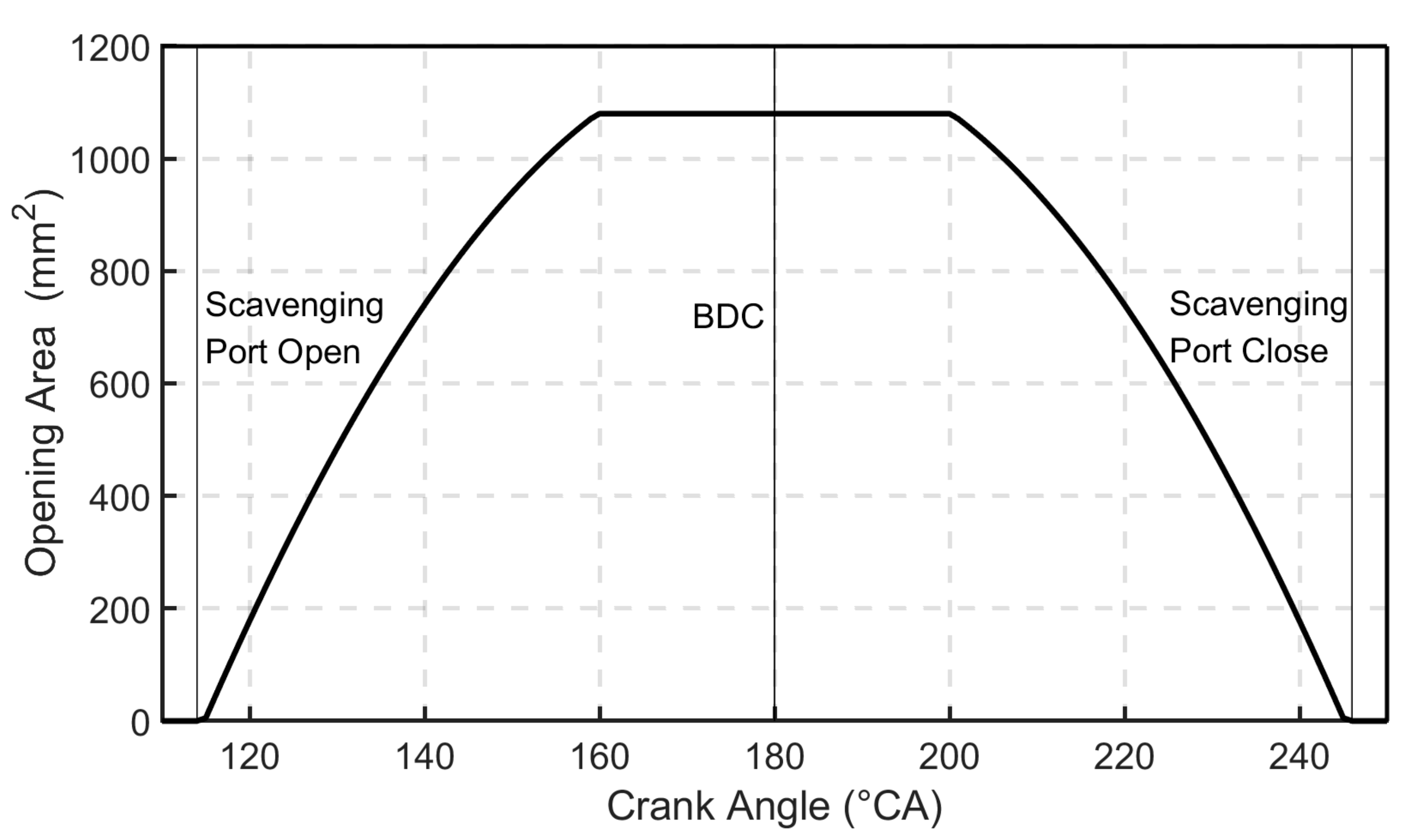
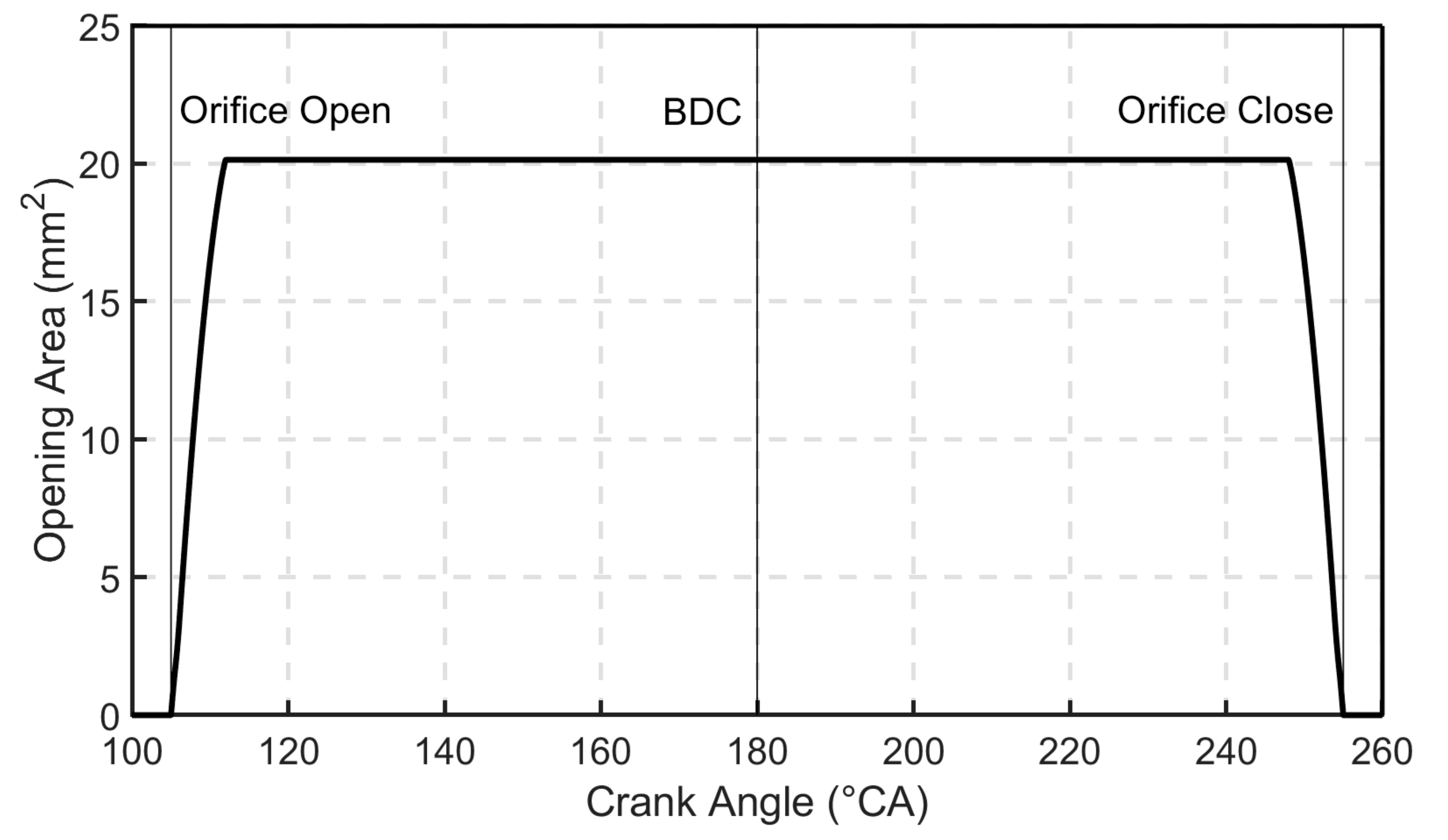
| Exhaust Port Open | 95 °CA |
| Scavenging Port Open | 114 °CA |
| Scavenging Port Close | 246 °CA |
| Exhaust Port Close | 265 °CA |
| Region | Value |
|---|---|
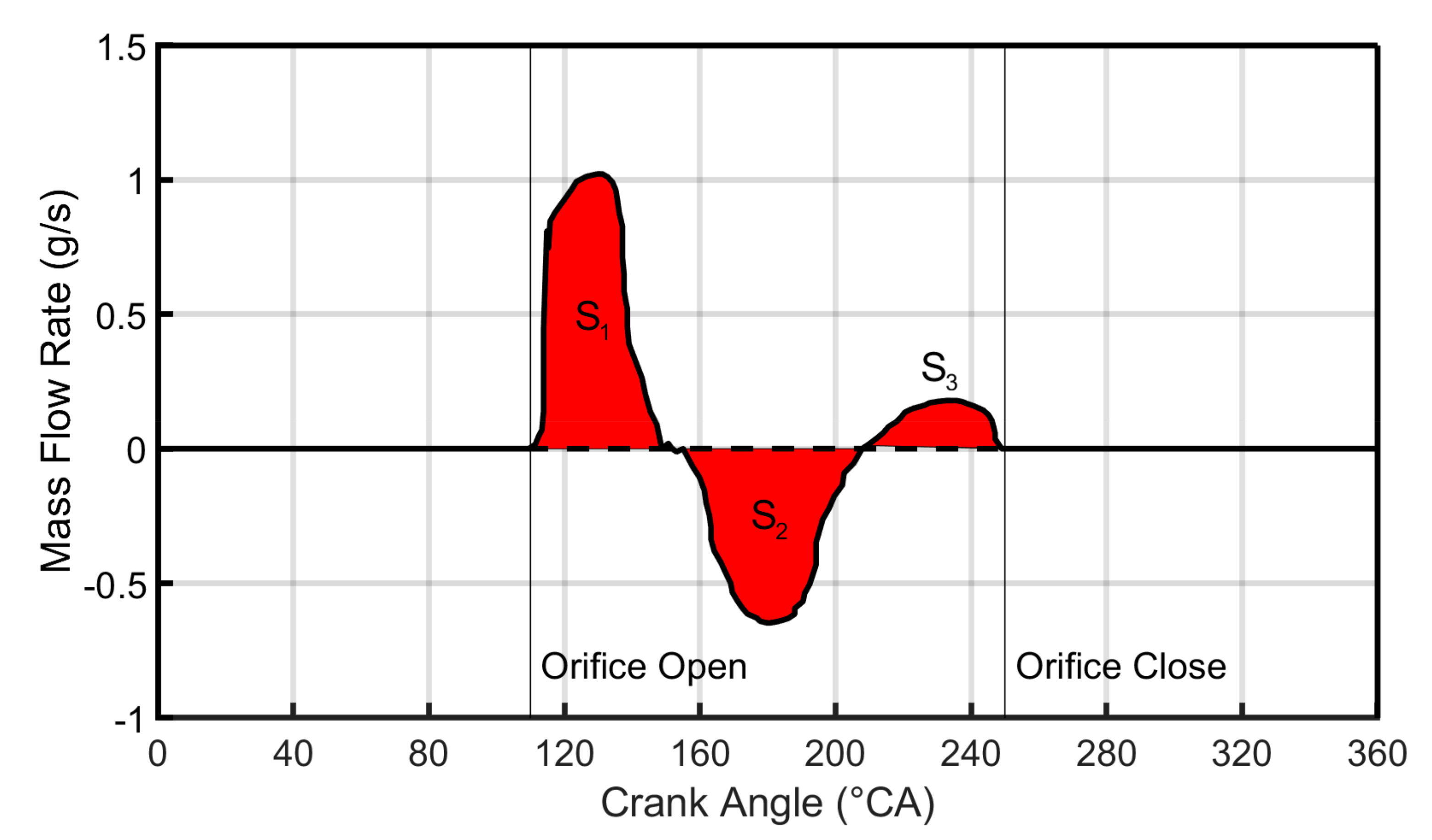
| S1 | 1.196 mg |
| S2 | 0.975 mg |
| S3 | 0.220 mg |
| Engine Type | Initial Prototype Engine | Reference Engine | Retrofitted Engine |
|---|---|---|---|
| Characteristics | |||
| Fuel Injection System Type | PFI | CWI | SPSDI |
| Forming Position of Air–Fuel Mixture | induct pipe | CWI tube | cylinder |
| Atomization Quality of Heavy Fuel | poor | good | good |
| Mechanical Processing Difficulty | No | high | low |
| Fuel Pooling Problem | No | Yes | No |
| Parameter | Value |
|---|---|
| Temperature | 300 K |
| Absolute Pressure | 1.013 bar |
| Composition | standard air |
| Parameter | Value | Parameter | Value |
|---|---|---|---|
| Valve Diameter | 45 mm | Diaphragm Mass | 0.54 g |
| Upstream Pressure Area | 1569.29 mm2 | Spring Stiffness | 1500 N/m |
| Downstream Pressure Area | 1437.38 mm2 | Pretension Setting Length | 10.7 mm |
| Initial Valve Lift | 0 mm | Seat Stiffness | 1.0 × 10⁸ N/m |
| Maximum Valve Lift | 8 mm | Stop Stiffness | 1.0 × 10⁸ N/m |
| Parameter | Value |
|---|---|
| Injector Location | 1.0 |
| Fuel Ratio Specification | air–fuel ratio |
| Injected Fluid Type | regular gasoline |
| Injected Fluid Temperature | 300 K |
| Vaporized Fluid Fraction | 30% |
| Parameter | Value |
|---|---|
| Crankcase Compression Ratio | 1.41 |
| Piston Skirt Temperature | 450 K |
| Cylinder Wall Temperature | 500 K |
| Crankcase Wall Temperature | 350 K |
| Heat Transfer Model | WoschniGT |
| Parameter | Value |
|---|---|
| Engine Type | 2-stroke |
| Speed or Load Specification | speed |
| Start of Cycle | 114 °CA Before TDC |
| Firing Interval | 0 °CA |
| Connecting Rod Length | 110 mm |
| Piston-to-Crank Offset | 0 mm |
| TDC Clearance Height | 0.4 mm |
| Friction Loss Model | EngFrctionCF |
| Parameter | Value |
|---|---|
| Stroke | 75 mm |
| Bore | 56 mm |
| Displacement of A Single Cylinder | 0.250 L |
| Head/Bore Area Ratio | 1.4 |
| Piston/bore Area Ratio | 1.1 |
| Cylinder Head Temperature | 550 K |
| Piston Surface Temperature | 550 K |
| Cylinder Wall Temperature | 500 K |
| Engine Combustion Model | EngCylCombSIWiebe |
| Engine Scavenging Model | EngCylScav |
| Experimental Equipment | Measurement Accuracy |
|---|---|
| Dynamic fuel mass flow meter | ±0.3% FSR |
| Charge amplifier | ±0.3% FSR |
| Combustion analyzer | ±0.5% FSR |
| AC dynamometer | ±0.2% FSR |
| Air data collection module | ±0.25% FSR |
| UAV Flight State | Operation Condition | Specification |
|---|---|---|
| Taking off | full load | throttle valve opening = 100% engine speed = 6500 r/min |
| Cruise | medium load | throttle valve opening = 60% engine speed = 5800 r/min |
| Landing | minimum load | throttle valve opening = 20% engine speed = 4500 r/min |
| Operation Condition | Brake Power (kW) | Brake Torque (N·m) | BMEP (bar) | Relative Error | |||
|---|---|---|---|---|---|---|---|
| SV | EV | SV | EV | SV | EV | ||
| minimum load | 11.10 | 10.92 | 23.55 | 23.16 | 2.96 | 2.91 | 1.68% |
| medium load | 24.55 | 24.21 | 40.43 | 39.87 | 5.13 | 5.06 | 1.38% |
| full load | 28.48 | 28.22 | 41.84 | 41.46 | 5.31 | 5.26 | 0.91% |
| Operation Condition | (bar) | (bar/(m/s)) | (bar/(m/s)2) | ||||
| minimum load | 0.27 | 0.0038 | 0.0021 | 0.0006 | |||
| medium load | 0.31 | 0.0042 | 0.0029 | 0.0010 | |||
| full load | 0.32 | 0.0045 | 0.0035 | 0.0012 | |||
| Operation Condition | Anchor Angle | Combustion Duration | Wiebe Exponent | Start of Combustion |
|---|---|---|---|---|
| Lull Load | 8.5 °CA After TDC | 32.5 °CA | 2.00 | 25.4 °CA Before TDC |
| Medium Load | 8.5 °CA After TDC | 32.0 °CA | 1.98 | 24.6 °CA Before TDC |
| Minimum Load | 10.5 °CA After TDC | 25.5 °CA | 1.92 | 15.4 °CA Before TDC |
| Discretization Length | Simulation Time (A Single Case) |
|---|---|
| 0.1 mm | 2254 s |
| 0.5 mm | 713 s |
| 1.0 mm | 259 s |
| 2.5 mm | 102 s |
| 5.0 mm | 84 s |
| 10.0 mm | 69 s |
| Property | 95 Octane Gasoline | RP-3 Aviation Kerosene |
|---|---|---|
| Molecular Weight | 113 | 141 |
| Flash point (°C) | −45–25 | 35–51 |
| Density (kg/L) | 0.70–0.75 | 0.73–0.82 |
| Kinematic viscosity at 20 °C (mm2/s) | 0.80 | 1.25 |
| Spontaneous ignition temperature (°C) | 510–530 | 275 |
| Stoichiometric air–fuel ratio | 14.70 | 14.65 |
| Low heat value (kg/kJ) | 44.07 | 43.35 |
| Engine Speed | Brake Power (kW) | Brake Torque (N·m) | IMEP (bar) | BMEP (bar) | ||||
|---|---|---|---|---|---|---|---|---|
| HF | RG | HF | RG | HF | RG | HF | RG | |
| 6500 r/min | 24.10 | 28.48 | 35.41 | 41.84 | 5.20 | 5.74 | 4.49 | 5.31 |
| 6000 r/min | 23.35 | 27.34 | 37.16 | 43.52 | 5.45 | 5.98 | 4.72 | 5.53 |
| 5500 r/min | 22.28 | 25.87 | 38.67 | 44.91 | 5.62 | 6.14 | 4.91 | 5.70 |
| 5000 r/min | 19.02 | 22.21 | 36.33 | 42.42 | 5.28 | 5.78 | 4.62 | 5.33 |
| 4500 r/min | 16.68 | 19.68 | 35.39 | 41.76 | 5.16 | 5.61 | 4.50 | 5.16 |
| 4000 r/min | 14.31 | 16.80 | 34.17 | 40.10 | 4.99 | 5.35 | 4.34 | 4.96 |
| 3500 r/min | 12.22 | 14.65 | 33.34 | 39.96 | 4.73 | 5.18 | 4.24 | 4.84 |
| 3000 r/min | 10.11 | 12.21 | 32.18 | 38.88 | 4.59 | 4.92 | 4.09 | 4.63 |
| Engine Speed | ISFC (g/kW·h) | BSFC (g/kW·h) | Peak Pressure (bar) | Crank Angle at the Peak Pressure (°CA) | ||||
|---|---|---|---|---|---|---|---|---|
| HF | RG | HF | RG | HF | RG | HF | RG | |
| 6500 r/min | 387.27 | 350.84 | 448.51 | 379.25 | 28.65 | 28.85 | 14.84 | 14.78 |
| 6000 r/min | 383.86 | 349.84 | 443.23 | 378.31 | 29.54 | 29.97 | 14.91 | 14.93 |
| 5500 r/min | 391.15 | 358.02 | 447.71 | 385.66 | 30.24 | 30.68 | 14.99 | 15.05 |
| 5000 r/min | 393.21 | 359.19 | 449.38 | 389.52 | 30.45 | 30.90 | 14.93 | 14.96 |
| 4500 r/min | 388.63 | 357.46 | 445.63 | 388.63 | 31.27 | 31.70 | 15.04 | 15.08 |
| 4000 r/min | 392.01 | 365.63 | 450.72 | 394.38 | 31.59 | 32.08 | 14.92 | 14.99 |
| 3500 r/min | 406.22 | 370.93 | 453.17 | 396.99 | 30.53 | 30.97 | 14.91 | 14.89 |
| 3000 r/min | 409.86 | 382.37 | 459.97 | 406.32 | 32.58 | 33.05 | 15.12 | 15.10 |
| Engine Load (Throttle Valve Opening) | Brake Power (kW) | Brake Torque (N·m) | IMEP (bar) | BMEP (bar) | ||||
|---|---|---|---|---|---|---|---|---|
| HF | RG | HF | RG | HF | RG | HF | RG | |
| 100% | 24.10 | 28.48 | 35.41 | 41.84 | 5.20 | 5.74 | 4.49 | 5.31 |
| 60% | 22.59 | 26.86 | 33.19 | 39.46 | 4.95 | 5.45 | 4.34 | 5.01 |
| 45% | 20.57 | 24.71 | 30.22 | 36.31 | 4.55 | 5.12 | 3.95 | 4.61 |
| 35% | 17.60 | 21.58 | 25.85 | 31.7 | 3.98 | 4.57 | 3.38 | 4.03 |
| 30% | 15.68 | 19.55 | 23.04 | 28.72 | 3.60 | 4.11 | 3.01 | 3.65 |
| 25% | 13.09 | 16.81 | 19.23 | 24.69 | 3.10 | 3.58 | 2.51 | 3.14 |
| 20% | 10.73 | 14.32 | 15.77 | 21.04 | 2.64 | 3.09 | 2.06 | 2.67 |
| 10% | 6.35 | 9.70 | 9.33 | 14.25 | 1.79 | 2.20 | 1.22 | 1.81 |
| Engine Load (Throttle Valve Opening) | ISFC (g/kW·h) | BSFC (g/kW·h) | Peak Pressure (bar) | Crank Angle at the Peak Pressure (°CA) | ||||
|---|---|---|---|---|---|---|---|---|
| HF | RG | HF | RG | HF | RG | HF | RG | |
| 100% | 387.27 | 350.84 | 448.51 | 379.25 | 28.65 | 28.85 | 14.84 | 14.78 |
| 60% | 376.37 | 341.84 | 429.27 | 371.86 | 27.52 | 27.72 | 14.72 | 14.69 |
| 45% | 383.45 | 340.76 | 441.69 | 378.46 | 26.12 | 26.29 | 14.45 | 14.46 |
| 35% | 386.19 | 336.34 | 454.75 | 381.40 | 24.17 | 24.30 | 14.01 | 14.13 |
| 30% | 393.75 | 344.89 | 470.93 | 388.36 | 22.93 | 23.05 | 13.70 | 13.79 |
| 25% | 397.75 | 344.42 | 491.25 | 392.69 | 21.24 | 21.33 | 13.22 | 13.28 |
| 20% | 405.27 | 346.25 | 519.38 | 400.72 | 19.65 | 19.72 | 12.57 | 12.63 |
| 10% | 379.23 | 308.55 | 556.41 | 375.04 | 16.78 | 16.82 | 10.87 | 11.03 |
| Performance Indicators | Initial Prototype Engine | Reference Engine | Retrofitted Engine |
|---|---|---|---|
| Brake Power (kW) | 7.85 | 8.02 | 8.11 |
| Brake Torque (N·m) | 16.66 | 17.02 | 17.21 |
| IMEP/BMEP (bar) | 2.59/2.11 | 2.62/2.16 | 2.63/2.18 |
| ISFC/BSFC (g/kW·h) | 425.59/522.38 | 413.82/501.95 | 410.03/494.67 |
| Peak Pressure (bar) | 18.59 | 20.37 | 20.61 |
| Crank Angle at the Peak Pressure (°CA) | 14.64 | 10.55 | 10.08 |
| Performance Indicators | Initial Prototype Engine | Reference Engine | Retrofitted Engine |
|---|---|---|---|
| Brake Power (kW) | 20.88 | 21.25 | 21.33 |
| Brake Torque (N·m) | 34.38 | 34.99 | 35.12 |
| IMEP/BMEP (bar) | 4.89/4.36 | 4.95/4.44 | 4.97/4.46 |
| ISFC/BSFC (g/kW·h) | 372.11/417.34 | 367.42/409.62 | 359.64/400.77 |
| Peak Pressure (bar) | 26.41 | 29.29 | 29.56 |
| Crank Angle at the Peak Pressure (°CA) | 14.94 | 10.98 | 10.27 |
| Performance Indicators | Initial Prototype Engine | Reference Engine | Retrofitted Engine |
|---|---|---|---|
| Brake Power (kW) | 24.10 | 24.42 | 24.66 |
| Brake Torque (N·m) | 35.41 | 35.88 | 36.23 |
| IMEP/BMEP (bar) | 5.20/4.49 | 5.24/4.55 | 5.27/4.60 |
| ISFC/BSFC (g/kW·h) | 387.27/448.51 | 381.19/439.13 | 373.33/428.35 |
| Peak Pressure (bar) | 28.65 | 32.06 | 32.75 |
| Crank Angle at the Peak Pressure (°CA) | 14.84 | 10.96 | 10.21 |
© 2020 by the authors. Licensee MDPI, Basel, Switzerland. This article is an open access article distributed under the terms and conditions of the Creative Commons Attribution (CC BY) license (http://creativecommons.org/licenses/by/4.0/).
Share and Cite
Qiao, Y.; Lin, L.; Zhong, W.; Huang, K. Investigation on the Performance Characteristics of 2-Stroke Heavy Fuel Light Aeroengine (2SHFLA) with Different Fuel Injection Systems: Modeling and Comparative Simulation. Energies 2020, 13, 5136. https://doi.org/10.3390/en13195136
Qiao Y, Lin L, Zhong W, Huang K. Investigation on the Performance Characteristics of 2-Stroke Heavy Fuel Light Aeroengine (2SHFLA) with Different Fuel Injection Systems: Modeling and Comparative Simulation. Energies. 2020; 13(19):5136. https://doi.org/10.3390/en13195136
Chicago/Turabian StyleQiao, Yuan, Li Lin, Wei Zhong, and Kaisheng Huang. 2020. "Investigation on the Performance Characteristics of 2-Stroke Heavy Fuel Light Aeroengine (2SHFLA) with Different Fuel Injection Systems: Modeling and Comparative Simulation" Energies 13, no. 19: 5136. https://doi.org/10.3390/en13195136
APA StyleQiao, Y., Lin, L., Zhong, W., & Huang, K. (2020). Investigation on the Performance Characteristics of 2-Stroke Heavy Fuel Light Aeroengine (2SHFLA) with Different Fuel Injection Systems: Modeling and Comparative Simulation. Energies, 13(19), 5136. https://doi.org/10.3390/en13195136