Simulations of Aerodynamic Separated Flows Using the Lattice Boltzmann Solver XFlow

Abstract

We present simulations of turbulent detached flows using the commercial lattice Boltzmann solver XFlow (by Dassault Systemes). XFlow’s lattice Boltzmann formulation together with an efficient octree mesh generator reduce substantially the cost of generating complex meshes for industrial flows. In this work, we challenge these meshes and quantify the accuracy of the solver for detached turbulent flows. The good performance of XFlow when combined with a Large-Eddy Simulation turbulence model is demonstrated for different industrial benchmarks and validated using experimental data or fine numerical simulations. We select five test cases: the Backward-facing step the Goldschmied Body the HLPW-2 (2nd High-Lift Prediction Workshop) full aircraft geometry, a NACA0012 under dynamic stall conditions and a parametric study of leading edge tubercles to improve stall behavior on a 3D wing.

1. Introduction

Aerodynamic performance plays a major role in the design process of an aircraft. The aeronautical industry has been using Computation Fluid Dynamics (CFD) as a complement to wind tunnel measurements, which are typically executed at the end of the production cycle. CFD studies present a strong advantage, as they allow several design iterations before manufacturing the product and therefore help to decrease manufacturing costs drastically. The analysis of an aircraft relies on its aerodynamic performance in linear regime, i.e., at low angles of attack. However, aircraft also require to maintain aerodynamic performance at high angles of attack, to ensure safety and stability at taking-off, landing or under extreme weather conditions.

Presently, Navier-Stokes (N-S) solvers (using Reynolds Averaged Navier-Stokes (RANS) turbulence models) are able to predict, with high accuracy, linear aerodynamic performance at low angles of attack. However these solvers face strong difficulties and limitations when predicting aerodynamics near stall, which can be explained by the following reasons. First, the wing geometry of an aircraft in high-lift configuration is complex since the flap and slat are deflected, and thus it is extremely difficult to mesh in the gap between the wing and the flap or slat. Second, the flow is highly unsteady and separated, and standard turbulence models (such as RANS) fail to predict accurately flow separation. These two reasons make the solution convergence difficult or even impossible in most cases. Please note that the dependence of the flow accuracy and the quality of the mesh in N-S solvers as been widely explored in the past, e.g., [1,2].

Traditional CFD, using RANS closure models, were employed for decades in industry where robust and efficient simulation processes were established. Along these lines, several numerical treatments were proposed to enhance robustness of the N-S equations in complex engineering problems. For example, pressure-velocity decoupling in incompressible flows [3], multiphase multi-component flows [4] or shock-turbulence interaction [5] helped to obtain flow solutions and aerodynamic coefficients in complex flows. However, these traditional solvers face limitations especially related to the mesh, to model moving geometries with complex motions, or when strongly unsteady and separated flows are involved. The lattice Boltzmann Method (LBM) presents an alternative to classic finite volumes methods and shows promise to address some of these limitations, such as detached unsteady flows. Several works presented promising LBM flows over complex geometries with separated flows [6,7,8,9]. More challenging simulations including moving geometries were addressed in [10,11], and fluid-structure interactions in [12].

To illustrate the ability of the LBM to solve industrial problems with detached flows, XFlow is used to simulate five cases: the Backward-facing step [13], the Goldschmied Body [14], the HLPW-2 (2nd High-Lift Prediction Workshop) [15], dynamic stall for a NACA0012 [16] and a 3D wing with leading-edge tubercles [17].

The content of this text is organized as follows. First, Section 2 introduces the LBM with the different models implemented in XFlow. Then, Section 3 describes various test cases with XFlow setup and numerical results. Finally, Section 4 summarizes the main conclusions of the work.

2. Numerical Methodology

2.1. Lattice Boltzmann Method

The lattice Boltzmann method solves Boltzmann’s transport equation using probability distribution functions, f, to describe the mesoscopic scale of fluid flow [18]. The method uses a collision-streaming scheme to solve the discrete Boltzmann equation:

$$f_i(\mathbf{x}+{\mathbf{e}}_{\mathbf{i}}\Delta t,t+\Delta t)-f_i(\mathbf{x},t)=\Delta t{\mathsf{\Omega }}_i(\mathbf{x},t),i=0,\dots ,Q-1,$$

(1)

where $f_i$ is the probability distribution functions in the direction i, Q is the number of velocity directions, $\mathbf{x}$ is the position vector, ${\mathbf{e}}_{\mathbf{i}}=(e_{ix},e_{iy},e_{iz})$ is the discrete velocity direction vector and ${\mathsf{\Omega }}_i$ is the collision operator. The first two terms are called streaming steps while the right hand side includes the collision operator.

The stream-and-collide approach is posed over lattices, which are constructed of Cartesian points with a discrete set of velocity directions. The lattice scheme is usually denoted as DnQm where n represents the dimension of the problem, and m the number of velocity directions. However, XFlow is a LBM solver based on the D3Q27 lattice scheme with a central moment collision operator [19], which enhances the numerical stability compared with standard LBM [20,21].

The macroscopic variables are calculated using the statistical moments, ${\mu }_{x^k{y}^l{z}^m}$, defined by the following relation:

$${\mu }_{x^k{y}^l{z}^m}=\sum _{i=1}^Q{f}_i{e}_{ix}^k{e}_{iy}^l{e}_{iz}^m,$$

(2)

where k, l, and m are the orders of the moments in the x, y, and z directions, respectively, which leads to the moment order: $k+l+m$. For example, the moment of order zero provides the density, and the moment of order one provides the momentum:

$$\begin{array}{c}\hfill {\mu }_{x^0{y}^0{z}^0}=\sum _{i=1}^Q{f}_i=\rho ,{\mu }_{x^1{y}^0{z}^0}=\sum _{i=1}^Q{f}_i{\mathbf{e}}_{ix}=\rho u_x.\end{array}$$

(3)

2.1.1. Octree Lattice Structure

The lattice structure included in XFlow is the D3Q27 organized as an octree structure. The octree structure provides the possibility to use non-uniform lattice structures, and therefore include different spatial scales at different locations of the flow domain. The size of a grid element is related to its refinement level L as $\Delta x=H/2^L$, where H is the maximum length of the enclosing computational domain. A volumetric-based approach is adopted, in which the distribution functions, $f_i$ are assumed to be located at the barycenter of the lattice. When neighbor elements are on a different level, direct advection cannot be performed and, instead, ghost elements that act as a place-holder to provide interpolated values for fluid elements are introduced at the level interfaces [22].

The XFlow pre-processor generates the initial octree lattice structure based on the input geometries, the user-specified lattice resolution for each geometry, as well as the farfield resolution. User-defined regions (sphere, box, cylinder, etc.) can also be created to refine arbitrary regions at the specified lattice resolution. The different spatial scales employed are hierarchically arranged. Each level solves spatial and temporal scales twice smaller than the previous level, thus forming the aforementioned octree structure (see Figure 1). This is particularly efficient as the ratio $\Delta x/\Delta t$ can be maintained in the entire fluid domain, favouring local time stepping approaches [23]. XFlow uses local time stepping, allowing always having an adapted time step for every lattice in the fluid domain. In finite volume methods, a global time step is typically defined, which is inefficient when a variety of cell sizes exit in the mesh, which is especially true for geometry conforming meshes. However, it must be noted that techniques to alleviate these requirements, e.g., dual time-stepping [24] or implicit-explicit time-stepping [25], where implicit time advancement can be used near the wall and explicit Runge-Kutta away from the wall to alleviate the strict time step needed by the explicit method and the high cost of the implicit method.

The initial lattice structure can be modified during the simulations by the XFlow solver based on several criteria. First, if the computational domain changes due to presence of moving geometries, the lattice can dynamically be refined to follow the new position of the geometry every time step. Other adaptive refinement criteria to adapt the flow physics are also available. A refinement algorithm based on the level of vorticity is effective to dynamically refine the wake region (Figure 1), characterized by high vorticity. Wake refinement is activated when the local dimensionless vorticity is larger than a threshold value, ${\omega }^{\ast }={\left(\frac{\omega }{\Delta x/\Delta t}\right)}^2$. Additionally, the wake distance is controlled by a defined distance from the object up to which the wake refinement will take place. The Manhattan distance [26] (the distance between two points in a grid based on a strictly horizontal and/or vertical path) is used to calculate the distance from the object to any lattice node in order to impose such condition.

2.1.2. Collision Operator

The collision operator, also called scattering operator, relaxes the system to an equilibrium state. The single-relaxation time based on the Bhatnagar-Gross-Krook (BGK) [27] approximation is the most popular approach. The BGK collision operator, is still common but has several limitations for high Reynolds number flows [28].

The multiple-relaxation time with raw moments (MRT-RM) was developed to overcome some limitations of the BGK method [29]. This approach performs the collisions in momentum space instead of in velocity space. The increased flexibility in the selection of the relaxation parameters resulted in an enhanced stability when compared with the BGK approach [30]. Despite its increased stability, the MRT-RM still shows instabilities for small viscosities [31], due to the lack of Galilean invariance. The multiple-relaxation time with central moments (MRT-CM) improves some of the shortcomings of the MRT-RM by redefining the moments with respect to a local velocity [31,32]. When shifting the discrete velocities using the local velocity, the method provides higher degree of Galilean invariance, compared with the MRT-RM approach, enhancing stability. The expressions for the three collisions operators are:

$$\begin{array}{}\mathrm{(4)}& \hfill {\mathsf{\Omega }}_i^{\mathrm{BGK}}& =& \frac{1}{\tau }(f_i^{\mathrm{eq}}-f_i),\hfill \mathrm{(5)}& \hfill {\mathsf{\Omega }}_{f_j}^{\mathrm{MRT}-\mathrm{RM}}& =& M_{jk}{\left(0\right)}^{-1}{s}_{kl}{M}_{li}\left(0\right)(f_i^{\mathrm{eq}}-f_i),\hfill \mathrm{(6)}& \hfill {\mathsf{\Omega }}_{f_j}^{\mathrm{MRT}-\mathrm{CM}}& =& M_{jk}{\left(\mathbf{u}\right)}^{-1}{s}_{kl}{M}_{li}\left(\mathbf{u}\right)(f_i^{\mathrm{eq}}-f_i),\hfill \end{array}$$

where $\tau$ is the relaxation time, $f_i^{\mathrm{eq}}$ is the local equilibrium function which is based on the Maxwell-Boltzmann distribution. In addition, $M_{ij}$ is the transformation moment matrix and $s_{ij}$ is the diagonal relaxation matrix, their implementations are based on the Premnath and Banerjee work [19].

While most of the LBM collision operators are based on the BGK approach, XFlow uses a MRT collision operator implemented in central-moment space, which benefits of a low numerical dissipation [31,33]. This MRT implementation allows reaching higher Mach and Reynolds numbers than the classic BGK approximation. Please note that this feature was exploited by the authors of this text to propose enhanced MRT operators to compute turbulent under-resolved flows [20,34]. The interested reader is also referred to the recent review of collision operators [35].

2.2. Turbulence Modeling

Turbulence closure is provided by a Large Eddy Simulation (LES) technique. LES introduces an additional flow viscosity (varying in space and time), called turbulent eddy viscosity ${\nu }_t$, to model the under-resolved subgrid turbulence. The LES model implemented in XFlow is the Wall-Adapting Local Eddy (WALE) viscosity model, that provides a consistent local eddy-viscosity and near wall behavior [36]. XFlow’s implementation is formulated as follows:

$$\begin{array}{cc}\hfill {\nu }_t& ={\Delta }_{\mathrm{f}}^2\frac{{\left(G_{\alpha \beta }^d{G}_{\alpha \beta }^d\right)}^{3/2}}{{\left(S_{\alpha \beta }{S}_{\alpha \beta }\right)}^{5/2}+{\left(G_{\alpha \beta }^d{G}_{\alpha \beta }^d\right)}^{5/4}},\hfill \\ \hfill S_{\alpha \beta }& =\frac{g_{\alpha \beta }+g_{\beta \alpha }}{2},\hfill \\ \hfill G_{\alpha \beta }^d& =\frac{1}{2}(g_{\alpha \beta }^2+g_{\beta \alpha }^2)-\frac{1}{3}{\delta }_{\alpha \beta }{g}_{\gamma \gamma }^2,\hfill \\ \hfill g_{\alpha \beta }& =\frac{\partial u_{\alpha }}{\partial x_{\beta }},\hfill \end{array}$$

(7)

where ${\Delta }_{\mathrm{f}}=C_w\Delta x$ is the filter scale based on the lattice size $\Delta x$, S is the strain rate tensor of the resolved scales and the constant $C_w$ is typically 0.325.

The strain rate tensor, $g_{\alpha \beta }$, is locally available with the LBM as the second-order moment, which makes efficient the implementation of state-of-the-art LES models. The formulae for the strain rate tensor are different in the BGK and MRT model. Indeed, previous works [19,37] provided details on how to compute the strain rate tensor accurately in the MRT-LBM. In XFlow, the components of the strain rate tensor are obtained through the non-equilibrium moments in its cascaded formulation [19].

Furthermore, the Cartesian lattice structure is suits well the LES turbulence model, since the LES turbulence model requires cells with proportioned aspect ratio, for isotropic turbulence outside boundary layers. The lattice completely fulfils this requirement.

The LBM method is typically unsteady and hence will be efficient when considering unsteady flows, such as LES or DNS. If steady RANS solutions are sought, the steady RANS Navier-Stokes solvers are typically more efficient that time resolving LBM (e.g., low floating point operations, excellent data locality, ability to vectorize and multi-thread operations). However, if a time resolved LES solution is to be found, LBM demonstrated higher efficiency than Navier-Stokes solvers for a similar accuracy. For example, Barad et al. [38] presented a fair comparison between Navier-Stokes and LBM with the same setup (Cartesian grid, turbulence model, wall treatment) and demonstrated that LBM is 12–15 times faster than Navier-Stokes, for this unsteady flow.

2.3. Near-Wall Treatment

In addition to the LES turbulence modeling, XFlow uses wall function to model the near-wall region and boundary layer, and therefore employs the so-called Wall-Modeled LES approach (WMLES). The lattice structure’s isotropy would lead to an unreasonably high number of elements to resolve the boundary layer. This issue is addressed by using a generalized law of the wall.

The boundary layer is modeled by a generalized law of wall given by Shih et al. [39] based on a previous work of Tennekes and Lumley [40]. This approach takes into account the effect of adverse and favorable pressure gradients.

$$\begin{array}{cc}\hfill \frac{U}{u_c}& =\frac{U_1+U_2}{u_c}=\frac{u_{\tau }}{u_c}\frac{U_1}{u_{\tau }}+\frac{u_p}{u_c}\frac{U_2}{u_p}\hfill \\ \hfill & =\frac{{\tau }_w}{\rho u_{\tau }^2}\frac{u_{\tau }}{u_c}{f}_1\left(y^{+}\frac{u_{\tau }}{u_c}\right)+\frac{\mathrm{d}{p}_w/\mathrm{d}x}{\left|\mathrm{d}{p}_w/\mathrm{d}x\right|}\frac{u_p}{u_c}{f}_2\left(y^{+}\frac{u_p}{u_c}\right),\hfill \\ \hfill y^{+}& =\frac{u_{c}y}{\nu },\hfill \\ \hfill u_c& =u_{\tau }+u_p,\hfill \\ \hfill u_{\tau }& =\sqrt{\left|{\tau }_w\right|/\rho },\hfill \\ \hfill u_p& ={\left(\frac{\nu }{\rho },\left|\frac{\mathrm{d}{p}_w}{\mathrm{d}x}\right|\right)}^{1/3},\hfill \end{array}$$

(8)

where y is the normal distance from the wall, $u_{\tau }$ is the velocity skin friction, ${\tau }_w$ is the wall shear stress, $\mathrm{d}{p}_w/\mathrm{d}x$ is the wall pressure gradient with x the local tangential to the wall direction, $u_p$ is a velocity of the wall streamwise pressure gradient and U is the mean velocity at a distance from the wall. The interpolating functions $f_1$ and $f_2$ are shown in Figure 2.

The velocity field normal to the boundary layer is obtained through the $y^{+}$ variable, which depends on the distance between the first lattice on the wall, y, and the velocity of this first lattice, $u_c$. Please note that XFlow projects the set of discrete velocities on the geometry tessellation to obtain the wall distance as depicted Figure 3.

This implies a high level of details for the geometry discretization as one lattice node can detect up to 27 geometry projections (using the D3Q27 lattice scheme). These projected velocities are also used to calculate the curvature of the surface that is taken into account for the wall function.

Dynamic Geometries

The flexibility of the octree lattice structure and the advanced near-wall treatment proposed by XFlow allows addressing one of the most challenging features faced by the traditional CFD: fluid-structure interactions. XFlow proposes two different options to handle dynamic geometries: the enforced behavior, and the rigid body dynamics behavior. The enforced behavior moves a geometry based on an input position and orientation laws, enforcing the motion of the object. The rigid body dynamics behavior couples the fluid equations resolved by XFlow that handles rigid bodies allowing up to 6 degrees of freedom motions.

For both dynamic behaviors, the lattice structure is updated every time step to mark the lattice nodes that belong to the fluid region, and those that belong to solid region as depicted Figure 4. The discrete velocities are also projected every time step in order to compute the new distance to the wall required for the wall function.

Moving and rotating geometries can be addressed with an immersed boundary method inspired in Strack’s work [41]. This method replaces broken links with a modified LBM collision operator, alleviating the pressure fluctuation. Here, an extension of the fluid region is created inside the geometry in which the velocity and pressure fields are solved to provide the correct wall boundary conditions. This requires computing the solid-covered fraction of the volume associated with each lattice. This computation is a simple lookup and does not need for expensive triangle lookups, which results in an efficient and cost effective method. LBM takes into account the collision with the given solid fraction at each lattice and includes XFlow’s law-of-the-wall, allowing for accurate determination of no-slip velocity and skin friction.

3. Simulations

We select five industrial cases of increasing complexity to validate XFlow under turbulent regimes and detached flow conditions. We include the backward-facing step, the Goldschmied Body, the HLPW-2 (2nd High-Lift Prediction Workshop), dynamic stall for a NACA0012 and a parametric study to improve wing stall using tubercles located at the leading edge.

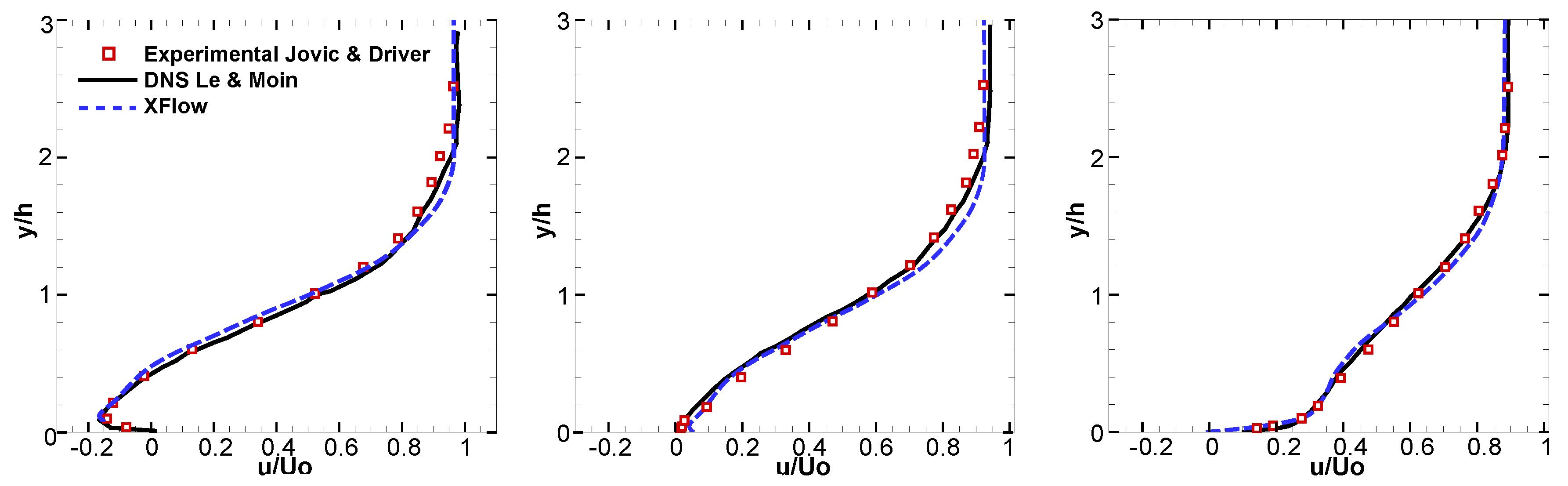
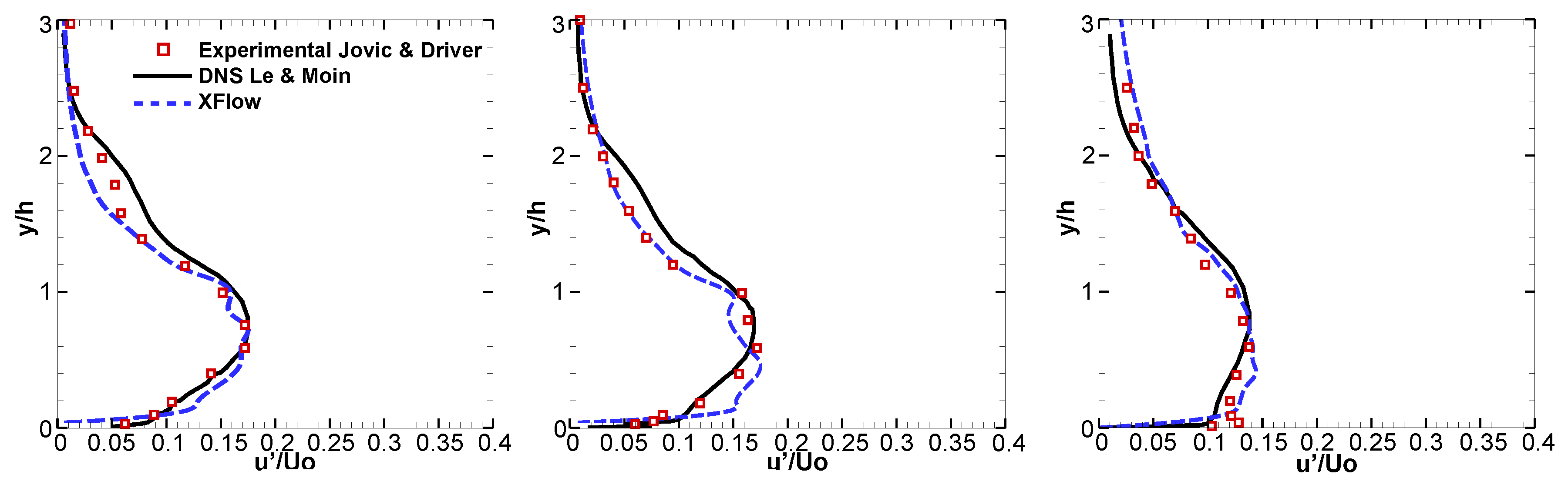
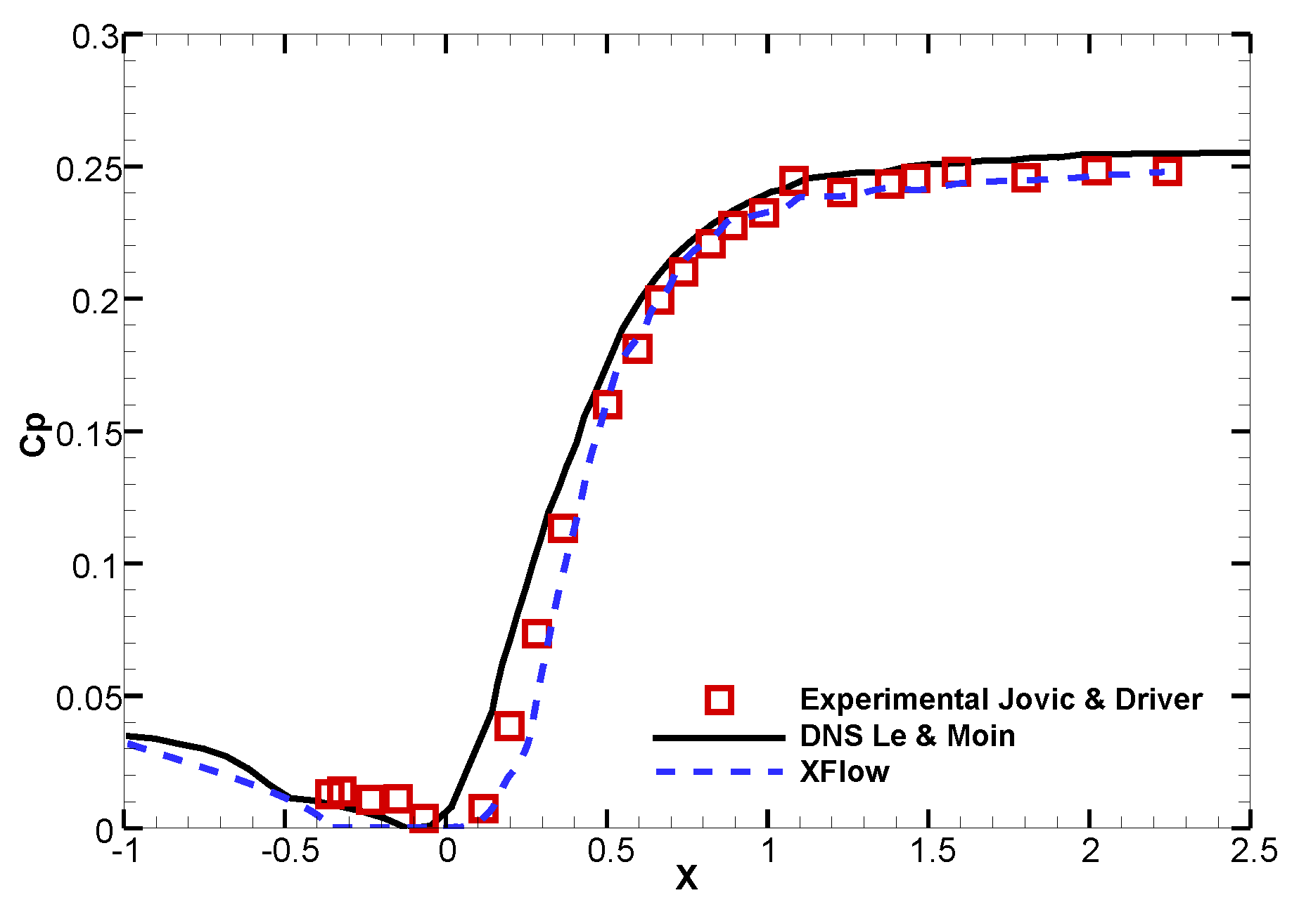
3.1. Backward-Facing Step

3.1.1. Introduction

The backward-facing step problem is a fundamental test case to validate reattached and separated flows. The phenomenon of flow separation is a problem of great importance for fundamental and industrial reasons. Armaly et al. [13] presented a detailed experiment on the backward-facing step geometry. According the Reynolds number, $R{e}_D=\frac{\rho UD}{\mu }$, the flow regime can be laminar or turbulent. Here $D=2h$ denotes the hydraulic diameter of the inlet channel with the step height, h.

The flow is laminar when the Reynolds number is $R{e}_D<400$ and it can be assumed to be a two-dimensional problem. Under these conditions a recirculation zone appears where a strong mixing process takes place. The flow becomes three-dimensional when the Reynolds number is $R{e}_D>400$. Furthermore, when the Reynolds number is round $R{e}_D$∼1200, the flow suffers a transition process from laminar to turbulent flow. The simulation is performed with Reynolds number $R{e}_h=5100$ [42], so that, the flow is strongly three-dimensional and turbulent.

3.1.2. Setup and Mesh Convergence

The setup simulation was set according to Le and Moin’s [43]. The computational domain (see Figure 5) is defined with the following dimensions: $L_x=30$ m (10 m prior to the step and a 20 h post-expansion section), $L_y=6$ m, $L_z=1.25$ m and $h=1$ m, giving an expansion ratio is $ER=L_y/(L_y-h)=1.2$.

Free slip boundary conditions were used at the top boundary and periodic boundaries were set for lateral walls. No-slip boundaries were used for the backward-facing step. A velocity inlet boundary condition was used at the inlet and a convective pressure outlet was imposed at the outlet. To simulate this case, a single phase external flow set up with the isothermal model wasselected. In addition, the turbulence model, Wall-Adapting Local Eddy-viscosity (WALE), was used. The reference velocity and length used to compute aerodynamic coefficients are $U_0=1$ m/s and $h=1$ m. The density and dynamic viscosity is selected as $\rho =1{\mathrm{Kg}/\mathrm{m}}^3$ and $\nu =1.96·{10}^{-4}\mathrm{Pa}·\mathrm{s}$, in order to obtain a Reynolds number $R{e}_h=5100$. At the inlet, a velocity profile is imposed and is defined by a Reynolds number $R{e}_{\theta }=670$ ($R{e}_{\delta \ast }=1000$), where $\theta$ is the momentum thickness and ${\delta }_{99}=6.1\delta \ast$ [44].

Grid independence is checked using four different grid sizes, as summarised in

Table 1. Grid independence with $R{e}_h=5100$.

	Lattice Resolution (mm)	Elements	Simulation Time (s)	${\mathit{X}}_{\mathit{r}}/\mathit{h}$	Comp. Time (h)	Cores
Coarse	78.1	$0.45·{10}^6$	0.5	9.16	0.3	8
Medium	58.6	$1.06·{10}^6$	0.5	7.42	0.8	8
Fine	48.8	$1.82·{10}^6$	0.5	6.81	2.1	8
Extra-Fine	38.8	$3.64·{10}^6$	0.5	6.33	3.5	8
Le and Moin [43]	-	$8.3·{10}^6$	-	6.28	-	-
Jovic and Driver [42]	-	-	-	6.00	-	-

. The reattachment length, $X_r$, is used for the convergence analysis. It is calculated in different positions in the spanwise direction and averaged the last 0.15 s of the simulation.

The reattachment length converges to a value $X_r=6.33h$, which is in good agreement with the reattachment length calculated by Le and Moin [43], $X_r=6.28h$ and obtained from experiment by Jovic and Driver [42], $X_r=6.00h$. Therefore, the Extra-Fine grid was retained in the following section.

3.1.3. Results

In addition to the reattachment length, included in Table 1, in this section we included the distribution of mean and standard deviations for the velocity and pressure at different longitudinal sections, $X/h$ = 4 (recirculation region), 6 (reattachment location) and 10. The results extracted from XFlow are compared with Le and Moin [43] and Jovic and Driver [42] numerical and experimental results, respectively.

Figure 6 shows the mean x-velocity profile at the three sections, $X/h=$ 4, 6 and 10. The figure shows very good agreement between XFlow and the DNS/experiments for the mean velocity. We observe a small region with flow acceleration near the recirculation at $X/h$ = 4, but the global trend is correct.

Turbulent fluctuations are compared in Figure 7 through the standard deviation profile in the x-direction. The numerical results show good agreement with the reference data.

Finally, Figure 8 shows the streamwise pressure coefficient defined as $Cp=\frac{p-p_{\infty }}{\frac{1}{2}\rho U_0^2}$. Again XFlow’s results agree well with the reference data.

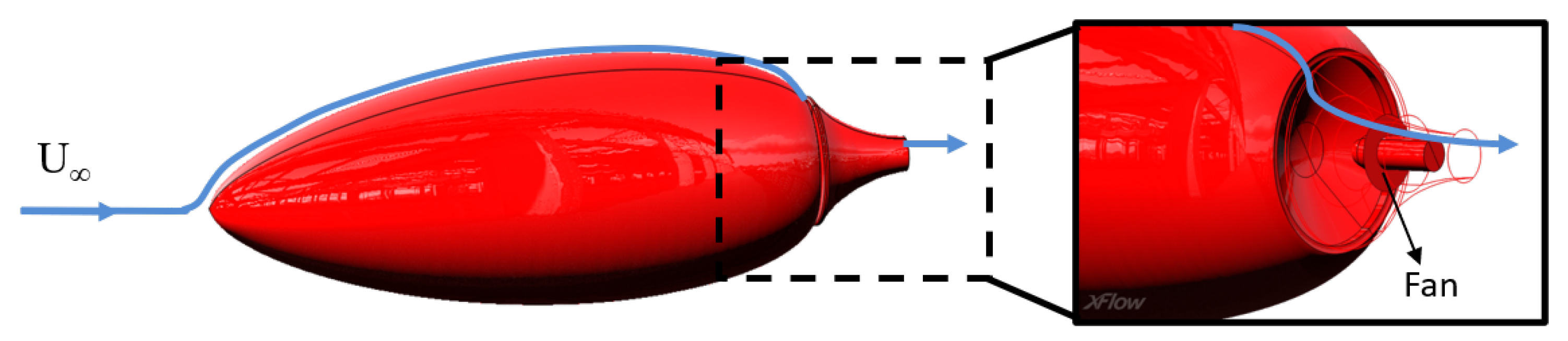
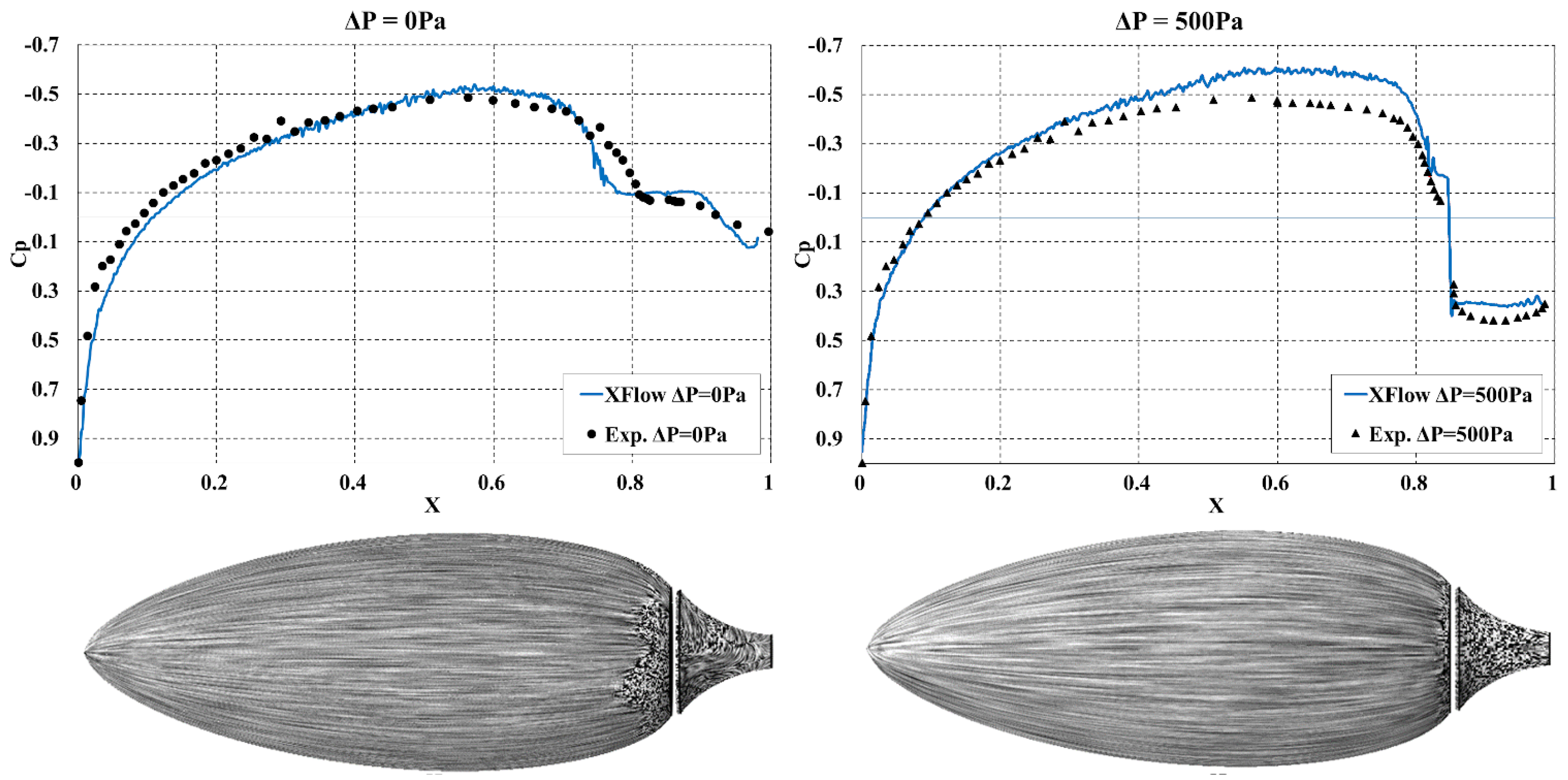
3.2. Goldschmied Body

3.2.1. Introduction

The self-propulsive fuselage concept was introduced by F. R. Goldschmied in the 50’s [14,45] showing promise in reducing drag and increasing the aerodynamic efficiency of bullet shape fuselages (see Figure 9). Namely, Goldschmied introduced the idea of including an almost passive flow control strategy to force the flow to remain attached, hence reducing drag. To control separation a fan is installed within the body tail and induces a pressure deficit. It is capable of forcing the flow to remain attached even in presence of strong adverse pressure gradients induced by the body geometry. The challenge for XFlow is to predict correctly the detached flow with different pressure gradients produced by the fan.

3.2.2. Setup and Mesh Convergence

The model was created from the Thomason’s work [45]. It was tested in a wind tunnel with the following dimensions: 12 m long, $1.22$ m wide and $0.9$ m height. The free slip boundary condition was used at the lateral walls. A velocity inlet boundary condition was used at the inlet and convective pressure outlet at the outlet. For the Goldschmied’s wall, the boundary condition of non-equilibrium wall function was imposed to take into account pressure gradients in separated regions. The fan boundary condition was imposed through a pressure gradient, $\Delta$P. To simulate this case, a single phase external flow set up with the isothermal model has been selected. In addition, Wall-Adapting Local Eddy-viscosity (WALE) turbulence model, was used.

The reference velocity and length used to compute aerodynamic coefficients are $U_{\infty }=20$ m/s and $S_{\mathrm{ref}}=0.2402{\mathrm{m}}^2$ (frontal surface area). The resulting Reynolds number (based on the free stream velocity and the body area) is Re $=8.9·{10}^4$.

In reference to the grid dependency, three different grid sizes for the zero pressure gradient condition, $\Delta \mathrm{P}=0$ Pa, were computed, as shown

Table 2. Grid independence at $\Delta \mathrm{P}=0$ Pa.

	Lattice Resolution (mm)	Elements	Simulation Time (s)	Cd	Comp. Time (h)	Cores
Coarse	4	$1.3·{10}^6$	0.5	0.24	3.2	16
Medium	2	$6.5·{10}^6$	0.5	0.091	10	32
Fine	1.5	$30.3·{10}^6$	0.5	0.066	25	64
Experimental	-	-	-	0.055	-	-

. The mean drag coefficient, Cd, is computed over the last 0.1 s of the simulation and converges towards the experimental value when refining the mesh. Therefore, the Fine grid was used for the following simulations because it has a better agreement between the simulations and experimental values. An adaptive grid refinement in function of the vorticity field was used during the computations.

3.2.3. Results

Additionally to the Cd comparison shown in Table 2, Figure 10 shows the pressure coefficient distribution and surface flow pattern for both pressure gradient condition, $\Delta \mathrm{P}=0\mathrm{Pa}$ and $500\mathrm{Pa}$, with the finest grid. When comparing these distributions against experimental values it appears that the numerical solution predicts accurately the detached flow position. For $\Delta \mathrm{P}=0\mathrm{Pa}$, detachment occurs slightly before than in the experiments; however the pressure drop level is well behaved. When the cotrol is activated, at $\Delta \mathrm{P}=500\mathrm{Pa}$, the pressure coefficient is slightly over predicted; however the detachment flow point is well captured.

3.3. 2nd High-Lift Prediction Workshop

3.3.1. Introduction

The 2nd High-Lift Prediction Workshop (HiLiftPW-2) [6,15] provides a benchmark to study linear and post-stall regions on a high-lift aircraft configuration. The DLR F11 geometry includes geometrical details such as slat tracks, flap track fairings and slat pressure tube bundles, which introduce complexity when generating the mesh.

This section contains part of the results published by Holman et al. [6] with the most complex geometry. They focused on the linear region of lift, drag and moments curves, and pressure coefficient distributions. However, only a few participants were able to predict the stall and the post-stall regions [46] produced by the slat tracks, flap track fairings and tubes bundle.

3.3.2. Setup and Mesh Convergence

The geometry is based on the DLR F11. The study employs the Configuration 2 is formed by a wing (with deflected slat and flap, with $26.5$ deg and 32 deg respectively) and fuselage. Configuration 5 is based on Configuration 2 geometry including slat tracks, flap track fairings, and pressure tube bundles, as shown in Figure 11a). The reference area for dimensioning the aerodynamic coefficient is $S_{\mathrm{ref}}=0.41913{\mathrm{m}}^2$ and the moment reference center is $x=1.4289\mathrm{m}$, $y=0.0\mathrm{m}$, and $z=-0.04161\mathrm{m}$.

The simulation is set in the XFlow environment, which features a virtual wind tunnel. The virtual wind tunnel defines a rectangular domain with pre-set boundary conditions designed for external aerodynamics. In this case, the wind tunnel size is ($40,20,20$) m, which is wide enough to avoid significant wall and blockage effects. The boundary conditions are set as an inlet velocity with $59.5$ m/s, which corresponds to a Mach number of $0.175$, and an outlet boundary set as gauge pressure outlet of zero Pascals to mimic atmospheric conditions. The symmetry plane is set as a free-slip ground wall.

Experimental data with two different flow conditions was provided by the HiLiftPW-2 committee. Two Reynolds number were defined, Re $=1.35·{10}^6$ and $15.1·{10}^6$ and the Mach number was set to Ma $=0.175$, for both Reynolds. Here, we only present the results for the higher Reynolds number (Re $=15.1·{10}^6$). The solver is set as single-phase, isothermal and the WALE turbulence model is selected. The velocity field is initialized with the magnitude and direction of the input boundary, and the initial pressure field is set to zero within the entire fluid domain.

We perform a grid convergence study to determine the spatial discretization required to capture the physics appropriately. The HiLiftPW-2 committee provided coarse, medium, fine and extra-fine meshes, for the participants to run their codes and to check convergence. However, XFlow avoids the traditional meshing process using an octree structure to address any complex geometry.

Comparisons for different sizes of near-wall refinements (extra-coarse, coarse, medium, and fine resolutions) are included in

Table 3. Grid independence at 16 deg.

Grid	Fuselage (mm)	Wing (mm)	Elements	Sim. Time (s)	Cd	Cl	Comp. Time (h)	Cores
Extra-Coarse	4	4	$9.2·{10}^6$	0.1	0.262	1.95	160
Coarse	2	2	$25.9·{10}^6$	0.1	0.295	2.16	5.2	160
Medium	1	1	$87.4·{10}^6$	0.1	0.296	2.51	33.8	160
Fine	2	0.5	$150·{10}^6$	0.1	0.310	2.67	84	256
Experimental	-	-	-	-	0.275	2.68	-	-

at $\alpha =16$ deg. These meshes use the farfield scale fixed to $0.256$ m, using the Configuration 2. The criterion of convergence is based on the global lift and drag coefficients, averaged for the last 0.02 s of the simulation. We can clearly observe that the solution improves when the lattice is refined near the aircraft walls. Namely, the extra-fine grid provides good accuracy, showing a relative error, for the lift prediction (in comparison with wind tunnel), of only $0.4\%$, at 16 deg. However, note that coarser meshes also provide accurate drag coefficients with a lower number of lattices.

An important influence to the lattice resolution near walls is observed. However, the drag and lift are well captured once a resolution of $0.5$ mm on the wing is set. The fine resolution provides a good accuracy with an acceptable computational time, and is therefore retained for the rest of the study.

3.3.3. Results

In this section, we report Xflow results, which are compared to experimental data, for the aerodynamic coefficients, including a full polar curve. Figure 11a shows the lift coefficient for both configurations which agrees well to the experimental data below 16 deg, in the linear region, where both absolute lift value and linear lift slope are successfully predicted. For example, the lift coefficient predicted at 16 deg by XFlow shows a relative error of only $0.7$% when compared to wind-tunnel data, and the linear slope is exactly matched. Additionally, we observe that the track fairings and the pressure tube bundles have a negligible effect on the aerodynamics, in the linear region. Differences appear near stall, where the stall angle of attack is predicted at $22.4$ deg in XFlow, while it is 21 deg for the wind-tunnel data. We observe that when including the the flap track fairings, slat tracks and slat pressure tube bundles, the coefficient change significantly in this region, suggesting a high sensitivity of the aerodynamics to these geometric components, near stall.

Additionally, XFlow predicts very well the experimental flow topology, as depicted in Figure 11b, where the WMLES turbulence modeling can be appreciated. The flow structure at 24 deg can be observed in Figure 11c, which compares the two configurations. The figure shows the generation of turbulent strips in conf. 5, which is induced by the slat tracks and the slat pressure tube bundles. This turbulent pattern is not visible in conf. 2.

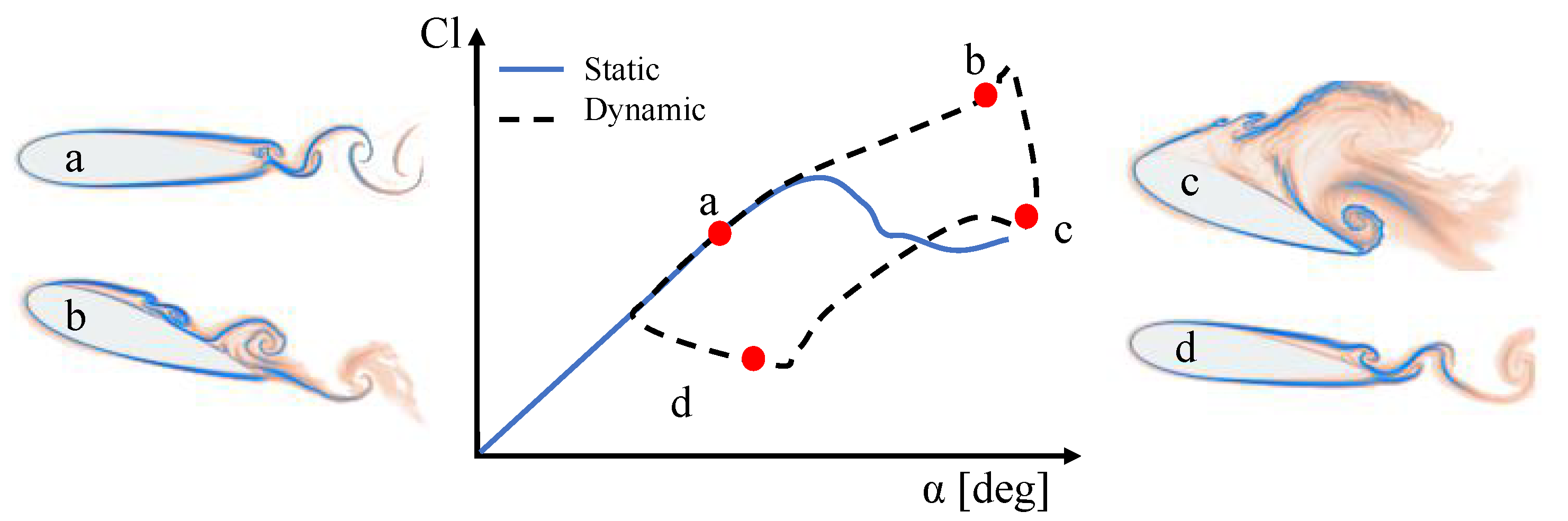
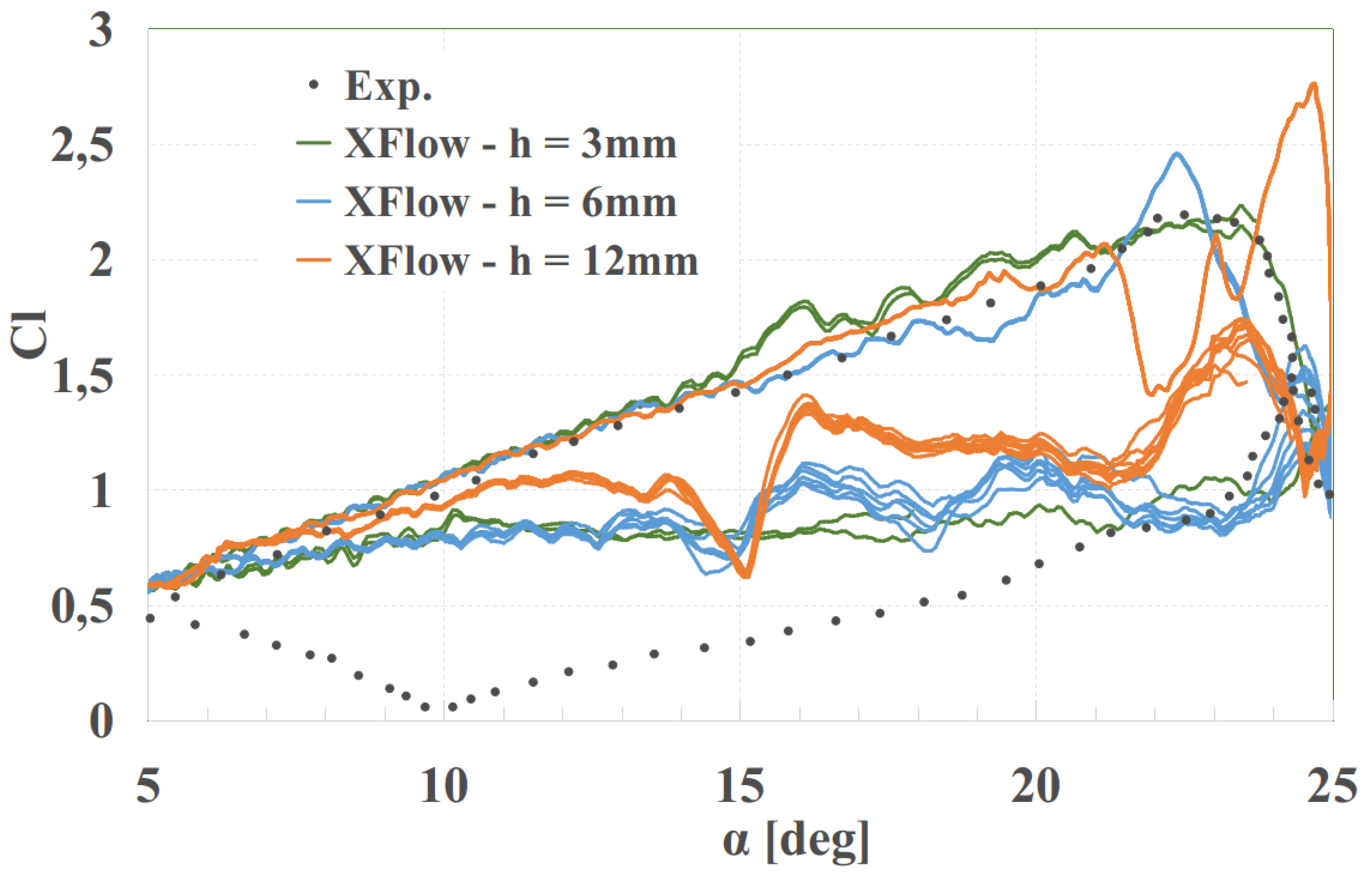
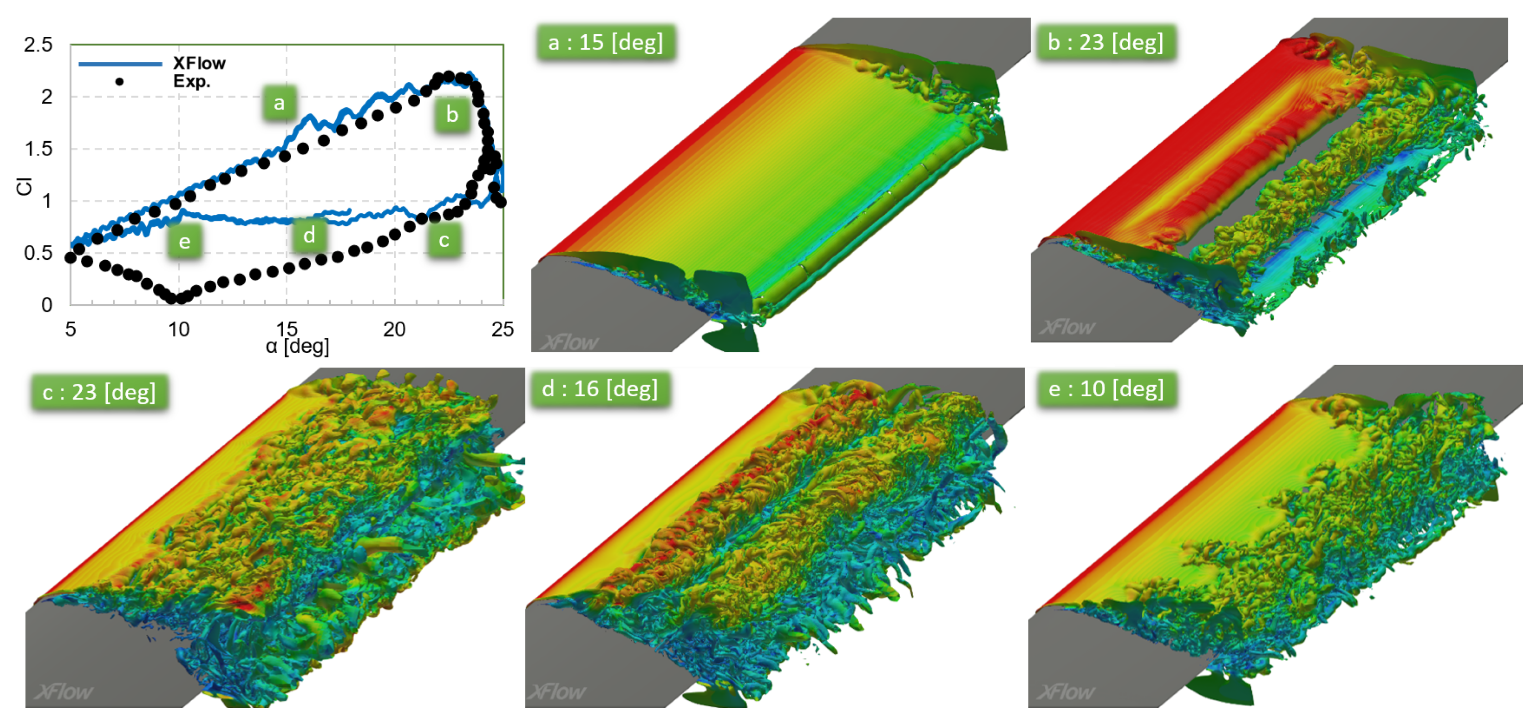
3.4. Dynamic Stall: NACA0012

3.4.1. Introduction

The symmetric airfoil NACA0012 was selected to validate XFlow when computing flows around moving geometries. The main aerodynamic differences between static and rotating lift curves are sketched in Figure 12. Dynamic stall occurs when a rapid variation in the angle of attack is seen by the airfoil and typically leads to a hysteresis cycle in the aerodynamic forces. It is related to the apparition of a vortex near the leading edge on the suction side that enhances lift considerably (when compared to the static case). Massive and abrupt stall, linked to a sudden loss of lift, occurs once the vortex convects at the trailing edge. This phenomenon was widely studied experimentally and numerically due to its appearance in helicopters aerodynamics and wind turbines [16,47,48,49].

The variation of the angle of attack, $\alpha$ in the dynamic simulation is described by the following equation:

$$\alpha ={\alpha }_0+{\alpha }_{\mathrm{amp}}sin\omega t\mathrm{with}\omega =\frac{2U_{\infty }k}{c},$$

(9)

where ${\alpha }_0$ is the initial angle of attack, ${\alpha }_{amp}$ is the angle of attack amplitude, $\omega$ is the pitch rate, $U_{\infty }$ is the reference velocity, k is the reduced frequency and c the reference chord length.

It is interesting to note that the pitch rate, $\omega$, is directly governed by the non-dimensional reduced frequency, k. The reduced frequency governs the degree of unsteadiness such that for steady state aerodynamics $k=0$, quasi-steady aerodynamics, $0\le k\le 0.05$, and unsteady aerodynamics, $k>0.05$. Additionally, for $k>0.2$ it is considered highly unsteady aerodynamics [16]. In this study, a rotational velocity, $k=0.1$ was chosen to show the capability of XFlow to predict the dynamic stall. Lift, drag and pitching moment will be compared to experimental data [16].

3.4.2. Setup and Mesh Convergence

The geometry for this study corresponds to the well-known NACA0012 airfoil. The reference chord length is $c=0.61$ m (or aerodynamic chord). The center of rotation is located at 25% of reference length, c, from the leading edge. These reference values are used to calculate the lift and drag coefficients and the pitching moment coefficient respectively.

A rectangular domain was used with $32c$ long, $5c$ height and $2.5c$ wide. Farfield velocity boundary condition is used at the inlet and zero gauge pressure at the outlet. For the lateral walls, slip walls were used. At airfoil walls, non-equilibrium wall function is selected to take into account pressure gradients that may govern separation and stall. Additionally, the rotating geometry is addressed with immersed boundary method. An external flow (single phase and air fluid properties) with the isothermal flow condition and the turbulence model, Wall-Adapting Local Eddy-viscosity (WALE). Where flow conditions are defined through the non-dimensional numbers: Mach number, Ma $=0.072$, Reynolds number, Re $=0.98·{10}^6$, and reduced frequency, $k=0.1$.

In reference with the grid refinement, Figure 13 shows the grid convergence for different refinements (see

Table 4. Grid independence with k = 0.1.

	Lattice Resolution (mm)	Elements	Simulation Time (s)	Comp. Time (h)	Cores
Coarse	12	$0.3·{10}^6$	2	3.8	8
Medium	6	$1.4·{10}^6$	2	24.5	8
Fine	3	$9.5·{10}^6$	2	100	40

). Figure 13 depicts the hysteresis for all lattice sizes. Additionally, we observe that for the finest mesh, the linear region and the maximum lift are well captured. Discrepancies can be seen in the low part of the curve, for all mesh sizes.

3.4.3. Results

In this section, the lift coefficient hysteresis and snapshots during the dynamic simulation with the Fine grid are shown in Figure 14. The lift coefficient was compared with experimental data [16].

XFlow captures well the maximum lift. The hysteresis is relatively well captured although discrepancies are observed in the recovery region. The instantaneous vorticity iso-countours are depicted for various angles of attack, which correspond to different points in the lift hysteresis loop. Please note that in the linear region, the flow is mainly attached (see Figure 14a). In Figure 14b the flow detached and the convective vortex characteristic of rapid pitching (and dynamic stall) is near the end of the wing, which will soon produce an abrupt stall. The snapshots are consistent with the simulated and experimental curve. Figure 14c is characterized by massive detachment and deep stall, the suction side of the wing shows indeed massive detachment. The lift coefficient in Figure 14d,e disagrees between computations and experiments. In these regions XFlow predict a more rapid recovery (less detachment) that in the experiments.

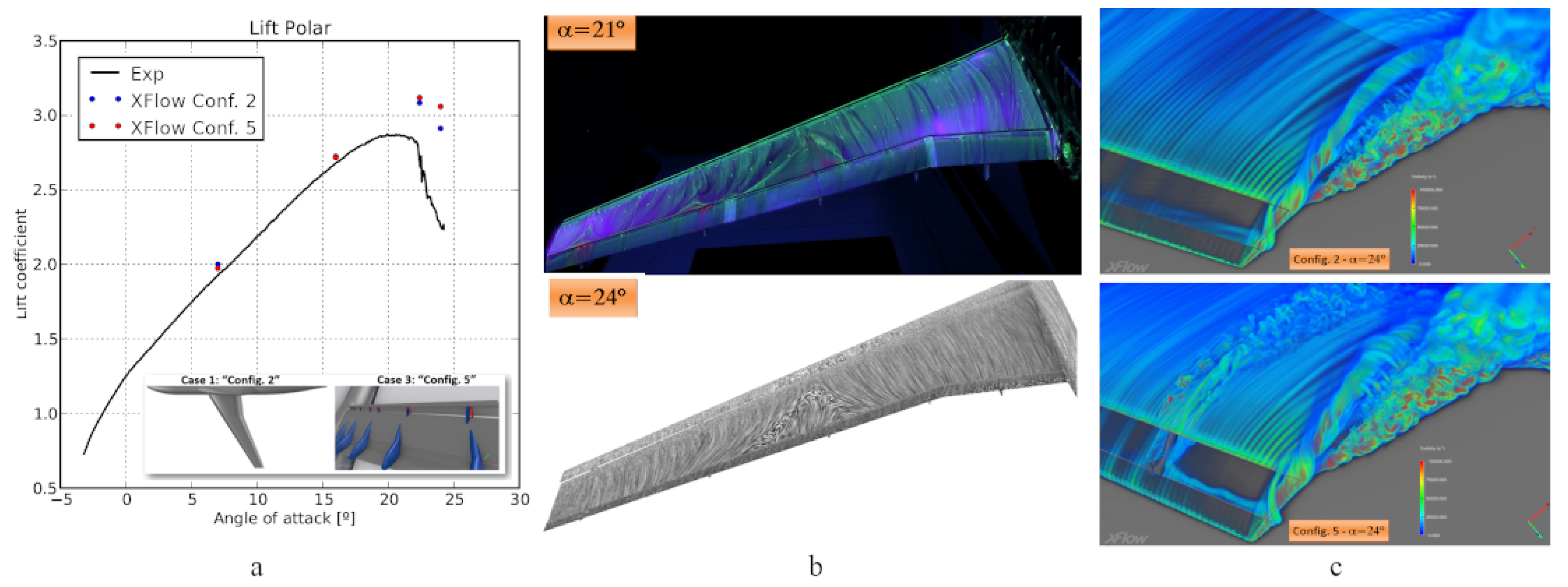
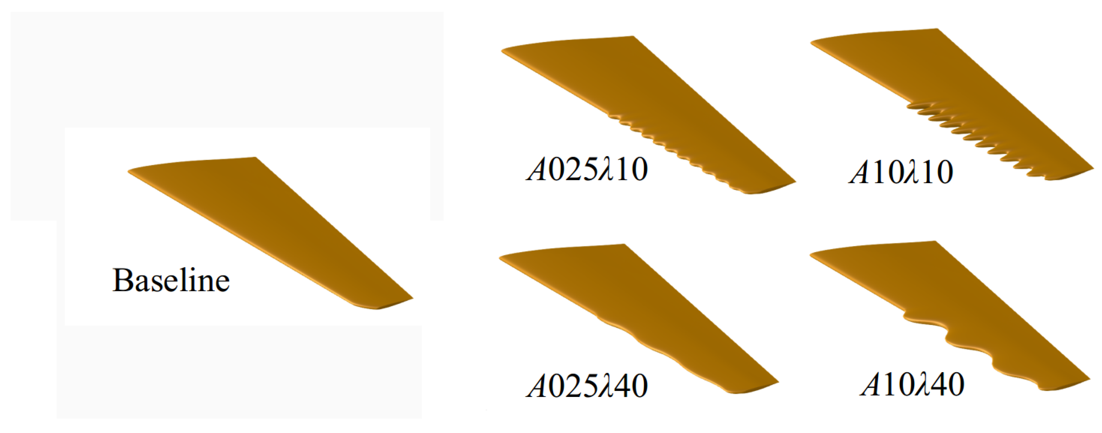
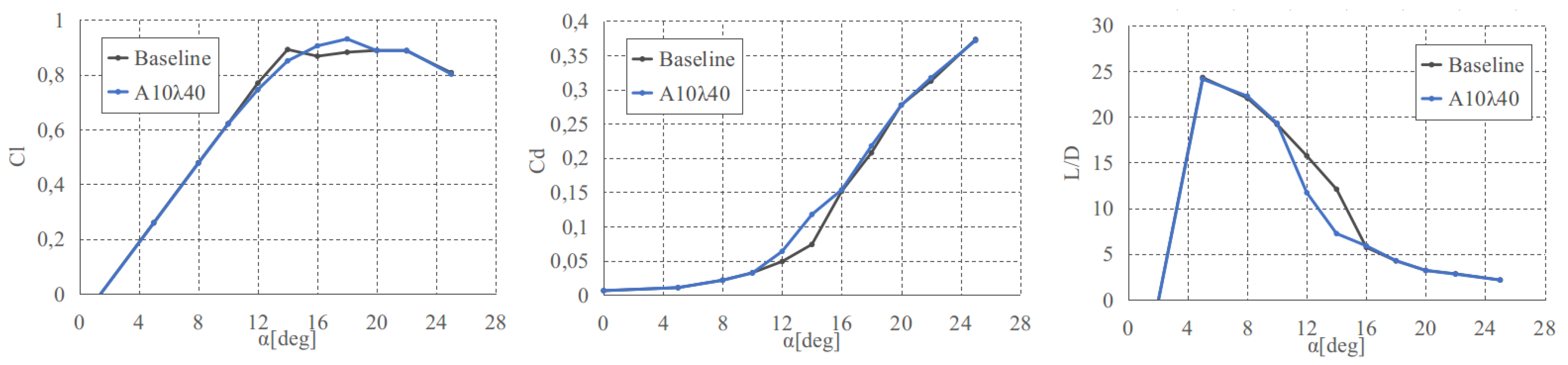
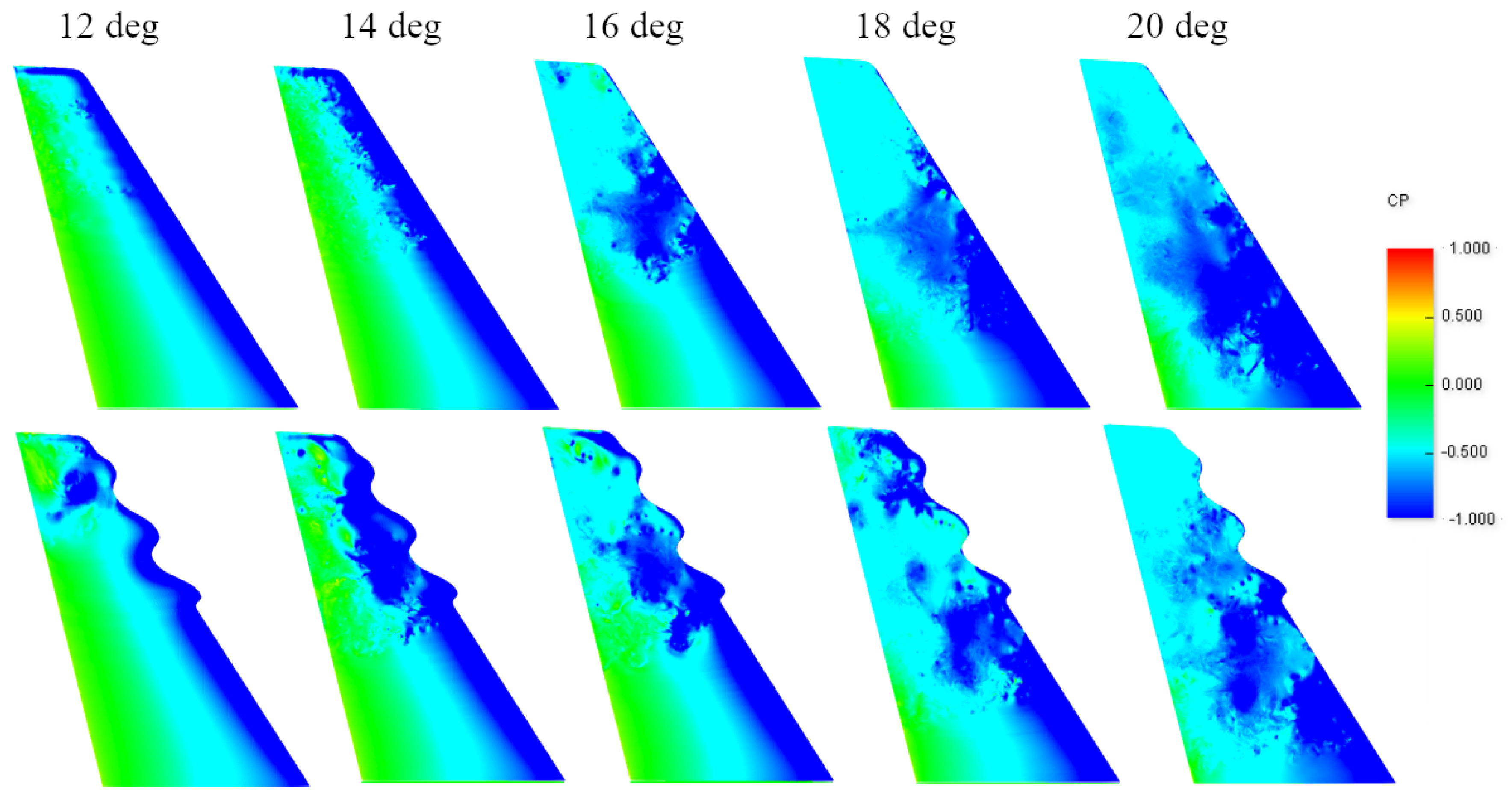
3.5. Wing with Leading-Edge Tubercles

3.5.1. Introduction

Tubercles were proposed to soften aerodynamic characteristics near stall, the origin of this idea goes back to Humpback whale’s fins [17] (see Figure 15), which evolved during millions of years of evolution to enhance manoeuvrability in water. For example, an amazing feature of the humpback is its acrobatic behavior during feeding known as bubble netting. These whale’s fins operate at Reynolds numbers, Re $=1.1·{10}^6$, based on the sea water viscosity and density at 16 ${}^{\circ }$C.

Tubercles are among other passive flow control devices, being explored to enhance aerodynamic performance. An overview of devices that may help control stall or improve performance (decrease drag) was summarized by Aftab et al. [50]. The geometrical parameters that define the tubercles are the following:

• Wavelength, $\lambda /c$: defines the non-dimensional wavelength (or equivalently the spatial frequency) of the tubercles, with c being the local chord.
• Amplitude, $A/c$: defines the amplitude of the tubercles. It is also made non-dimensional using the local chord c.
• Span section, $\eta /b$: defines the wing span section where the tubercles start. Please note that b is the total wing span.

Aerodynamic characteristics at different Reynolds were obtained in experiments. Johari et al. [51] tested a NACA63${}_4$021 airfoil, at angle of attack range from 6 deg to 30 deg and Re $=1.83·{10}^5$ and $2·{10}^6$. Airfoils with varying tubercle amplitude, $A=0.025c,0.05c$ and $0.12c$ and wavelength $\lambda =0.25c$ and $0.5c$ were tested [52]. Forces and moments were measured in a water tunnel. The results showed smooth stall, due to the presence of the tubercles, improving the post-stall behavior by $50\%$. Configurations with small amplitude, $A=0.025c$, and large wavenumber $\lambda =0.5c$ gave better results. Additionally, tubercles provide a reduction in performance in the pre-stall region but avoid the abrupt stall noticed for the baseline airfoil. Later, Wei et al. [53] reported the differences between directing the tubercles normal to the span (modified A) or normal to the tapered leading edge (modified B). These also considered a tapered wing with sweep-back, with tubercles of amplitude, $A=0.12c$, where c is the mean chord for rectangular wing and larger wavelength, $\lambda =0.5c$. Johari et al. obtained similar results with these configurations where the post-stall behavior improve; however the drag increased slightly. In this section, a swept-wing is used to study the effect of the tubercles leading-edge in the aerodynamic properties.

3.5.2. Setup and Mesh Convergence

A swept-wing geometry was used for this study. The analysis was performed using a baseline geometry, which was modified to include tubercles configurations. The mean aerodynamic chord and the wingspan are MAC $=2.702$ m and $b=6.225$ m respectively. The wing with leading-edge tubercles was based on the baseline wing.

In this study, the tubercles were varied to study their effect over the aerodynamic coefficients. The parametric study was defined with the frequencies $\lambda /c=0.1,0.2$ and $0.4$, and the amplitudes $A/c=0.025,0.05$ and $0.1$. These values were selected based on previous studies by Wei et al. [53], who showed that for these values, the effect of the tubercles were more noticeable in this type of wing configuration.

Table 5. Configurations of leading-edge tubercles with leading edge tubercles of varying amplitude and frequency.

Baseline		$\mathit{c}=$ 2.702 m	$\mathit{b}=$ 6.225 m
	$\mathit{A}/\mathit{c}$	0.025	0.05	0.1
$\mathit{\lambda }/\mathit{c}$
0.1		A025$\lambda$10	A05$\lambda$10	A10$\lambda$10
0.2		A025$\lambda$20	A05$\lambda$20	A10$\lambda$20
0.4		A025$\lambda$40	A05$\lambda$40	A10$\lambda$40

shows the different set of parameter used to generate 9 different tubercles configurations. Additionally, the idea was to localize the tubercles only near the wing tip, since the baseline wing geometry was observed that stall initiates at the tip, in this study fixed to $\eta /b=0.50$. Selected configurations are shown in Figure 16.

The wind tunnel dimensions for the simulation are: $37c$ long, $9.25c$ wide and $18.5c$ height. The symmetry wall was defined as free slip wall where the wing geometry relies on it. Velocity inlet boundary conditions are used at the inlet. Zero-gauge pressure is imposed at the outlet. Finally, the wing wall required the non-equilibrium enhanced wall functions to take into account pressure gradients. An external flow (single phase and air fluid properties) with the isothermal flow condition and the turbulence model: Wall-Adapting Local Eddy-viscosity (WALE) were selected.

The flow condition is defined by the Mach number which is set to Ma $=0.2$ and the Reynolds number was fixed to $\mathrm{Re}/L=4.66·{10}^6$ with a reference length, L. The latter Mach and Reynolds correspond to see level conditions. Please note that for each new geometry the surface area was computed. This area is then used to non-dimensionalize the lift and drag forces, such that the resulting aerodynamic coefficients are consistent and represent the relative force to the modified shape.

The wing with $A/c=0.025$ and $\lambda /c=0.2$ was used to study mesh convergence. For this purpose, we select an angle of attack, $\alpha =18$ deg. It corresponds to the stall region in the lift curve (as will be shown later in Figure 17). To ensure that the mesh refinement does not affect the results, a comparison was performed for different sizes of near wall refinements. In all cases the farfield scale is 5.12 m.

Table 6. Grid independence with configuration $A/c=0.025$ and $\lambda /c=0.2$ at $\alpha =$ 18 deg.

	Lattice Resolution (mm)	Elements	Simulation Time (s)	Cd	Cl	Comp. Time (h)	Cores
Extra Coarse	40	$3.3·{10}^6$	3	0.254	0.780	19	8
Coarse	20	$4.2·{10}^6$	3	0.242	0.872	28	8
Medium	10	$12.3·{10}^6$	3	0.218	0.930	25	32
Fine	5	$42.0·{10}^6$	3	0.215	0.941	155	32

summarizes the lattice resolution, number of lattices in each grid, the drag and lift coefficients averaged the last 1s of the simulation, the computational time and the number of cores used for computation. The four simulations use adaptive mesh refinement based on the vorticity field with the lattice resolution value.

Regarding the lift and drag coefficients in Table 6, it can be seen that the errors between both resolution 5 and 10 mm are 1% for lift and 2% of drag. These convergence study is remarkable since at this angle of attack (with stalled flow), the flow is more complex to resolve. Looking for a trade-off between accuracy and computational cost, 10mm resolution (Medium mesh) was used for the rest of simulations.

3.5.3. Results

The results for lift, drag and efficiency at $\alpha =18$ deg are compared in

Table 7. Percentage variation of lift, drag and efficiency of the modified geometries (see Table 4) with respect to the baseline configuration.

	Baseline	$\mathit{A}10\mathit{\lambda }10$	$\mathit{A}05\mathit{\lambda }10$	$\mathit{A}025\mathit{\lambda }10$	$\mathit{A}10\mathit{\lambda }20$	$\mathit{A}05\mathit{\lambda }20$	$\mathit{A}025\mathit{\lambda }20$	$\mathit{A}10\mathit{\lambda }40$	$\mathit{A}05\mathit{\lambda }40$	$\mathit{A}025\mathit{\lambda }40$
$\Delta$Cd [%]	0	−8.3	−4.9	−3.5	−4.9	−2.6	−1.8	−1.7	2.8	−1.9
$\Delta$Cl [%]	0	−2.0	0.1	−1.7	0.4	0.0	0.1	4.1	5.5	0.8
$\Delta$L/D [%]	0	6.8	5.2	1.8	5.5	2.7	2.0	5.9	2.7	2.7

for all configurations. The percentages, indicate the percentage variation of the modified geometry with respect to the baseline configuration. First, it can be seen that variations are relatively small in general. Second, we observe that the configurations $A10\lambda 40$ and $A05\lambda 40$ show a more important increase in the lift coefficient. The $A05\lambda 40$ configuration shows an increase in the drag coefficient; however $A10\lambda 40$ shows a decrease in the drag coefficient. This can be further quantified by comparing the lift over drag, L/D, where they have a $5.9\%$ and $2.7\%$ gain in $L/D$ with respect to the baseline configuration. It may be concluded that $\lambda /c=0.4$ is the wavelength that provides the more benefit in terms of lift coefficient, and that amplitudes around $A/c=0.1$ show the most potential. In this work, the choice of the optimal configuration is based on $\Delta$Cd$[\%]<0$$\Delta$Cl$[\%]>0$ and with maximum $\Delta$L/D [%]. Therefore, the optimal tubercles configuration geometry is $A10\lambda 40$ ($A/c=0.1$ and $\lambda /c=0.4$).

Having determined the most promising configuration for a high angle of attack ($\alpha =18$ deg), the rest angles of attack were simulated as depicted in Figure 17. The baseline geometry was compared to the optimal tubercles configuration geometry ($A/c=0.1$ and $\lambda /c=0.4$). More interestingly, note that the geometries with tubercles show an identical lineal regime for low angle of attack and a higher maximum lift with a more benign stall. However, when comparing the drag, we observe a mild increase at medium range of angles of attack that results in a decrease of the L/D. Overall, the efficiency, L/D, shows that the tubercles diminish the performance at medium range angles of attack, even if the lift coefficient improves near stall. These trends are remarkably similar to the experiments reported in Wei Wei et al. [53] for a tapered swept-back wing, which was mentioned in the introduction of this section.

For completeness, Figure 18 includes visualization of instantaneous pressure contours on the wing surface for various angles of attack. The figures suggest that the higher lift at large angles of attack is related to localized suction regions, which are generated by the tubercles. These regions are particularly present at angles 12, 14 and 18 deg and located near the wing tip. These results suggest that acting on the wing tip may have a beneficial effect on the aerodynamic performance, perhaps more important that including tubercles along $50\%$ of the span.

4. Conclusions

This work showed that the lattice Boltzmann method implemented in XFlow is able to solve advanced flow problems even in the presence of complex geometries or moving parts. Five industrial cases were studied, showing the reliability of the lattice Boltzmann method to resolve detached flows in engineering problems of industrial interest.

The automation of the the generation using octrees for any geometry and angle of attack in XFlow, shortened significantly the setup of the simulation included, which transforms most engineering efforts into machine cost. Mesh automation using octrees does not damage the accuracy of accurate results, that agree well with published data for detached flows. Furthermore, the simulations were run in competitive turnaround times, even when using an unsteady LES approach. It is concluded that XFlow provides accurate results for detached flows enabling the study of the stall flows, where the flow becomes highly unsteady and turbulent, while minimising human interactions.

References

1. Vincent, P.E.; Jameson, A. Facilitating the adoption of unstructured high-order methods amongst a wider community of fluid dynamicists. Math. Model. Nat. Phenom. 2011, 6, 97–140. [Google Scholar] [CrossRef]
2. Allahyari, M.; Esfahanian, V.; Yousefi, K. The Effects of Grid Accuracy on Flow Simulations: A Numerical Assessment. Fluids 2020, 5, 110. [Google Scholar] [CrossRef]
3. Patankar, S.V.; Spalding, D.B. A calculation procedure for heat, mass and momentum transfer in three-dimensional parabolic flows. In Numerical Prediction of Flow, Heat Transfer, Turbulence and Combustion; Elsevier: Amsterdam, The Netherlands, 1983; pp. 54–73. [Google Scholar]
4. Jacqmin, D. Calculation of two-phase Navier–Stokes flows using phase-field modeling. J. Comput. Phys. 1999, 155, 96–127. [Google Scholar] [CrossRef]
5. Allahyari, M.; Mohseni, K. Numerical simulation of flows with shocks and turbulence using observable methodology. In Proceedings of the 2018 AIAA Aerospace Sciences Meeting, Kissimmee, FL, USA, 8–12 January 2018; p. 0066. [Google Scholar]
6. Holman, D.M.; Brionnaud, R.M.; Chávez-Modena, M.; Sánchez, E.V. Lattice Boltzmann method contribution to the second high-lift prediction workshop. J. Aircr. 2015, 52, 1122–1135. [Google Scholar] [CrossRef]
7. Brionnaud, R.; Chávez Modena, M.; Trapani, G.; Holman, M.D. Direct noise computation with a Lattice-Boltzmann method and application to industrial test cases. In Proceedings of the 22nd AIAA/CEAS Aeroacoustics Conference, Lyon, France, 30 May–1 June 2016; p. 2969. [Google Scholar]
8. Sanders, L.; Manoha, E.; Murayama, M.; Yokokawa, Y.; Yamamoto, K.; Hirai, T. Lattice-Boltzmann flow simulation of a two-wheel landing gear. In Proceedings of the 22nd AIAA/CEAS Aeroacoustics Conference, Lyon, France, 30 May–1 June 2016; p. 2767. [Google Scholar]
9. Trapani, G.; Brionnaud, R.; Holman, D. XFlow contribution to the third high-lift prediction workshop. In Proceedings of the 2018 Applied Aerodynamics Conference, Atlanta, GA, USA, 25–29 June 2018; p. 2847. [Google Scholar]
10. Thibault, S.; Holman, D.; Garcia, S.; Trapani, G. CFD Simulation of a quad-rotor UAV with rotors in motion explicitly modeled using an LBM approach with adaptive refinement. In Proceedings of the 55th AIAA Aerospace Sciences Meeting, Grapevine, TX, USA, 9–13 January 2017; p. 0583. [Google Scholar]
11. Grondeau, M.; Guillou, S.; Mercier, P.; Poizot, E. Wake of a Ducted Vertical Axis Tidal Turbine in Turbulent Flows, LBM Actuator-Line Approach. Energies 2019, 12, 4273. [Google Scholar] [CrossRef] [Green Version]
12. Trapani, G.; Brionnaud, R.M.; Holman, D.M. Non-linear fluid-structure interaction using a partitioned lattice Boltzmann-FEA approach. In Proceedings of the 46th AIAA Fluid Dynamics Conference, Washington, DC, USA, 13–17 June 2016; p. 3636. [Google Scholar]
13. Armaly, B.F.; Durst, F.; Pereira, J.; Schönung, B. Experimental and theoretical investigation of backward-facing step flow. J. Fluid Mech. 1983, 127, 473–496. [Google Scholar] [CrossRef]
14. Goldschmied, F.R. On the aerodynamic optimization of mini-RPV and small GA aircraft. In Proceedings of the 2nd American Institute of Aeronautics and Astronautics, Applied Aerodynamics Conference, Seattle, WA, USA, 21–23 August 1984; Volume 21. [Google Scholar]
15. Rudnik, R.; Huber, K.; Melber-Wilkending, S. EUROLIFT test case description for the 2nd high lift prediction workshop. In Proceedings of the 30th AIAA Applied Aerodynamics Conference, New Orleans, LA, USA, 25–28 June 2012; p. 2924. [Google Scholar]
16. McCroskey, W.J.; McAlister, K.W.; Carr, L.W.; Pucci, S. An Experimental Study of Dynamic Stall on Advanced Airfoil Sections; Technical Report; Volume 1: Summary of the Experiment; NASA: Washington, DC, USA, 1982. [Google Scholar]
17. Miklosovic, D.; Murray, M.; Howle, L.; Fish, F. Leading-edge tubercles delay stall on humpback whale (Megaptera novaeangliae) flippers. Phys. Fluids 2004, 16, L39–L42. [Google Scholar] [CrossRef] [Green Version]
18. Boltzmann, L. Weitere studien über das wärmegleichgewicht unter gasmolekülen. In Kinetische Theorie II; Springer: Berlin/Heidelberg, Germany, 1970; pp. 115–225. [Google Scholar]
19. Premnath, K.N.; Banerjee, S. Incorporating forcing terms in cascaded Lattice Boltzmann approach by method of central moments. Phys. Rev. E 2009, 80, 036702. [Google Scholar] [CrossRef] [Green Version]
20. Chávez-Modena, M.; Ferrer, E.; Rubio, G. Improving the stability of multiple-relaxation lattice Boltzmann methods with central moments. Comput. Fluids 2018, 172, 397–409. [Google Scholar] [CrossRef]
21. Coreixas, C.; Chopard, B.; Latt, J. Comprehensive comparison of collision models in the lattice Boltzmann framework: Theoretical investigations. Phys. Rev. E 2019, 100, 033305. [Google Scholar] [CrossRef] [Green Version]
22. Geier, M.; Greiner, A.; Korvink, J.G. Bubble functions for the lattice Boltzmann method and their application to grid refinement. Eur. Phys. J. Spec. Top. 2009, 171, 173–179. [Google Scholar] [CrossRef]
23. Imamura, T.; Suzuki, K.; Nakamura, T.; Yoshida, M. Acceleration of steady-state lattice Boltzmann simulations on non-uniform mesh using local time step method. J. Comput. Phys. 2005, 202, 645–663. [Google Scholar] [CrossRef]
24. Arnone, A.; Liou, M.S.; Povinelli, L.A. Integration of Navier-Stokes equations using dual time stepping and a multigrid method. AIAA J. 1995, 33, 985–990. [Google Scholar] [CrossRef]
25. Bhaskaran, R.; Lele, S.K. Large eddy simulation of free-stream turbulence effects on heat transfer to a high-pressure turbine cascade. J. Turbul. 2010, 11, N6. [Google Scholar] [CrossRef]
26. Gardner, M. Taxicab geometry. In The Last Recreations; Springer: Berlin/Heidelberg, Germany, 1997; pp. 159–175. [Google Scholar]
27. Bhatnagar, P.L.; Gross, E.P.; Krook, M. A model for collision processes in gases. I. Small amplitude processes in charged and neutral one-component systems. Phys. Rev. 1954, 94, 511. [Google Scholar] [CrossRef]
28. Guo, Z.; Zheng, C.; Zhao, T. A lattice BGK scheme with general propagation. J. Sci. Comput. 2001, 16, 569–585. [Google Scholar] [CrossRef]
29. D’Humieres, D. Generalized lattice-Boltzmann equations. Prog. Astronaut. Aeronaut. 1994, 159, 450. [Google Scholar]
30. Lallemand, P.; Luo, L.S. Theory of the lattice Boltzmann method: Dispersion, dissipation, isotropy, Galilean invariance, and stability. Phys. Rev. E 2000, 61, 6546. [Google Scholar] [CrossRef] [Green Version]
31. Geier, M.; Greiner, A.; Korvink, J.G. Cascaded digital lattice Boltzmann automata for high Reynolds number flow. Phys. Rev. E 2006, 73, 066705. [Google Scholar] [CrossRef]
32. Geier, M.; Greiner, A.; Korvink, J. A factorized central moment lattice Boltzmann method. Eur. Phys. J. Spec. Top. 2009, 171, 55–61. [Google Scholar] [CrossRef]
33. Premnath, K.; Banerjee, S. On the Three-Dimensional Central Moment Lattice Boltzmann Method. J. Stat. Phys. 2011, 143, 747–794. [Google Scholar] [CrossRef] [Green Version]
34. Chávez-Modena, M.; Martí-nez Cava, A.; Rubio, G.; Ferrer, E. Optimizing free parameters in the D3Q19 Multiple-Relaxation lattice Boltzmann methods to simulate under-resolved turbulent flows. J. Comput. Sci. 2020, 45, 101170. [Google Scholar] [CrossRef]
35. Coreixas, C.; Wissocq, G.; Chopard, B.; Latt, J. Impact of collision models on the physical properties and the stability of lattice Boltzmann methods. arXiv 2020, arXiv:2002.05265. [Google Scholar] [CrossRef]
36. Ducros, F.; Nicoud, F.; Poinsot, T. Wall-adapting local eddy-viscosity models for simulations in complex geometries. In Numerical Methods for Fluid Dynamics VI; 1998; Available online: https://www.researchgate.net/profile/Nicoud_Franck/publication/248366844_Wall-Adapting_Local_Eddy-Viscosity_Models_for_Simulations_in_Complex_Geometries/links/5501a2ea0cf2d60c0e5f946f.pdf (accessed on 2 October 2020).
37. Chai, Z.; Shi, B.; Guo, Z.; Rong, F. Multiple-relaxation-time lattice Boltzmann model for generalized Newtonian fluid flows. J. Non-Newton. Fluid Mech. 2011, 166, 332–342. [Google Scholar] [CrossRef]
38. Barad, M.F.; Kocheemoolayil, J.G.; Kiris, C.C. Lattice Boltzmann and navier-stokes Cartesian CFD approaches for airframe noise predictions. In Proceedings of the 23rd AIAA Computational Fluid Dynamics Conference, Denver, CO, USA, 5–9 June 2017. [Google Scholar] [CrossRef] [Green Version]
39. Shih, T.; Povinelli, L.; Liu, N.; Potapczuk, M.; Lumley, J. A Generalized Wall Function; TM 113112 NASA Technical Report; Glenn Research Center: Cleveland, OH, USA, 1999. [Google Scholar]
40. Tennekes, H.; Lumley, J.L. A First Course in Turbulence; MIT Press: Cambridge, MA, USA, 1972. [Google Scholar]
41. Strack, O.E.; Cook, B.K. Three-dimensional immersed boundary conditions for moving solids in the lattice-Boltzmann method. Int. J. Numer. Methods Fluids 2007, 55, 103–125. [Google Scholar] [CrossRef]
42. Jovic, S.; Driver, D.M. Backward-Facing Step Measurements at Low Reynolds Number, Reh = 5000; NASA Technical Reports Server (NTRS): Moffett Field, CA, USA, 1994. [Google Scholar]
43. Le, H.; Moin, P. Direct numerical simulation of turbulent flow over a backward-facing step. J. Fluid Mech. 1997, 330, 349–374. [Google Scholar] [CrossRef] [Green Version]
44. Spalart, P.R. Direct simulation of a turbulent boundary layer up to Rθ = 1410. J. Fluid Mech. 1988, 187, 61–98. [Google Scholar] [CrossRef]
45. Thomason, N.M. Experimental Investigation of Suction Slot Geometry on a Goldschmied Propulsor. Ph.D. Thesis, California Polytechnic State University, San Luis Obispo, CA, USA, 2012. [Google Scholar]
46. Rumsey, C.L.; Slotnick, J.P. Overview and summary of the second AIAA High Lift Prediction Workshop. In Proceedings of the 52nd Aerospace Sciences Meeting, Harbor, MD, USA, 13–17 January 2014; p. 0747. [Google Scholar]
47. Carr, L.W. Progress in analysis and prediction of dynamic stall. J. Aircr. 1988, 25, 6–17. [Google Scholar] [CrossRef]
48. Ekaterinaris, J.A.; Platzer, M.F. Computational prediction of airfoil dynamic stall. Prog. Aerosp. Sci. 1998, 33, 759–846. [Google Scholar] [CrossRef]
49. Ribeiro, A.F.; Casalino, D.; Fares, E. Lattice-Boltzmann simulations of an oscillating NACA0012 airfoil in dynamic stall. In Advances in Fluid-Structure Interaction; Springer: Berlin/Heidelberg, Germany, 2016; pp. 179–192. [Google Scholar]
50. Aftab, S.; Razak, N.; Rafie, A.M.; Ahmad, K. Mimicking the humpback whale: An aerodynamic perspective. Prog. Aerosp. Sci. 2016, 84, 48–69. [Google Scholar] [CrossRef]
51. Johari, H.; Henoch, C.W.; Custodio, D.; Levshin, A. Effects of leading-edge protuberances on airfoil performance. AIAA J. 2007, 45, 2634–2642. [Google Scholar] [CrossRef]
52. Custodio, D.S. The Effect of Humpback Whale-like Protuberances on Hydrofoil Performance. Ph.D. Thesis, Worcester Polytechnic Institute, Worcester, MA, USA, 2007. [Google Scholar]
53. Wei, Z.; New, T.H.; Cui, Y. Aerodynamic performance and surface flow structures of leading-edge tubercled tapered swept-back wings. AIAA J. 2018, 56, 423–431. [Google Scholar] [CrossRef]
Figure 1. Octree lattice structure with different lattice resolution.
Energies 13 05146 g001
Figure 2. Unified laws of the wall.
Energies 13 05146 g002
Figure 3. Wall distance and curvature calculation.
Energies 13 05146 g003
Figure 4. Lattice nodes identification in moving geometry process.
Energies 13 05146 g004
Figure 5. Three-dimensional computational domain.
Energies 13 05146 g005
Figure 6. Mean x-velocity profiles for numerical and experimetal results at different longitudinal sections: X / h = 4 (left), 6 (middle) and 10 (right).
Energies 13 05146 g006
Figure 7. Standard deviation x-velocity profile for numerical and experimetal results at different longitudinal sections: X / h = 4 (left), 6 (middle) and 10 (right).
Energies 13 05146 g007
Figure 8. Pressure distribution C p and C p profiles. s q u a r e Jovic and Driver; Solid black: Le and Moin (1997); DashDot Cyan: Finest, Solid Green: Medium, Dashed Blue: Coarse.
Energies 13 05146 g008
Figure 9. Goldschmied geometry model.
Energies 13 05146 g009
Figure 10. Cp distribution (top) and surface flow pattern (bottom) with Δ P = 0 Pa (left) and Δ P = 500 Pa (right) at Re = 8.9 · 10 4 (based on the body length).
Energies 13 05146 g010
Figure 11. High-Lift aircraft configuration: (a) Lift coefficients on conf. 2 and conf. 5 for Re = 15.1 · 10 6 (b) Flow pattern comparison between XFlow (bottom) and wind-tunnel oil flow images (top) for the stall region with conf. 5. (c) Volumetric rendering of vorticity comparison between Conf. 2 (top) and Conf. 5 (bottom) at 24 deg [6].
Energies 13 05146 g011
Figure 12. Dynamic stall phenomenon.
Energies 13 05146 g012
Figure 13. Dynamic stall grid convergence.
Energies 13 05146 g013
Figure 14. Dynamic stall for a NACA0012 airfoil at different angles of attack ((a): 15 deg, (b): 23 deg, (c): 23 deg, (d): 16 deg, (e): 10 deg): lift curve hysteresis (top-left) and 3D vorticity iso-surface at different angles of attack, with Re = 0.98 · 10 6 and k = 0.1 .
Energies 13 05146 g014
Figure 15. Humpback whale’s fins.
Energies 13 05146 g015
Figure 16. Wing baseline and modified geometries.
Energies 13 05146 g016
Figure 17. Lift and drag coefficient and aerodynamic efficiency for baseline and A 10 λ 40 configuration geometries.
Energies 13 05146 g017
Figure 18. Surface pressure distribution for the baseline and A 10 λ 40 configuration geometry at 12, 14, 16, 18 and 20 deg.
Energies 13 05146 g018