Data Mining and Machine Learning Techniques for Aerodynamic Databases: Introduction, Methodology and Potential Benefits

Abstract

Machine learning and data mining techniques are nowadays being used in many business sectors to exploit the data in order to detect trends, discover certain features and patters, or even predict the future. However, in the field of aerodynamics, the application of these techniques is still in the initial stages. This paper focuses on exploring the benefits that machine learning and data mining techniques can offer to aerodynamicists in order to extract knowledge from the CFD data and to make quick predictions of aerodynamic coefficients. For this purpose, three aerodynamic databases (NACA0012 airfoil, RAE2822 airfoil and 3D DPW wing) have been used and results show that machine-learning and data-mining techniques have a huge potential also in this field.

1. Introduction

In the field of aerodynamics, complex steady flows are simulated by computational fluid dynamics (CFD) daily in the industry since CFD tools have already reached an acceptable level of maturity. These simulations are usually performed over full-aircraft configurations or several aircraft components where meshes of hundreds of million points are required in order to provide precise features of the flow. In addition, simulations are performed for different parameters to properly explore the design space. This implies a high computational cost that may be, in certain situations, even infeasible nowadays. To overcome this limitation, the CFD solver could be replaced by a surrogate model which produces a fast prediction of the aerodynamic features, based on previous simulations or wind-tunnel data. Machine learning techniques commonly used in the area of artificial intelligence (AI) and data mining (DM) can represent a valuable support to reduce the computational cost required for aerodynamic analysis.

The objective of this paper is to research in the application of machine learning and data-driven approaches for aerodynamic analysis. While these techniques have been broadly used in other sectors such as finances or risk analysis, the application in the aeronautical sector is still in its infancy. The novelty of this paper is to research on the feasibility and potential benefits of applying these techniques for aerodynamic analysis of aeronautical configurations. Application test cases have been selected amongst those commonly used in the literature for validation purpose, in order to be able to quickly generate the required databases for testing the methods, and to provide comparable results. For the abovementioned purpose, this paper covers all the required aspects in any machine learning project, such as data analysis, feature scaling, model construction, and accuracy measurement.

The main motivation for this research is to analyze the potential of data mining and machine learning techniques for a fast aerodynamic features prediction based on previous and existing aerodynamic data. These techniques may have a huge impact in the aerodynamic design process for achieving novel aeronautical configurations, since they would allow the evaluation of different promising shapes in a quick manner, therefore reducing the associated cost of the overall design stage.

The paper is structured as follows: Section 2 presents a review of the state-of-the-art methods in the technical fields involved in this research, focusing on machine learning and data-driven approaches for aerodynamic analysis. Section 3 describes the followed methodology for data analysis and model construction and validation, together with the numerical results and finally, Section 4 presents the conclusions. As annexed at the end of this paper, the complete databases information is provided to allow other researchers to further exploit the data with other techniques.

2. Brief Review of the State of the Art

This section will review the state of the art in the technical fields involved in this research, namely machine learning and data-driven approaches for aerodynamic analysis.

In the five last years, there has been an increasing interest in the development of techniques to handle aerodynamic data, coming from different sources, such as CFD simulations, wind tunnel experiments or even flight test data. The ability of handling this vast amount of data of a heterogeneous nature is a crucial factor in order to enable machine learning methods to be applied in the aeronautic industry.

In the following

Table 1. Summary of the recent state-of-the-art studies in the scientific literature.

Ref.	Year of Publication	Main Use of Machine Learning	Summary of the Main Advance Proposed
[1]	2020	To predict the distribution of a coarse grid CFD local error and correct the fluid-flow variables.	Authors propose a surrogate model trained to predict the distribution of a coarse grid CFD local error. The proposed surrogate model is built using ML regression algorithms. They tested artificial neural network (ANN) and random forest (RF) and the test case selected was a three-dimensional turbulent flow inside a lid-driven cavity.
[2]	2020	To perform wake modeling of wind turbines	A combined framework with CFD and machine learning techniques is presented to improve the turbine wake predictions. In particular, an ANN model in combination to a reduced-order turbine model ADM-R, actuator disk model with rotation, is proposed and demonstrated to be capable to handle big amounts of data with complex relations between the parameters involved. The selected test case was a standalone Vestas V80 2 MW wind turbine.
[3]	2020	To develop a machine learning framework for Reynolds-averaged Navier–Stokes (RANS) models	Authors propose a new data-driven machine learning method to model RANS equations. The proposed CFD-driven machine learning approach was applied to model development for wake mixing in turbomachines
[4]	2019	To develop surrogate models to augment the capability of the current turbulence models	Authors propose a mapping approach between the turbulent eddy viscosity and the mean flow variables by ANNs. The study includes several tests cases using well-known airfoils, such as the NACA0012. The data-driven turbulence model is applied to predict eddy viscosity, lift/drag coefficients, and skin friction distributions.
[5]	2019	To develop surrogate models to augment the capability of the current turbulence models	A method based on neural networks is applied to reduce the error of RANS simulations by using the data-augmented turbulence model approach in an integrated way. In addition, also a new layered approach for the NN is proposed to reduce the required training times.
[6]	2019	To develop surrogate models for fast prediction of aerodynamic coefficients of aeronautical configurations.	Authors propose in this paper to use support vector machines as surrogate models for quick prediction of aerodynamic coefficients. Research included also testing in different aeronautical configurations such as NACA0012, RAE2822 and DPW wing.
[7,8]	2019	To develop machine learning techniques to predict uncertainties	In these papers, data-driven models are built form uncertainty quantification in aerodynamics.
[9]	2019	To develop machine learning methods for aerodynamic shape optimization	Authors propose a new optimizer based on machine learning techniques, in particular reinforcement learning, transfer learning and deep neural networks. The proposed approach is tested for a typical aerodynamic shape optimization of missile control surfaces with computational fluid dynamics (CFD).
[10]	2018	To accelerate RANS simulations using a data-driven method	Authors demonstrated that machine learning can be used to improve the RANS modeled Reynolds stresses by leveraging data from high-fidelity simulations.
[11]	2018	To predict aerodynamic data in transonic flows	Authors propose a local decomposition method to improve the accuracy of aerodynamic fields in transonic conditions. Tests were performed on the AS28G aircraft configuration.
[12]	2018	To develop machine learning methods for prediction of airfoil lift coefficient	A convolutional neural network is developed to learn the lift coefficients of several airfoils of different shapes and parameters such as Mach, Reynolds and AoA.
[13]	2018	To predict wind turbine wakes	Authors propose to use a deep neural network with transfer learning ability for efficient prediction of wind turbine wakes and efficiency.
[14]	2017	To predict aerodynamic coefficients of transport airplanes	An artificial neural network model is proposed to predict aerodynamic coefficients of transport airplanes. The proposed model is able to efficiently predict both lift and drag coefficients in wing-fuselage configurations.
[15]	2017	To develop machine learning methods for nonlinear unsteady aerodynamic reduced-order modeling	Authors propose a multi-kernel neural networks approach to improve the accuracy and generalization capability through linearly combining the Gaussian and wavelet basis functions as the hidden basis functions.
[16]	2017	To develop machine learning methods for condition monitoring of wind turbines	A surrogate model is proposed to monitor wind turbine conditions and to be able to detect possible anomalies in turbine performance which have the potential to result in unexpected failure.
[17]	2016	To reduce the computational cost of aerodynamic shape design process	In order to reduce the computational cost of aerodynamic shape design process of aeronautical configurations, authors propose to use evolutionary optimization methods in combination to support vector machines to speed-up the design stage while preserving a certain level of accuracy.
[18]	2016	To predict the objective function prediction within aerodynamic shape optimization	Authors present a comparison of Kriging and Support Vector Machines for Regression (SVR) surrogate models applied to the objective function prediction within an aerodynamic shape optimization framework.
[19]	2015	To develop machine learning methods for unsteady aerodynamics modeling	Authors propose to use support vector machines for unsteady aerodynamic modeling at high angles of attack.
[20]	2015	To develop machine learning methods to model aerodynamic loads	Author proposes to integrate Centroidal Voronoi tessellation, leave-one-out cross validation, proper orthogonal decomposition, and multidimensional interpolation for the evaluation of steady aerodynamic loads.

, the most recent state-of-the-art studies in the scientific literature are reviewed:

In summary, from the last 5 years, it can be observed that machine learning techniques have been used to predict the aerodynamic features, to accelerate or improve the precision of turbulence models, to speed-up the shape design optimization process and to quantify manage uncertainties in the flow fields, amongst others.

All the papers found, however, focus more on the application, and do not provide an overall view of all the requires steps and requirements to properly handle and prepare the data for machine learning techniques. This paper aims to fill in this gap and provides, through simple examples, an overall scheme of all the steps needed to obtain proper models by machine learning.

3. Methodology and Results

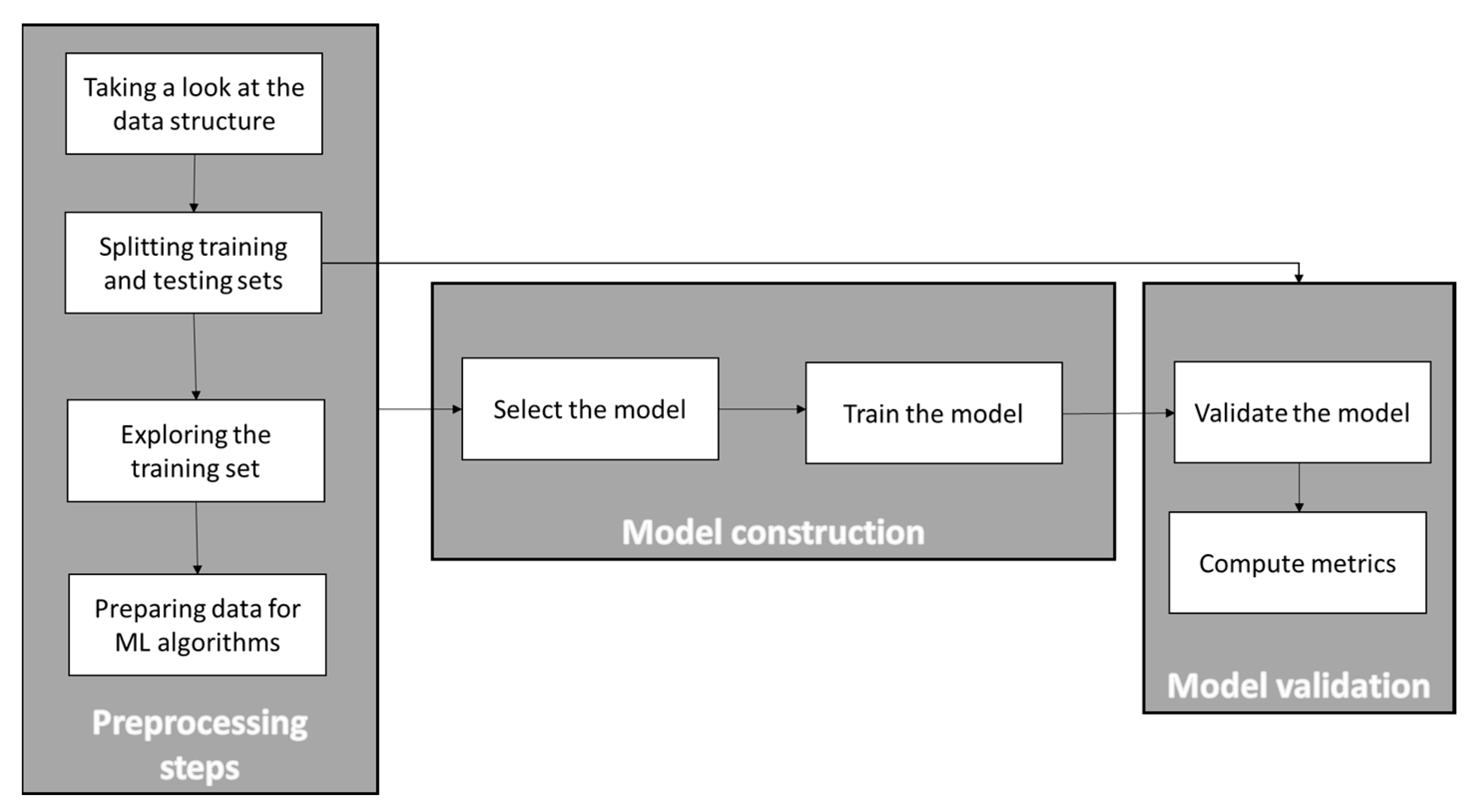
The Figure 1 shows the main steps of a typical machine learning process:

In this section, each of the steps in the figure above will be explained and applied to the selected aerodynamic databases. It is important to mention that all the research performed in this paper used Scikit-learn 0.22.1, pandas 1.0.1, matplotlib 3.1.3, and python 3.8.2 libraries, all included in the Anaconda distribution. CFD computations for the databases generation were performed with the DLR TAU code (release 2019.1.0, Spalart–Allmaras turbulence model, convergence criteria based on minimum residuals).

In order to allow other researchers to perform experiments on existing aerodynamic databases and avoid the repetition of the CFD simulations required to build such databases, Appendix A provides all the required data for free use within the research community

3.1. Data Polishing and Statistical Analysis

The first step was to quickly explore what the databases looked like. As mentioned previously, the complete databases for all the tested performed in this paper can be found in the annexes.

One of the important issues in databases for machine learning is that there are no empty values because, in case they exist, they should be substituted by the average, by zero or other values, depending on the specific case, in order to not affect the surrogate model performance. Therefore, it was checked if there were empty values for any of the variables and the result, as can be observed in the following

Table 2. Initial information of the aerodynamic databases.

NACA0012	RAE2822	DPW
Range Index: 185 entries, 0 to 184	Range Index: 122 entries, 0 to 121	Range Index: 100 entries, 0 to 99
Data columns (total 4 columns):	Data columns (total 4 columns):	Data columns (total 4 columns):
Mach: 185 non-null float64	Mach: 122 non-null float64	Mach: 100 non-null float64
AoA: 185 non-null int64	AoA: 122 non-null int64	AoA: 100 non-null int64
Cl: 185 non-null float64	Cl: 122 non-null float64	Cl: 100 non-null float64
Cd: 185 non-null float64	Cd: 122 non-null float64	Cd: 100 non-null float64
dtypes: float64 (3), int64 (1)	dtypes: float64 (3), int64 (1)	dtypes: float64 (3), int64 (1)

, was that there were no empty values in the databases.

As can be observed in the previous table, all three databases are composed of 4 columns (corresponding to the Mach, AoA, lift coefficient and drag coefficient). The data size varies depending on the configuration, the NACA0012 database has 185 rows (it means CFD computations), the RAE2822 database has 122 samples, and the DPW databases includes 100 samples.

Then, it is possible to have a look at some statistics of the aerodynamic data in the databases

Table 3. Statistics of the aerodynamic database (NACA0012).

Variable	Mach	AoA	Cl	Cd
count	185.00	185.00	185.00	185.00
mean	0.499459	9.800000	0.897379	0.144013
std	0.261579	5.978949	0.438446	0.151947
min	0.100000	0.000000	−0.000391	0.004161
25%	0.300000	5.000000	0.622582	0.020779
50%	0.500000	10.00000	0.953855	0.105718
75%	0.700000	15.00000	1.216015	0.202184
max	0.900000	20.00000	1.657733	0.692383

,

Table 4. Statistics of the aerodynamic database (RAE2822).

Variable	Mach	AoA	Cl	Cd
count	122.00	122.00	122.00	122.00
mean	0.505738	6.573770	0.788143	0.076774
std	0.265448	4.340694	0.323649	0.090517
min	0.100000	0.000000	−0.039599	0.008645
25%	0.300000	3.000000	0.553919	0.011459
50%	0.500000	6.000000	0.821918	0.024456
75%	0.700000	10.00000	0.992458	0.130592
max	0.900000	15.00000	1.434611	0.394642

and

Table 5. Statistics of the aerodynamic database (DPW).

Variable	Mach	AoA	Cl	Cd
count	100.00	100.00	100.00	100.00
mean	0.388000	6.260000	0.946160	0.058803
std	0.213333	4.296158	0.331897	0.038622
min	0.100000	0.000000	0.344904	0.009539
25%	0.200000	3.000000	0.679916	0.026364
50%	0.400000	6.000000	0.968587	0.049764
75%	0.600000	10.00000	1.198574	0.088710
max	0.800000	15.00000	1.565249	0.160681

:

In the table above, the rows labeled “count”, “mean”, “min”, and “max” correspond to the number of samples, mean value of the parameter, minimum and maximum values, respectively. The row labeled “std” shows the standard deviation of the values for this particular parameter. Rows labeled as 25%, 50%, and 75% show the percentiles, which reflect the value below which a given percentage of observations in a certain group of observations falls.

From these statistics, there is one important aspect to consider. The AoA values have a high standard deviation and this will have to be considered further when deciding how to scale the training data to not affect the model performance.

It is also possible to plot the histograms of each of the considered parameters, to better understand the type of data to deal with. The following Figure 2, Figure 3 and Figure 4 show the histograms of each variable in the database for the three cases considered:

As can be deduced from the pictures above, all the three database were generated with a Latin Hypercube Sampling (LHS) method in parameters AoA and Mach, this is why the histograms show the same bars altitude except for those cases where the CFD solver did not converge (those with highest angles of attack which did not achieve the minimum residual convergence criteria) and were eliminated from the database.

In the case of Cd, the histogram shows a strong concentration of values near to 0, and the Cl histogram shows the main concentration for values between 0.7 and 1.25, especially in the two airfoil databases.

3.2. Splitting Training and Test Sets

The next step was to split the database between train and test sets. In this example, the split was done with a pure random sampling method and considering 80% of the initial samples for the train set and the other 20% for the test set. This step could be improved by using other splitting methods (such as cross-fold validation for instances as the work performed in [21]), but since the purpose of this paper is to give a general overview of the machine learning process for aerodynamic analysis, this random sampling technique was considered.

3.3. Exploring the Training Set

Now, the kind of data that will be used to build the model is explored more in detail, as can be observed in Figure 5:

In addition, since the datasets are of a manageable size, it is also possible to compute the Pearson’s coefficient $r$ for every pair of variables, as are displayed in the following

Table 6. Pearson correlation coefficients in NACA0012 databases.

Variable	AoA	Mach	Cl	Cd
AoA	1.0	0.013024	0.788449	0.673338
Mach	0.013024	1.0	0.101251	0.57034
Cl	0.788449	0.101251	1.0	0.652496
Cd	0.673338	0.570344	0.652496	1.0

,

Table 7. Pearson correlation coefficients in RAE2822 databases.

Variable	AoA	Mach	Cl	Cd
AoA	1.0	0.018619	0.770069	0.650465
Mach	0.018619	1.0	−0.100818	0.559170
Cl	0.770069	−0.100818	1.0	0.262417
Cd	0.650465	0.559170	0.262417	1.0

and

Table 8. Pearson correlation coefficients in DPW databases.

Variable	AoA	Mach	Cl	Cd
AoA	1.0	−0.339471	0.962521	0.819541
Mach	−0.339471	1.0	−0.121352	0.080954
Cl	0.962521	−0.121352	1.0	0.892737
Cd	0.892737	0.080954	0.892737	1.0

:

In addition, one can also plot every numerical variable against any other numerical variable. In this case, since there are 4 attributes, 42 plots are obtained for each database, as can be observed in the following Figure 6, Figure 7 and Figure 8:

Since the main diagonal of these plots would be full of straight lines, instead of showing them, it is displayed as a histogram of each attribute (remember that these histograms look different with respect to the ones showed previously, since now only the training dataset is considered).

From these pictures, it can be observed that, for predicting the lift coefficient, the AoA has a very strong importance, while the Mach number is less important. However, for the prediction of the Cd, both parameters have almost the same importance, especially in the 2D cases. This aspect is less clear in the DPW test case, where the Mach number seems to be less important than the AoA for Cd prediction.

3.4. Preparing the Data for Machine Learning Algorithms

The first step here would be to handle the missing values in the database, but as it was mentioned before, the databases do not have missing values, since all the cases without solver convergence were not incorporated in the database.

Now, it is necessary to apply one of the most important transformations to the data, which is feature scaling. Machine learning algorithms do not behave well when the parameters have different ranges, and this is the case here since the scales of the AoA and the Cd for instance are very different, as it was also mentioned previously. In this research, a standard normally distributed scaling method [22] for each column in the training database (0 mean and unit variance) was used. The selected scaling method does not have a relevant impact on the results; what is really crucial is that all features are scaled in order to help machine learning methods to provide efficient predictions.

3.5. Model Construction

Until now, the problem has been stablished, the data have been obtained and examined, the training set and a test set have been sampled, and feature scaling has been performed to adapt the data for machine learning algorithms. In this subsection, a machine learning model is going to be selected and trained.

Since this paper aims to provide a global overview of the machine learning process, it is not in the scope to provide a deep evaluation of different models and tune the model parameters. Instead, only two regression models are selected and used with the default variables defined in the Scikit-learn packages:

• Linear regression [23].
• Support vector regression (gamma = “scale”, C = 1.0, epsilon = 0.1 for Cl prediction, 0.01 for Cd prediction)) [24].

3.6. Model Validation

Once the model is trained, the final step is to use it for predicting new values and validate its performance.

First, the linear regression model was tested.

Table 9. Performance metrics for the linear regression model (MAE: mean absolute error, MSE: mean squared error, R²: coefficient of determination).

Test case	NACA0012			RAE2822			DPW
Variable	MAE	MSE	R2	MAE	MSE	R2	MAE	MSE	R2
Cl	0.213361	0.064331	0.599226	0.170544	0.039926	0.725196	0.030881	0.002242	0.981537
Cd	0.048828	0.003615	0.773458	0.037094	0.002124	0.753398	0.011685	0.000197	0.853932

shows the typical regression metrics for model comparison. Figure 9 shows the comparison between true vs. predicted coefficient values with linear regression method.

Then, the support vector regression model was tested. The following

Table 10. Performance metrics for the SVR model (MAE: mean absolute error, MSE: mean squared error, R²: coefficient of determination).

Test Case	NACA0012			RAE2822			DPW
Variable	MAE	MSE	R2	MAE	MSE	R2	MAE	MSE	R2
Cl	0.087786	0.010171	0.936636	0.080280	0.008804	0.939404	0.038026	0.002941	0.975785
Cd	0.008265	0.000168	0.989469	0.009824	0.000133	0.984611	0.006637	0.000059	0.956424

shows the typical regression metrics for model comparison. Figure 10 shows the comparison between true vs. predicted coefficient values with SVR method.

As can be observed in the figures above, the SVR model behaves better than the linear regression model, as was expected. The R² metrics show reasonable accuracy values for the constructed model. Of course, a more robust cross-validation strategy, as well as the optimization of the SVR hyper parameters could have been performed, but the objective of this paper was only to give an overall view of the whole machine learning process for analysis of aerodynamic databases and prediction of aerodynamic coefficients.

4. Conclusions

This paper focuses on exploring the benefits that machine learning and data mining techniques can offer to aerodynamicists in order to extract knowledge from the CFD data and to make quick predictions of aerodynamic coefficients. The main objective of this paper has been to introduce all the steps in a typical machine learning process and apply these steps to aerodynamic databases. For this purpose, three aerodynamic databases (NACA0012 airfoil, RAE2822 airfoil and 3D DPW wing) have been used and results have demonstrated the feasibility and potential benefits of applying machine learning and data-driven techniques for aerodynamic analysis of aeronautical configurations.

As the future work, there is still further potential to be exploited: a clever generation of the samples in the initial dataset (not LHS), the use of more robust model validation strategies, such as cross-fold validation, the combination of multi-fidelity data within the aerodynamic database (e.g., CFD, wind tunnel, flight testing data, etc.), the comparison of different regression models and tuning these parameters, etc. In addition, the use of these models for uncertainty quantification is another future research topic to face.

Finally, it is important to mention that all databases used in this paper are freely available for the scientific community.

References

1. Hanna, B.N.; Dinh, N.T.; Youngblood, R.W.; Bolotnov, I.A. Machine-learning based error prediction approach for coarse-grid Computational Fluid Dynamics (CG-CFD). Prog. Nucl. Energy 2020, 118, 103140. [Google Scholar] [CrossRef]
2. Ti, Z.; Deng, X.; Yang, H. Wake modeling of wind turbines using machine learning. Appl. Energy 2020, 257, 114025. [Google Scholar] [CrossRef]
3. Zhao, Y.; Akolekar, H.D.; Weatheritt, J.; Michelassi, V.; Sandberg, R.D. RANS turbulence model development using CFD-driven machine learning. J. Comput. Phys. 2020, 411, 109413. [Google Scholar] [CrossRef] [Green Version]
4. Zhu, L.; Zhang, W.; Kou, J.; Liu, Y. Machine learning methods for turbulence modeling in subsonic flows around airfoils. Phys. Fluids 2019, 31, 015105. [Google Scholar] [CrossRef]
5. Holland, J.R.; Baeder, J.D.; Duraisamy, K. Towards integrated field inversion and machine learning with embedded neural networks for rans modeling. In Proceedings of the AIAA Scitech 2019 Forum, San Diego, CA, USA, 7–11 January 2019. [Google Scholar]
6. Paulete-Periáñez, C.; Esther, A.-P.; Carlos, L. Surrogate modelling for aerodynamic coefficients prediction in aeronautical configurations. In Proceedings of the 8th European Conference for Aeronautics and Space Sciences (EUCASS), Madrid, Spain, 1–4 July 2019. [Google Scholar] [CrossRef]
7. Venturi, S.; Sharma Priyadarshini, M.; Panesi, M. A Machine Learning Framework for the Quantification of the Uncertainties Associated with Ab-Initio Based Modeling of Non-Equilibrium Flows. In Proceedings of the AIAA Scitech 2019 Forum, San Diego, CA, USA, 7–11 January 2019. [Google Scholar]
8. Buisson, B.; Lakehal, D. Towards an integrated machine-learning framework for model evaluation and uncertainty quantification. Nucl. Eng. Des. 2019, 354, 110197. [Google Scholar] [CrossRef]
9. Yan, X.; Zhu, J.; Kuang, M.; Wang, X. Aerodynamic shape optimization using a novel optimizer based on machine learning techniques. Aerosp. Sci. Technol. 2019, 86, 826–835. [Google Scholar] [CrossRef]
10. Wu, J.; Xiao, H.; Paterson, E. Physics-informed machine learning approach for augmenting turbulence models: A comprehensive framework. Phys. Rev. Fluids 2018, 3, 074602. [Google Scholar] [CrossRef] [Green Version]
11. Dupuis, R.; Jean-Christophe, J.; Pierre, S. Aerodynamic Data Predictions for Transonic Flows via a Machine-Learning-based Surrogate Model. In Proceedings of the 2018 AIAA/ASCE/AHS/ASC Structures, Structural Dynamics, and Materials Conference, Orlando, FL, USA, 8–12 January 2018. [Google Scholar]
12. Zhang, Y.; Woong, J.S.; Dimitri, N.M. Application of convolutional neural network to predict airfoil lift coefficient. In Proceedings of the 2018 AIAA/ASCE/AHS/ASC Structures, Structural Dynamics, and Materials Conference, Orlando, FL, USA, 8–12 January 2018. [Google Scholar]
13. Yan, C. Wind Turbine Wakes: From Numerical Modeling to Machine Learning. Ph.D. Thesis, University of Delaware, Newark, DE, USA, 2018. [Google Scholar]
14. Secco, N.R.; De Mattos, B.S. Artificial neural networks to predict aerodynamic coefficients of transport airplanes. Aircr. Eng. Aerosp. Technol. 2017, 89, 211–230. [Google Scholar] [CrossRef]
15. Kou, J.; Zhang, W. Multi-kernel neural networks for nonlinear unsteady aerodynamic reduced-order modeling. Aerosp. Sci. Technol. 2017, 67, 309–326. [Google Scholar] [CrossRef]
16. Morshedizadeh, M. Condition Monitoring of Wind Turbines Using Intelligent Machine Learning Techniques. Ph.D. Thesis, University of Windsor, Windsor, ON, Canada, 2017. [Google Scholar]
17. Andrés-Pérez, E.; Carro-Calvo, L.; Salcedo-Sanz, S.; Martin-Burgos, M.J. Aerodynamic Shape Design by Evolutionary Optimization and Support Vector Machines. In Application of Surrogate-based Global Optimization to Aerodynamic Design; Springer: Cham, Switzerland, 2016; pp. 1–24. [Google Scholar]
18. Viúdez-Moreiras, D.; Andrés-Pérez, E.; González-Juárez, D.; Burgos, M.J.M. Performance Comparison of Kriging and Svr Surrogate Models Applied to the Objective Function Prediction within Aerodynamic Shape Optimization. In Proceedings of the VII European Congress on Computational Methods in Applied Sciences and Engineering (ECCOMAS Congress 2016), Crete, Greece, 5–10 June 2016. [Google Scholar] [CrossRef] [Green Version]
19. Wang, Q.; Qian, W.; He, K. Unsteady aerodynamic modeling at high angles of attack using support vector machines. Chin. J. Aeronaut. 2015, 28, 659–668. [Google Scholar] [CrossRef] [Green Version]
20. Fossati, M. Evaluation of Aerodynamic Loads via Reduced-Order Methodology. AIAA J. 2015, 53, 2389–2405. [Google Scholar] [CrossRef]
21. Chen, S.; Chen, K.; Xu, C.; Lan, L. Flexible ranking extreme learning machine based on matrix-centering transformation. In Proceedings of the 2018 International Joint Conference on Neural Networks (IJCNN); Institute of Electrical and Electronics Engineers (IEEE): New York, NY, USA, 2018; pp. 1–8. [Google Scholar]
22. Yao, J.; Moawad, A. Vehicle energy consumption estimation using large scale simulations and machine learning methods. Transp. Res. Part C: Emerg. Technol. 2019, 101, 276–296. [Google Scholar] [CrossRef]
23. Dube, P.; Hiravennavar, S. Machine Learning Approach to Predict Aerodynamic Performance of Underhood and Underbody Drag Enablers SAE Technical Paper 2020-01-0684; SAE Technical Paper: Warrendale, PA, USA, 2020. [Google Scholar] [CrossRef]
24. Download CitationChen, S.; Gao, Z.; Zhu, X.; Du, Y.; Pang, C. Unstable unsteady aerodynamic modeling based on least squares support vector machines with general excitation. Chin. J. Aeronaut. 2020. [Google Scholar] [CrossRef]
Figure 1. Main steps of a machine learning process (preprocessing–model construction–model validation).
Energies 13 05807 g001
Figure 2. Histograms of the variables in the NACA0012 database (X-axis shows the value of the parameter while Y-axis shows the number of occurrences of that value in the database).
Energies 13 05807 g002
Figure 3. Histograms of the variables in the RAE2822 database (X-axis shows the value of the parameter while Y-axis shows the number of occurrences of that value in the database).
Energies 13 05807 g003
Figure 4. Histograms of the variables in the DPW database (X-axis shows the value of the parameter while Y-axis shows the number of occurrences of that value in the database).
Energies 13 05807 g004
Figure 5. Training set in the NACA0012 (a), RAE2822 (b) and DPW (c) databases (left: Mach versus AoA distribution of the database samples, middle: lift coefficient curves of the database samples, right: drag coefficient curves of the database samples).
Energies 13 05807 g005
Figure 6. Exploring training set in the NACA0012 database (correlation matrix plot).
Energies 13 05807 g006
Figure 7. Exploring training set in the RAE2822 database (correlation matrix plot).
Energies 13 05807 g007
Figure 8. Exploring training set in the DPW database (correlation matrix plot).
Energies 13 05807 g008
Figure 9. True vs. predicted coefficient values with linear regression method: NACA0012 (a) RAE2822 (b) and DPW (c) databases (left: lift coefficient, right: drag coefficient).
Energies 13 05807 g009
Figure 10. True vs. predicted coefficient values with SVR method: NACA0012 (a) RAE2822 (b) and DPW (c) databases (left: lift coefficient, right: drag coefficient).
Energies 13 05807 g010