Abstract
The distribution side of the traditional power grid is changing as the users (known as prosumers) can inject power to the grid. However, uncontrollable injection of power can destabilize the grid. Thus, the stability of the grid must be maintained. Since the prosumers are self-interested entities, they will take their actions to maximize their own pay-offs. We formulate the problem as a non-cooperative game theoretic problem where the magnitude of the voltage must be within an acceptable limit at each node of the power network. Since the power-flow equations must be satisfied at each node, it becomes a coupled constrained game where the constraints are the same across the prosumers. We propose a distributed penalty based algorithm which converges to an equilibrium. In this mechanism, the prosumers are quoted a price based on the active and reactive power drawn or injected to the power grid. The algorithm is easy to implement and it converges to an efficient solution which maximizes the sum of the utilities of the prosumers while maintaining the grid’s stability.
1. Introduction
The proliferation of the distributed energy resources (e.g., Photo voltaic (PV) arrays, solar rooftops, energy storage units) have transformed the notion of traditional consumers of energy. The consumers can now also produce and supply power to the grid. We denote the consumers with the capability of producing energies as prosumers. The users are also using electric vehicles (EVs) which require energy for charging, but can also provide energy back to the grid by discharging. However, as the distribution network is going through rapid transformation it may create instabilities into the grid. It is worthwhile to remember that a centralized solution is not implementable in a system of thousands of household entities and their controllable devices since the homeowners or prosumers take their decision which will benefit them. Thus, each prosumer takes its own decision which will maximize its own objective without coordinating with other prosumers. Thus, the question is how to control different self-interested entities while maintaining the stability of the grid?
In order to answer the above question, we consider a system where prosumers can sell and buy energies from the grid. For each time period, each prosumer decides how much to buy and how much to sell depending on its own utility function, selling and buying price. The power drawn from or injected into the grid must follow the Kirchoff’s current and voltage laws. We consider a radial distribution network where each node consists of a subset of prosumers. At each node, the magnitude of the voltage must be maintained within an acceptable range to maintain stability of the grid. The voltage magnitude is obtained by solving a set of non-linear active and reactive power flow equations which are very difficult to solve. Note that the active and reactive powers injected or drawn are decided by the prosumers. Thus, each prosumer needs to decide how much to buy or sell while maintaining the stability of the grid.
Since the non-linear AC power flow equations are non-convex, we consider a linearized power flow equations which are reasonable and considered in the literature [1,2]. However, each prosumer only solves its own optimization problem, hence, we consider a game theoretic setting to characterize the strategic interactions among multiple prosumers. The prosumers have the same constraint that the voltage magnitude must be within an acceptable range at each node. Hence, this leads to a coupled constrained game [3]. We seek to obtain a generalized Nash equilibrium (GNE) which is the relevant equilibrium concept for a coupled constrained game. The coupled constrained game is difficult to solve as the strategy space depends on the strategies of the other players and the power system parameters such as line impedances. However, a prosumer is unaware of the power network (the reactance, resistance, and the number of nodes) and is also unaware of the decisions of other prosumers.
We propose a distributed algorithm to obtain a GNE. GNE is not unique in general, however, the GNE obtained using the distributed algorithm is an efficient solution i.e., it maximizes the sum of the utilities of the prosumers. In the distributed algorithm, a controller which has knowledge of the power network and its parameters quotes a penalty price to the prosumers if the voltage magnitude constraint is not satisfied at a node. For example, if the voltage magnitude is lower than a specified value, then, the prosumers are penalized for selling energies and vice versa. Note that prosumers may also sell reactive power since the distributed energy resources are converted to the AC power using inverter. Excessive reactive power is also penalized if the voltage magnitude becomes small because supply exceeds the demand.
When the voltage magnitude exceeds the upper limit, the penalty for drawing power is increased till the voltage magnitude remains within an acceptable limit. We show that such an iterative price algorithm converges to a GNE. The convergence is also very fast and thus, can readily be implemented in practice. Numerically, we show that the utility of our algorithm in maintaining the stability of the grid. The penalty parameters depends on the number of links a node has and the impedance values between those links since power needs to be rerouted to the neighboring nodes if the supply and demand does not match at a given node.
We summarize our contributions in the following:
- We mathematically model strategic prosumers who take their decisions in order to maximize their own objectives without coordinating with other prosumers while maintaining the voltage stability in the grid using a game theoretic setting.
- We propose a practically implementable algorithm which converges to the efficient GNE.
- We show that there exists a distributed algorithm where a controller at each node selects penalty prices for violating a constraint.
The rest of the paper is organized as the following: Section 2 compares our work with the existing literature. Section 3 describes the system parameters, and the objective each prosumer tries to optimize. In Section 4 we propose a distributed algorithm which converges to a GNE. Section 5 empirically demonstrates the strength of our algorithm in mitigating the voltage constraint violation. We conclude and provide future research direction in Section 6.
2. Related Literature
Demand response pricing has already been studied [4,5,6,7,8,9]. Real time pricing has also been considered [10,11,12,13,14,15,16]. However, these papers did not consider that the users can also sell energies back to the grid. Naturally, they did not consider the AC power flow equations while coming up with the prices. Energy exchange among the users in a micro-grid setting has been considered [3,17,18,19,20]. Though these papers considered that the users can sell back energies, they did not consider non-linear AC power flow equations and the power network structure.
Recent papers [1,2,21,22,23] have considered the control of power of prosumers in order to maintain the voltage stability. These papers assumed a centralized optimization problem with a distributed algorithm for maintaining the stability. However, in a smart grid, each prosumer takes its own decision. Hence, it is difficult to control each prosumer. Thus, game theoretic notion is better adapted to study the strategic interaction among prosumers. In a game theoretic setting, it is not apriori clear whether an equilibrium exists and whether an equilibrium can be implemented in practice (if exists). Articles [24,25,26] considered a game theoretic setting to study the interaction among multiple prosumers. However, these papers did not consider any distributed algorithm which can implement the equilibrium strategy. We provide a distributed algorithm which can be implemented in practice. The distributed algorithm converges to a generalized NE, and we show that the GNE is efficient.
The article [27] considered a distributed energy management system for a cooperative multi-agent system. In contrast, we consider a non co-operative game where each prosumer takes its own decision without coordinating others. We also considered the stability of the grid unlike in [27]. The papers [28,29] proposed a distributed algorithm for controlling agents. However, in the game theoretic setting each agent takes its own decision. Further, the stability constraint where the voltage magnitude must be within the acceptable limit has not been considered in the above papers. [30,31] consider incentive mechanisms for promoting sharing of energies among different consumers. However, the stability of the grid is not considered. Further, we formulate the problem as a game theoretic setting and propose distributed algorithm which converges to an equilibrium strategy.
3. System Model and Problem Formulation
In this section, we first, describe the prosumers and their decision variables in Section 3.1. Subsequently, we describe the power flow equations as the prosoumers inject/draw power from the grid in Section 3.2. In Section 3.3, we describe the utilities of the prosumers. Finally, in Section 3.4 we describe the optimization problem that each prosumer tries to solve.
3.1. Prosumer’s Decision
Each prosumer j decides the power it will buy during time period . The duration is chosen depending on how fast the prosumers can update their decisions. Most often in the real time setting varies between 5 min to 15-min. However, can be easily adapted to a much granular level. Note that the prosumer can also sell amount of power during time period . A prosumer can sell its power by discharging from its battery or from the renewable energy resources. Note that a prosumer also represents one who does not have any distributed resources or storage unit.
Some users may have a deferrable load. The demand for those load only need to be fulfilled within a certain deadline. For example, the EV needs to be ready before 8 am (e.g., if the user is going to work). However, the individual load may vary over time. We denote the set of deferrable appliances as . Suppose the load assigned to appliance j of user i is for the time duration . Hence, we have
where is the amount of energy required for appliance j before its deadline .
The power demand of prosumer i during time , must satisfy the following–
where , and are known beforehand.
Each prosumer has a renewable energy harvesting device which harvests amount of power (A prosumer may not have any renewable energy harvesting device. In that case, the renewable energy will be 0.) during time . The prosumer i may also have a battery with capacity . If the prosumer does not have any battery then is 0. The state of the battery is . The amount of energy discharged from the battery is , and charged to the battery is . Thus, we have
Note that the renewable energy generation is a random process. Hence, a prosumer will only have the estimate of , rather than the exact realized value. Note that we assume that during the time interval is constant. If is small, it is a reasonable assumption.
The state of the battery can not be less than 0. The state of the battery is also required to be a specific value at the end of the horizon. Most often, the state of the battery is kept to be same as the start of the day. Thus, we have
Thus, the total power consumption of prosumer i during time is given by
where and are respectively the discharging, and charging efficiency from the battery. Note that only a portion of energy bought by the prosumer can be used because of the transmission loss.
3.2. Power Flow Constraint
When a prosumer injects or draws power, the power flow equations must be satisfied at every time instance. We also characterize the active and reactive power flow equations as DC power is converted to AC power when battery is discharged.
3.2.1. Inverter
The distributed energy resources are converted in AC power via an inverter. The reactive power provided by the inverter is and the power capacity of the inverter is . Hence, we must have
Recall that is the real power discharged from the Battery or distributed energy resources (if there is no battery).
3.2.2. Power Flow Equations
We, now, describe the power flow equations which must be satisfied. The power flow network consists of nodes and edges . An edge or link exists between two nodes if the two nodes are connected.
Let us assume that the set of prosumers belong to the node i in the power network. Note that in general, the cardinality of the set can be 1 which denotes that each prosumer’s end can be treated as a node. The root of the tree is the feeder with a fixed voltage and power injection, and is denoted by bus 0. We denote the other buses as . For each link , let be the complex impedance. Let be the complex current flowing during time and be the real and passive power respectively flowing through edge during time .
Let and be the total real load and passive load of all the prosumers at node j. Then,
We are now ready to represent the power flow model. For all links we must have
where . The equality constraints in the system of equations in (8) describe the physical power flow models. Because of the non-linearity, the values of the voltage may not be uniquely determined even when the power load , are specified. There can be no solution or multiple solutions.
The following voltage constraint must be satisfied at each node
where and correspond to the maximum and minimum voltage limit respectively at node i.
Though the constraints specified in system of equations in (8) are non-linear, we consider a linearized version (i.e. ) specified by the following equation
where , , , and
where is the set of edges in the path between Bus 0 and Bus i. Linearized model is a good representation of the radial distribution network. It also has another advantage– unlike the non-linear model, for a given p and q the voltage equations can be solved accurately. Though we do not consider any limit on the power flow explicitly, the constraint on the magnitude of the voltage implicitly limits the amount of active and reactive power flow. We can add constraints on the power magnitude without losing the complexity of the problem. For example, constraint such as is linear and convex. Thus, the problem will remain convex and our proposed algorithm can be adapted to handle the above constraint.
3.3. Prosumer’s Utility
Each prosumer i attains an utility depending on the amount of power consumed. The utility of the user depends on the the consumption . The utility of a prosumer/user is the economic value obtained by consuming or availing a service. If a prosumer/user consumes more energy, the utility will increase. The utility of a prosumer inherently depends on its willingness to consume. For example, if a prosumer consumes significantly less amount of energy compared to its desired value, its utility will be smaller. Similarly, if a prosumer wants to set its temperature at a certain value, the utility will be smaller if it is set at a value different from its preferred value.
The prosumer also has to pay amount for buying energy as the price charged by the utility company is in $/kwh. Note that a prosumer is charged depending on the energy consumption, not on the power consumption. Similarly, the prosumer also gets amount for selling energy. We assume that to avoid trivial solutions.
Note that the utility can have time correlated component which can easily be incorporated in the model. Those utility functions can be represented as . On the other hand the utility may be separable across the time. Without loss of generality, we consider that the utility function is given by .
Assumption 1.
We assume that is increasing and concave function.
The concavity assumption stems from the fact that if a prosumer consumes more energy the rate of change of valuation decreases.
3.4. Optimization Problem of Prosumer
Each prosumer is a selfish entity which only wants to optimize its own payoff. Thus, each prosumer solves the following problem
Note that it is a coupled constrained game since the constraint in (10) is common to all the prosumers.
3.5. Strategic Interactions
Each prosumer tries to solve its own optimization problem in (12). Thus, we consider a non co-operative game theoretic setting where each prosumer takes its own decision. The constraint in (10) is the same across the prosumers. Thus, the feasible strategy space of a prosumer inherently depends on the actions of others. However, the game is a coupled-constrained game since the constraints are common to the prosumers. We, thus, seek to obtain a generalized Nash equilibrium.
Before defining the generalized Nash equilibrium formally, we introduce some notations. We denote the objective function of each prosumer i as . We also represent the decision variable of prosumer i as . Suppose is a strategy profile where is the set of feasible strategies.
Definition 1.
The strategy profile is a generalized Nash equilibrium if , .
Thus in a generalized Nash equilibrium a prosumer can not find another feasible strategy which can give a better utility if the strategies of the other prosumers remain fixed.
4. Algorithm
In this section, we describe the algorithm DIST-OPT which converges to the generalized Nash equilibrium.
We propose a distributed algorithm which converges to the generalized Nash equilibrium.
- Initialize , , for .
- Each prosumer solves the following problem
- Prosumers inform their latest strategy at k-th iteration. If , the algorithm terminates. Otherwise, it proceeds in the following.
- Controller at bus i measures the voltage at node i.
- Controller at bus i updates , and according to the followingwhere is the step parameter.
A controller is located at each node, it knows the local information such as the neighboring nodes, the resistance and reactance values between its neighbors. These is the only information required for the controller to implement the algorithm DIST-OPT. We assume that a controller at the bus will communicate with the prosumers.
Note that a prosumer i pays a penalty if it injects too much active power and reactive power respectively. On the other hand, if it draws too much active power it also pays the penalty . One key difference with the traditional price is that such a price is charged based on the power. It is not based on the energy unlike the real time prices for the energy consumption.
Note that the penalty parameter is not the same for all the prosumers, rather it depends on the node set it belongs. It also depends on the impedances between the neighboring links. Since prosumers always inject reactive power, thus, reactive power is not penalized when the voltage magnitude is higher than the threshold. However, when the voltage magnitude is smaller than the acceptable value, reactive power is also penalized.
The following theorem entails that even though each prosumer takes its own decision, it converges to the generalized Nash equilibrium.
Theorem 1.
The algorithm DIST-OPT converges to a generalized Nash equilibrium.
Outline of Proof: The algorithm DIST-OPT is a primal-dual gradient algorithm. The penalty prices correspond to the dual variables. Thus, the proof follows from the theory of convex optimization [32].
Since the optimization problem at each prosumer’s end is a convex optimization problem, thus, the algorithm can be implemented in practice even when there are large number of nodes.
Note that there can be multiple generalized NE. For example, suppose that there are two prosumers and one node, the cost of energy is zero, and the minimum amount of energy requirement for each of the prosumers is zero. Now, one of the prosumers can draw a lot of power till the point the voltage magnitude becomes equal to the maximum limit. The other prosumer can not draw any power as it will make the voltage exceeds the maximum limit. Thus, there can be multiple equilibria. We, thus, want a generalized NE which is close to an efficient solution (if any), i.e., the strategy is closer to the optimal solution of the problem where sum of the prosumers’ objectives are maximized subject to the set of constraints. The generalized NE obtained from the Algorithm DIST-OPT is indeed an efficient solution which is formally stated in the following.
Theorem 2.
Suppose the Algorithm DIST-OPT converges to a generalized NE then the above strategy is also a solution of the following problem
Proof: Note that the optimization problem in (15) is exactly equal to the optimization problem in (12). Since GNE obtained using the algorithm DIST-OPT is an optimal solution of (12), thus, it is also an optimal solution of (15).
Thus, the generalized NE attained also maximizes the sum of the utilities of the prosumers. Hence, the generalized NE attained by the algorithm DIST-OPT is efficient.
Execution Time: Note that DIST-OPT algorithm gives an optimal solution of a strictly convex optimization problem. DIST-OPT is a primal dual gradient algorithm. Thus, the convergence is fast and polynomial in and polynomial in the dimension of the decision variables. Thus, even when the number of nodes increases, the run time only scales in a polynomial order. In our simulations, we also show that the convergence is fast.
5. Numerical Results
In this section, we demonstrate our proposed architecture on a simulated power grid system. We, first, describe our set-up. Subsequently, we describe the insights we obtain from the simulated system.
5.1. Simulation Set-Up
We run the proposed algorithm in 5-min interval for 24 h. So, there are 288-time intervals. We assume that the renewable energy is harvested according to a truncated Gaussian distribution with mean 5 kwh and variance 2 kwh. The storage unit is assumed to be of capacity uniformly distributed in the interval kwh across the users. Initial battery level is assumed to be 0 i.e., it is fully discharged. The prices for the conventional energy is assumed to be governed by Time-of-Use (ToU) time scale. Thus, the cost of buying energy varies over time. Currently, the selling price to the grid is assumed to be the same as the buying price in the net-metering scheme. However, when the renewable energy will have higher penetration net metering scheme is not profitable to the retailers. Thus, we consider that the selling price at time t, is a random variable uniformly distributed between where is the real-time buying price.
Similar to [33], the user’s utility for energy x is taken to be of the form . The parameter is the maximum demand of the users. We vary over time for each user. Specifically, during peak time (time between 9 am to 6 pm) we consider is uniformly distributed between kwh. On the other hand, during the off-peak hours, we consider it as uniformly distributed in the interval -kwh. The acceptable voltage range is assumed to be between volt p.u. The resistance and reactance of the edges are assumed to be -ohm/km. We also consider a 14-node distribution system with radial network. The distribution network setup is exactly equal to one considered in [1], we have also shown in Figure 1. The number of prosumers are considered to be 1000 which are uniformly distributed over the network.
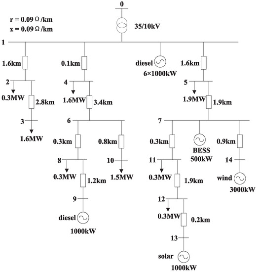
Figure 1.
The distribution network configuration we consider [1] for a certain realization of load and supply.
Note that each prosumer solves its own optimization problem which we have solved using CVX toolbox of MATLAB. The algorithm converges very fast with mostly within 20–25 iterations. The algorithm converges within 3.2 s on an average where the average is taken over 25 runs. We consider as .
5.2. Results
5.2.1. Voltage Variation
We have compared our algorithm (Figure 2 compared to the one where there is no control mechanism. It shows how our algorithm DIST-OPT maintains the voltage magnitude compared to the setting where there is no control mechanism. As it is evident from the Figure 2 and Figure 3 that our algorithm maintains the voltage stability compared to the setting where there is no control mechanism. Note that during the peak time (off-peak, respv.) the voltage tends to exceed (go below, respv.) the upper (lower, respv.) limit without the control mechanism.
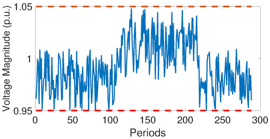
Figure 2.
The blue line shows the variation of the magnitude of voltage when we implement our algorithm. The red lines show the acceptable limits.
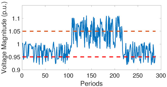
Figure 3.
The blue line shows the variation of the magnitude of voltage where there is no control mechanism. The red lines show the acceptable limits.
5.2.2. Penalty Prices
Figure 4 shows the variation of the total penalty prices to implement DIST-OPT algorithm at a node. Note that during the peak period, the penalty is imposed for drawing power. On the other hand during the off-peak period, the penalty is imposed for injecting power. Hence, it shows that we need to implement penalties both for drawing and injecting power. The prices are the highest at nodes 3 and 12 since the resistances are higher between those nodes and neighbours.
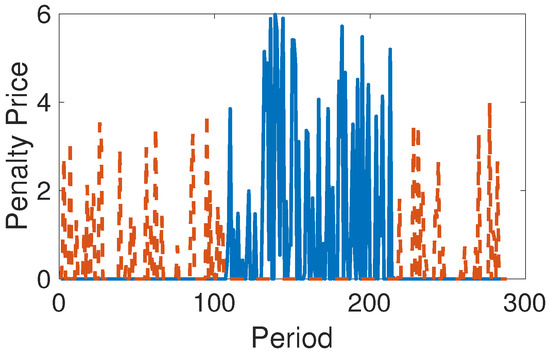
Figure 4.
The solid line shows the total penalty price ($ per MW) for drawing power and the broken line shows the total penalty price ($ per MW) for injecting power.
5.2.3. Impact of Storage Units
Figure 5 shows the impact of an increase in the household storage unit on the prices. Note that the average price for injecting power as well as the price for drawing power decreases. Intuitively, as the capacity increases, prosumers can optimize more efficiently, thus, the average penalty reduces.
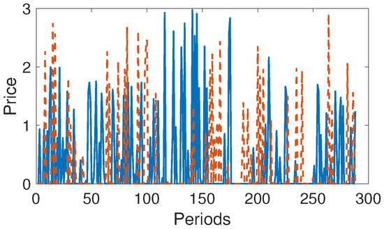
Figure 5.
The solid line shows the penalty price ($ per MW) for drawing power and the broken line shows the penalty price ($ per MW) for injecting power. The storage unit of household is now uniformly distributed between [0,10] kwh.
Though the average penalty price reduces overall, prices at individual time period may increase. Note that the price for power drawn during the off-peak increases since prosumers now want to store more energies during the off-peak periods. Similarly, the prosumers can also supply excess energies to the other prosumers during the peak period. Thus, the prices for injecting power increases during the peak time. It also shows that if the storage has a higher penetration level, the prices need to be computed carefully.
5.2.4. Penalty Price for Reactive Power Injection
Figure 6 depicts the total penalty prices for the reactive power injected into the network. It shows that the prices are positive mostly during the off-peak time. Intuitively, during the off-peak period the demand is lower, thus, the voltage magnitude is small. Thus, if prosumers inject power, it is penalized in order to maintain the voltage magnitude above the acceptable limit. On the other hand, during the peak period the demand is large, thus, the penalty price for injecting power decreases in order to incentivize the prosumers to inject more power. The prices are higher at nodes 3 and 12 since the reactances are higher.
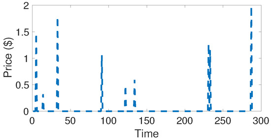
Figure 6.
The total penalties ($ per MW) for reactive power across the network at different times.
5.2.5. Energy Injected from the Prosumers
Figure 7 depicts the total amount of energies injected from the prosumers to the grid. Note that the prosumers inject a larger amount of energy to the grid during the peak period. Intuitively, the prices are higher during the peak period, thus, the prosumers tend to inject a larger amount of energy during the peak period in order achieve a larger profit. Figure 7 also shows that when the storage capacities of the prosumers are larger, more energy is injected into the grid during the peak period. This is because prosumers can also store energy during the off-peak period and give back energy during the peak period. Hence, the energy given back during the off-peak period decreases and the energy given back during the peak period increases.
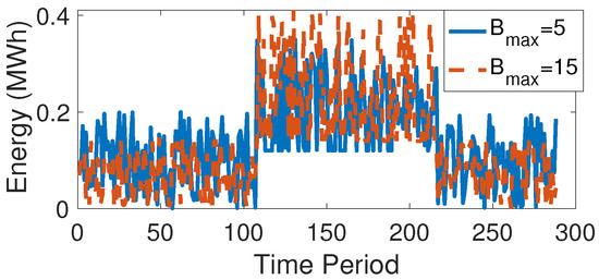
Figure 7.
The total amount of Energy given back to the Utility as a function of time. The solid line represents the total amount of energy given back when kWh and the broken line represents the total amount of energy given back when kWh. Recall that each prosumer’s capacity is uniformly distributed between .
6. Conclusions and Future Work
We consider a scenario where the prosumers inject or draw power from the grid. The solution of power flow equations may violate the acceptable voltage magnitudes at various nodes of the power system if the prosumers draw or inject too much power. Thus, we consider a distributed control mechanism to maintain the voltage stabilities. However, the voltage stability constraint depends on the decisions of all the prosumers. Each prosumer takes its own decision without coordinating with others. Thus, developing an optimal distributed control mechanism is inherently challenging. We formulate the problem as a coupled constrained game where each prosumer maximizes its own payoff subject to the common constraint of non-linear power flow equations. We seek to obtain a generalized Nash equilibrium,. We linearize the power flow equations and propose a distributed iterative algorithm which converges to a generalized Nash equilibrium. It induces a penalty price (negative or positive) based on the power if the power flow equations violate the voltage magnitude. Our proposed algorithm converges to an efficient solution i.e. it is an optimal solution of the joint optimization problem of maximizing the sum of the objectives of the prosumers. Our numerical analysis shows that such a mechanism can maintain the stability of the grid and can be implemented in practice.
Our work can be extended in several directions. The characterization of algorithm for AC power flow model is left for the future. We expect that the tools which we have developed will provide the basis for the AC power flow model. The uncertainties of the renewable energies have not been considered as we consider a real-time market. However, the energy market operates in day-ahead setting as well as real-time setting. Hence, the characterization of an equilibrium in a day-ahead setting is also left for the future.
Author Contributions
A.G. is responsible for Conceptualization, Methodology, Simulation, Formal Analysis, and Writing–original Draft preparation; V.A. is responsible for Conceptualization, Writing, and Editing Draft. All authors have read and agree to the published version of the manuscript.
Funding
This research was funded in part by US National Science Foundation under Grant CCF-1527486.
Conflicts of Interest
The authors declare no conflict of interest.
References
- Shi, W.; Li, N.; Chu, C.; Gadh, R. Real-Time Energy Management in Microgrids. IEEE Trans. Smart Grid 2017, 8, 228–238. [Google Scholar] [CrossRef]
- AlSkaif, T.; van Leeuwen, G. Decentralized Optimal Power Flow in Distribution Networks Using Blockchain. In Proceedings of the 2019 International Conference on Smart Energy Systems and Technologies (SEST), Porto, Portugal, 9–11 September 2019; pp. 1–6. [Google Scholar] [CrossRef]
- Ghosh, A.; Aggarwal, V.; Wan, H. Strategic Prosumers: How to Set the Prices in a Tiered Market? IEEE Trans. Ind. Inform. 2019, 15, 4469–4480. [Google Scholar] [CrossRef]
- Albadi, M.H.; El-Saadany, E.F. Demand Response in Electricity Markets: An Overview. In Proceedings of the 2007 IEEE Power Engineering Society General Meeting, Tampa, FL, USA, 24–28 June 2007; pp. 1–5. [Google Scholar] [CrossRef]
- Li, N.; Chen, L.; Low, S.H. Optimal demand response based on utility maximization in power networks. In Proceedings of the 2011 IEEE Power and Energy Society General Meeting, Detroit, MI, USA, 24–28 July 2011; pp. 1–8. [Google Scholar] [CrossRef]
- Rahimi, F.; Ipakchi, A. Demand Response as a Market Resource Under the Smart Grid Paradigm. IEEE Trans. Smart Grid 2010, 1, 82–88. [Google Scholar] [CrossRef]
- Jiang, L.; Low, S. Real-time demand response with uncertain renewable energy in smart grid. In Proceedings of the 2011 49th Annual Allerton Conference on Communication, Control, and Computing (Allerton), Monticello, IL, USA, 28–30 September 2011; pp. 1334–1341. [Google Scholar] [CrossRef]
- Aalami, H.; Yousefi, G.R.; Moghadam, M.P. Demand Response model considering EDRP and TOU programs. In Proceedings of the 2008 IEEE/PES Transmission and Distribution Conference and Exposition, Chicago, IL, USA, 21–24 April 2008; pp. 1–6. [Google Scholar] [CrossRef]
- Nguyen, H.K.; Song, J.B.; Han, Z. Demand side management to reduce Peak-to-Average Ratio using game theory in smart grid. In Proceedings of the 2012 Proceedings IEEE INFOCOM Workshops, Orlando, FL, USA, 25–30 March 2012; pp. 91–96. [Google Scholar] [CrossRef]
- Chen, Z.; Wu, L.; Fu, Y. Real-Time Price-Based Demand Response Management for Residential Appliances via Stochastic Optimization and Robust Optimization. IEEE Trans. Smart Grid 2012, 3, 1822–1831. [Google Scholar] [CrossRef]
- Yoon, J.H.; Baldick, R.; Novoselac, A. Dynamic Demand Response Controller Based on Real-Time Retail Price for Residential Buildings. IEEE Trans. Smart Grid 2014, 5, 121–129. [Google Scholar] [CrossRef]
- Maharjan, S.; Zhu, Q.; Zhang, Y.; Gjessing, S.; Basar, T. Dependable Demand Response Management in the Smart Grid: A Stackelberg Game Approach. IEEE Trans. Smart Grid 2013, 4, 120–132. [Google Scholar] [CrossRef]
- Yu, M.; Hong, S.H. A Real-Time Demand-Response Algorithm for Smart Grids: A Stackelberg Game Approach. IEEE Trans. Smart Grid 2016, 7, 879–888. [Google Scholar] [CrossRef]
- Conejo, A.J.; Arroyo, J.M.; Alguacil, N.; Guijarro, A.L. Transmission loss allocation: A comparison of different practical algorithms. IEEE Trans. Power Syst. 2002, 17, 571–576. [Google Scholar] [CrossRef]
- Eksin, C.; Delic, H.; Ribeiro, A. Demand Response Management in Smart Grids With Heterogeneous Consumer Preferences. IEEE Trans. Smart Grid 2015, 6, 3082–3094. [Google Scholar] [CrossRef]
- Ghosh, A.; Aggarwal, V. Control of Charging of Electric Vehicles though Menu-based Pricing. IEEE Trans. Smart Grid 2018, 9, 5918–5929. [Google Scholar] [CrossRef]
- Lee, J.; Guo, J.; Choi, J.K.; Zukerman, M. Distributed Energy Trading in Microgrids: A Game-Theoretic Model and Its Equilibrium Analysis. IEEE Trans. Ind. Electron. 2015, 62, 3524–3533. [Google Scholar] [CrossRef]
- Saad, W.; Han, Z.; Poor, H.V. Coalitional Game Theory for Cooperative Micro-Grid Distribution Networks. In Proceedings of the 2011 IEEE International Conference on Communications Workshops (ICC), Kyoto, Japan, 5–9 June 2011; pp. 1–5. [Google Scholar] [CrossRef]
- Wu, C.; Mohsenian-Rad, H.; Huang, J.; Wang, A.Y. Demand side management for Wind Power Integration in microgrid using dynamic potential game theory. In Proceedings of the 2011 IEEE GLOBECOM Workshops (GC Wkshps), Houston, TX, USA, 5–9 December 2011; pp. 1199–1204. [Google Scholar] [CrossRef]
- Saad, W.; Han, Z.; Poor, H.V.; Başar, T. A noncooperative game for double auction-based energy trading between PHEVs and distribution grids. In Proceedings of the 2011 IEEE International Conference on Smart Grid Communications (SmartGridComm), Brussels, Belgium, 17–20 Octoberf 2011; pp. 267–272. [Google Scholar] [CrossRef]
- Magnusson, S.; Qu, G.; Fischione, C.; Li, N. Voltage Control Using Limited Communication. arXiv 2017, arXiv:math.OC/1704.00749. [Google Scholar] [CrossRef]
- Bernstein, A.; Dall’Anese, E. Real-Time Feedback-Based Optimization of Distribution Grids: A Unified Approach. IEEE Trans. Control. Netw. Syst. 2019, 6, 1197–1209. [Google Scholar] [CrossRef]
- Baker, K.; Bernstein, A.; Zhao, C.; Dall’Anese, E. Network-cognizant design of decentralized Volt/VAR controllers. In Proceedings of the 2017 IEEE Power Energy Society Innovative Smart Grid Technologies Conference (ISGT), Arlington, VA, USA, 23–26 April 2017; pp. 1–5. [Google Scholar] [CrossRef]
- Chen, T.; Pourbabak, H.; Su, W. A game theoretic approach to analyze the dynamic interactions of multiple residential prosumers considering power flow constraints. In Proceedings of the 2016 IEEE Power and Energy Society General Meeting (PESGM), Boston, MA, USA, 17–21 July 2016; pp. 1–5. [Google Scholar] [CrossRef]
- Idehen, I.; Abraham, S.; Murphy, G.V. A Method for Distributed Control of Reactive Power and Voltage in a Power Grid: A Game-Theoretic Approach. Energies 2018, 11, 962. [Google Scholar] [CrossRef]
- Zhao, T.; Liu, W.; Zhang, J. Voltage regulation for active distribution network: A generalized Nash game approach based on locational marginal price. In Proceedings of the 2015 IEEE Power Energy Society General Meeting, Vancouver, BC, Canada, 26–30 July 2015; pp. 1–5. [Google Scholar] [CrossRef]
- Li, Y.; Zhang, H.; Liang, X.; Huang, B. Event-Triggered-Based Distributed Cooperative Energy Management for Multienergy Systems. IEEE Trans. Indus. Inform. 2019, 15, 2008–2022. [Google Scholar] [CrossRef]
- Zhang, H.; Li, Y.; Gao, D.W.; Zhou, J. Distributed Optimal Energy Management for Energy Internet. IEEE Trans. Ind. Inform. 2017, 13, 3081–3097. [Google Scholar] [CrossRef]
- Li, Y.; Zhang, H.; Huang, B.; Han, J. A distributed Newton–Raphson-based coordination algorithm for multi-agent optimization with discrete-time communication. Neural Comput. Appl. 2018. [Google Scholar] [CrossRef]
- AlSkaif, T.; Luna, A.C.; Zapata, M.G.; Guerrero, J.M.; Bellalta, B. Reputation-based joint scheduling of households appliances and storage in a microgrid with a shared battery. Energy Build. 2017, 138, 228–239. [Google Scholar] [CrossRef]
- AlSkaif, T.; Lampropoulos, I.; van den Broek, M.; van Sark, W. Gamification-based framework for engagement of residential customers in energy applications. Energy Res. Soc. Sci. 2018, 44, 187–195. [Google Scholar] [CrossRef]
- Boyd, S.; Vandenberghe, L. Convex Optimization; Cambridge University Press: Cambridge, MA, USA, 2004. [Google Scholar]
- Shuai, W.; Maillé, P.; Pelov, A. Charging Electric Vehicles in the Smart City: A Survey of Economy-driven Approaches. CoRR 2016, 17, 2089–2106. [Google Scholar] [CrossRef]


© 2020 by the authors. Licensee MDPI, Basel, Switzerland. This article is an open access article distributed under the terms and conditions of the Creative Commons Attribution (CC BY) license (http://creativecommons.org/licenses/by/4.0/).