Proportional–Integral–Derivative Controller Design Using an Advanced Lévy-Flight Salp Swarm Algorithm for Hydraulic Systems

Abstract

To improve the control ability of proportional–integral–derivative (PID) controllers and increase the stability of force actuator systems, this paper introduces a PID controller based on the self-growing lévy-flight salp swarm algorithm (SG-LSSA) in the force actuator system. First, the force actuator system model was built, and the transfer function model was obtained by the identification of system parameters identifying. Second, the SG-LSSA was proposed and used to test ten benchmark functions. Then, SG-LSSA-PID, whose parameters were tuned by SG-LSSA, was applied to the electro-hydraulic force actuator system to suppress interference signals. Finally, the temporal response characteristic and the frequency response characteristic were studied and compared with different algorithms. Ten benchmark function experiments indicate that SG-LSSA has a superior convergence speed and perfect optimization capability. The system performance results demonstrate that the electro-hydraulic force actuator system utilized the SG-LSSA-PID controller has a remarkable capability to maintain the stability and robustness under unknown interference signals.

1. Introduction

Hydraulic systems are a kind of high-power machine [1,2] and are largely applied in various industrial fields, for example, in the hydro-turbine governing system [3], gas turbine [4], wind energy converter [5], and so on [6,7]. In a hydraulic system, force generation, transmission, and amplification are achieved through the force actuator system [8]. During the pressing and forming process, the force actuator system needs to finish a workflow including an accelerated circulation, fast feed, pressure holding and relief, a slow-fast return stroke, braking and stop, however, the force actuator system is a nonlinear system, and subject to discontinuous nonlinearities, including external disturbances, friction, valve opening direction, and pressure–flow relationship [9,10,11,12]. The external load on the force actuator system also contains parametric uncertainties, including bulk modulus, cylinder leakage coefficient, and hydraulic oil density, so it is important to select an appropriate control strategy for force-controlled systems [13,14].

Despite the development of advanced control methods in recent years, the proportional–integral–derivative (PID) controller remains the most widely applied control method in industry fields, due to its simplicity and highly reliable performance [15]. The dynamics of the force actuator system are highly non-linear and are very sensitive to any change in PID parameters, so it is necessary to select a reasonable PID tuning method. In recent decades, one of the most popular methods is the Ziegler–Nichols (ZN) tuning method: a manual adjustment technology depending on artificial experience [16,17]. However, PID parameters cannot be tuned in real-time if the ZN tuning method is used in industrial systems and systems need to run for a long time to find reasonable PID parameters, which can cause equipment aging, high energy consumption, and break phenomenon [18]. It is well-known that classical PID tuning strategies are not adequate for a better performance from the PID controller and more advanced tuning methods are crucial [19]. As computer intelligence techniques are evolving, advanced intelligence algorithms have been universally applied in electro-hydraulic servo systems to find the optimal PID parameters. Novak Nedic et al. [20] proposed that particle swarm optimization (PSO) could be used to tune the PID controller in a hydraulic actuator of a parallel robot platform. Additionally, in another study [21], three different algorithms were used in proportional–integral fuzzy controllers. Ru Wang et al. applied a hybrid optimization algorithm including PSO and genetic algorithms (GA) in the PID pressure control of the hydraulic cylinder [22]. Similarly, other algorithms have been employed to determine the optimal PID parameters for hydraulic systems [23,24].

Salp swarm algorithm (SSA), which was proposed by Mirjalili et al. in 2017, is an efficient meta-heuristic optimization algorithm that mimics the swarming behavior and the predation model of salp swarm [25,26]. The algorithm, which possesses a simple program structure and fast computation, has been used in many project areas, such as load frequency control [27], the design of IIR wideband digital differentiators and integrators [28], parameter estimations for soil-water retention curves [29], interval prediction for short-term load forecasting [30], and the quality enhancement of an islanded microgrid [31].

To improve the global search capabilities of SSA, Zhikai Xing and Heming Jia presented a lévy-flight salp swarm algorithm (LSSA) [32]. However, LSSA only uses lévy-flight to update the leader position of salp swarm and neglects to optimize the followers’ positions of salp swarm, which can cause insufficiently thorough local searching ability and low optimization precision in later stages. LSSA also ignores the enhancement of the enhancing exploration and exploitation of the equilibrium coefficient in the salp swarm algorithm. To further increase the optimization capabilities of LSSA while simultaneously strengthening the PID-working abilities of hydraulic force actuator systems, this paper proposes a self-growing lévy-flight salp swarm algorithm (SG-LSSA) by renewing salp positions and enhancing the balance ability of the equilibrium factor and also proposes an SG-LSSA-PID controller in force actuator systems.

The rest of this paper is organized as follows: In Section 2, the detailed mathematical model of force-controlled hydraulic systems is described. The basic LSSA and the proposed algorithm are presented in Section 3. Section 4 introduces the SG-LSSA-PID controller. Section 5 tests the searching ability of SG-LSSA in benchmark functions. Section 6 shows the results of response analysis when different PID controllers are used in force-controlled hydraulic systems.

2. Basic System Model

The mathematical model of a force-controlled electrohydraulic system consists of linkage mechanisms, a servo valve, a force sensor, and a hydraulic cylinder. The working principle of the force servo control system is defined as follows.

Firstly, signals, which can move the slide valve of the main valve, are input into systems. Then, the slide valve will drag the piston rod of the hydraulic cylinder to make the hydraulic cylinder work. Finally, controlled systems will be driven by the force sensor and loading-pressure. All parts in controlled systems are linked by rigid links. The system structure diagram and the simplified working principle diagram are illustrated in Figure 1.

The linearized load flow Q_L (m³/s) of the servo valve can be expressed as

$$Q_L=K_q{x}_v-K_{c}p,$$

(1)

where K_q (m²/s) and K_c (m⁵/(N·s)) are the flow gain coefficient and flow pressure coefficient, respectively, x_v (m) is the spool displacement of the main valve, p (Pa) is the pressure drop, p = p_A − p_B. The flow continuity equation of each cylinder chamber can be expressed as

$$Q_A=A{\dot{x}}_p+C_{ip}p+C_{ep}{p}_a+\frac{V_a+A{x}_p}{{\beta }_e}{\dot{p}}_a,$$

(2)

$$Q_B=A{\dot{x}}_p+C_{ip}p-C_{ep}{p}_b-\frac{V_b-A{x}_p}{{\beta }_e}{\dot{p}}_b,$$

(3)

where Q_A (m³/s) and Q_B (m³/s) are the inlet oil flow and the return oil flow, respectively. A (m²) means the piston area. x_p (m) is the cylinder displacement. C_ip (m³/(s·Pa)) is the internal leakage coefficient, C_ep (m³/(s·Pa)) is the external leakage coefficient. p_A (Pa) and p_B (Pa), respectively, represent the rodless cavity load and the rod cavity load. V_A (m³) and V_B (m³), respectively, represent the initial left and right chamber volumes. β_e (N/(m²·Pa)) means the oil effective bulk modulus. As the piston rod of the actuator is initially centered, Q_L = (Q_A + Q_B)/2. The linearized load flow Q_L and Laplace transform also can be expressed as

$$\{\begin{array}{c}{Q}_L=A{\dot{x}}_p+(C_{ip}+C_{ep}/2)p+\frac{V}{4{\beta }_e}\dot{p}\\ Q_L=As{X}_p+(C_{ip}+C_{ep}/2)P+\frac{V}{4{\beta }_e}Ps\end{array},$$

(4)

where V (m³) is the total volume of the cavity. Without consideration of the cylinder friction and the oil leakage. The force balance equation and Laplace transform can be obtained by Newton’s second motion law

$$\{\begin{array}{c}Ap=m{\ddot{x}}_p+B_p{\dot{x}}_p+K{x}_p\\ AP=m{X}_p{s}^2+B_p{X}_{p}s+K{X}_p\end{array},$$

(5)

where m (kg) is the total mass, B_p (N/(m/s)) denotes the viscous damping coefficient. K (kN/m) means the spring stiffness. The transfer function from the servo valve spool displacement to the load force can be described by the Laplace transform of Equations (1)–(5). The open-loop force transfer function can be expressed by

$$G(s)=\frac{\frac{K_q}{A_{}}(m{s}^2+B_{p}s+K)}{\frac{mV}{4{\beta }_e{A}_{}^2}{s}^3+(\frac{m(K_c+C_{tp})}{A_{}^2}+\frac{V_{}{B}_p}{4{\beta }_e{A}_{}^2})s^2+(1+\frac{B_p(K_c+C_{tp})}{A_{}^2}+\frac{K{V}_{}}{4{\beta }_e{A}_{}^2})s+\frac{K(K_c+C_{tp})}{A_{}^2}},$$

(6)

where C_tp = C_ip + C_ep/2.

For hydraulic systems, some parameters are time-varying. Due to changes in the flow gain and interferences in external loads, the natural frequency and oil slick density cannot be obtained by numerical calculation so some parameters are obtained by parameter identification. Parameter identification determines some parameter values according to the experimental data and the established model. In the parameter identification strategy, a mathematics model is established, and then the testing results are calculated by this model. When the error between the calculated value and the measurement value is too large, the established model is modified, and the parameters are re-selected. When the testing results are closer to the measurement results, the model has high reliability so the basic system model is applied in parameter identification.

3. The Proposed Meta-Heuristic Approach

3.1. Salp Swarm Algorithm

SSA is a metaheuristic algorithm inspired by salps searching behavior, and each salp position can be seen as the potential solution to the optimization problem. In the searching procedure, all salps compose a swarm chain that can be divided into two parts including the leader and the followers. The leader leads other salps to the food source, and followers update their positions relying on the leader position. SSA searches for the optimal solution through cooperation between the leader and followers. The SSA searching process can be described as follows:

Step 1.

Randomly generate positions in the D-dimensional searching space and then iteratively searches for the best fitness. Initialize N salp positions x_i,j (i = 1, 2,…, N), (j = 1, 2,…, D);

Step 2.

Update the leader position. the position of the leader in the salp chain can be expressed in Equation (7):

$$x_{1,j}=\{\begin{array}{ll}{F}_j+c_1\left(\left(u{b}_j-l{b}_j\right)c_2\right)+l{b}_j& \hspace{1em}{c}_3\ge P\\ F_j-c_1\left(\left(u{b}_j-l{b}_j\right)c_2\right)+l{b}_j& \hspace{1em}{c}_3<P\end{array},$$

(7)

where j is the dimension of the searching space, x_1,j means the position of leader salp. F_j indicates the food position, in other words, F_j is the current optimal solution. lb_j and ub_j, respectively, indicate the lower searching bound and the upper searching bound in j-th dimension. P is a probability coefficient in the interval of [0, 1]. The parameter c₂ and c₃ are random numbers given in the range of [0, 1]. The expression coefficient c₁ can be updated in Equation (8):

$$c_1=2e^{-{\left(4l/L\right)}^2},$$

(8)

where l and L, respectively, indicate the current iteration and the maximum number of iterations.

Step 3.

In each searching process, other salps update their positions by tracking the leader position and other followers’ positions. The position of each follower can be updated as follows

$$x_{i,j}=\frac{1}{2}(x_{i,j}+x_{i-1,j}),$$

(9)

where i ≥ 2 and x_i,j show the position of i-th follower salp in j-th dimension.

Step 4.

Each fitness value is calculated and compared with other fitness values. Replace the optimal solution and the best fitness value if there is a better fitness value. Record the global optimum solution and fitness value.

Step 5.

Judge whether the optimization circumstances meet the end condition. If no, return to step 2 and go on. Otherwise, stop iterative loops.

3.2. Lévy-Flight Salp Swarm Algorithm

Zhikai Xing and Heming Jia used lévy-flight to update the leader position in basic SSA, which can enhance the diversity of searching domains and improve the searching intensity of SSA, and the introduced algorithm is called the lévy-flight salp swarm algorithm (LSSA). Lévy flight was initially proposed by the French mathematician Lévy in 1925, and then Benoit Mandelbrot defined it in detail. Lévy flight, which follows a dynamic searching action, describes a particular scale-invariance random step based on a probability distribution. Longer steps are connected and relocated by small steps. Researchers have proven that the movement and predatory behavior of animals are similar to typical lévy steps in nature. In the literature [32], the salp leader position can be used to express the following mathematical formula:

$$x_{1,j}=\{\begin{array}{ll}{F}_j+c_1\left(\left(u{b}_j-l{b}_j\right)+l{b}_j\right)\cdot Levy& \hspace{1em}{c}_3\ge P\\ F_j-c_1\left(\left(u{b}_j-l{b}_j\right)+l{b}_j\right)\cdot Levy& \hspace{1em}{c}_3<P\end{array},$$

(10)

where Levy meets the lévy distribution. Mantegna algorithm imitates the distribution by generating the random step s that give the same performance:

$$s=\frac{\mu }{{\left|v\right|}^{1/\beta }},$$

(11)

where β is the power-law exponent, 1 < β ≤ 3. μ ~ N (0, ${\sigma }_{\mu }^2$), v ~ N (0, ${\sigma }_v^2$), σ_v = 1, σ_μ can be described as

$${\sigma }_{\mu }={\left\{\frac{\Gamma (1+\beta )\cdot \sin \cdot \left(\frac{\pi \beta }{2}\right)}{\Gamma \left(\frac{1+\beta }{2}\right)\cdot \beta \cdot 2^{\frac{\beta -1}{2}}}\right\}}^{1/\beta }.$$

(12)

3.3. The Advanced Lévy-Flight Salp Swarm Algorithm

LSSA makes the salp leader step to have strong randomization; therefore, it is easy to jump from one region to another, which means food position information cannot be fully used during its searching process. LSSA also ignores the followers’ positions optimization. Therefore, the LSSA has low local searching ability and low precision in later stages. To further enhance the convergence speed and the optimization precision of LSSA, this paper adds a self-growing strategy into LSSA, and the proposed algorithm is called a self-growing levy-flight salp swarm algorithm (SG-LSSA). Due to the LSSA having the great randomness and blindness, the self-growing strategy is added into the equilibrium coefficient. To get a better leader position at a faster speed, the initial leader step is given a larger value. As iterations continue, the leader step gradually gets better and the location adjustment grows more and more subtle. The leader searching step is gradually changed from large to small by using the new equilibrium coefficient. The self-growing updating strategy can enhance the followers’ searching speed approaching the optimum solution. The new leader position can be expressed as follows:

$$x_{1,j}=\{\begin{array}{ll}{F}_j+c_1^{new}\cdot Levy& \hspace{1em}{c}_3\ge p\\ F_j-c_1^{new}\cdot Levy& \hspace{1em}{c}_3<p\end{array}.$$

(13)

The new expression coefficient $c_1^{new}$ can be updated in Equation (14):

$$c_1^{new}=\left(u{b}_j-l{b}_j\right)\cdot \left(1-l/\left(\begin{array}{c}\end{array}L+1\begin{array}{c}\end{array}\right)\right),$$

(14)

where F_j is the current optimal solution. lb_j and ub_j, respectively, indicate the lower searching bound and the upper searching bound in j-th dimension. l and L, respectively, mean the current iteration and the maximum iteration.

The ideal optimization step includes the strong searching ability in the early stage and the high precision in the later phase, which means the population can quickly get the best predation position and then carry on deep searching around the current optimal location. Based on the above analysis, the new followers’ position can be updated as follows:

$$x_{i,j}=(x_{i,j}+Levy(x_{i,j}-F_j))\cdot rand$$

(15)

where rand is the random number in [0, 1].

The specific steps of SG-LSSA are described as follows:

Step 1.

Initialize parameters by randomly generating the population size N, the searching dimension, and the maximum number of iterations L. Set reasonable probability coefficient P in the interval of [0, 1]. Determine the lower searching bound lb_j and the upper searching bound ub_j of the i-th salp in j-th dimension. The i-th salp position in j-th dimensional search space can be represented as x_i,j (i = 1, 2,…, N), (j = 1, 2,…, D).

Step 2.

Update the leader salp position by judging whether i-th is equal to 1. If i-th is equal to 1, execute Step 2. If i-th is not equal to 1, execute Step 3. Update the new expression coefficient $c_1^{new}$ in Equation (14). Randomly select c₃ in the interval of [0, 1]. Calculate the current optimal solution F_j in j-th dimension. Update the levy flight trajectory using Equations (11) and (12). Contrast c₃ with the probability coefficient P, if c₃ is greater than or equal to P, update the first salp position in the j-th dimension using equation in Equation (13): x_1,j = F_j + $c_1^{new}$·Levy. If c₃ is less than P, update the first salp position in the j-th dimension using equation in Equation (13): x_1,j = F_j − $c_1^{new}$·Levy.

Step 3.

Update other salp positions by randomly selecting rand in [0, 1]. Update the position of the followers using Equation (15).

Step 4.

Judgment operation. Calculate and compare all fitness values. If there is a better solution, replace F_j. Calculate l = l + 1. Judge whether l = L. If l is equal to L, F_j is the optimal solution, otherwise return to Step 2.

The SG-LSSA main step can be summarized in the pseudo-code shown below (Algorithm 1):

Algorithm 1 SG-LSSA

Input: Fitness function F(.). dot means the solution. Maximum number of iterations L. Searching dimension j. N positions of salps xi,j (i = 1, 2,…, N), Initial optimum solution Fj. Initial optimum value Fbest. Searching range [lbj, ubj]. l = 0. Power-law exponent β.

Output:Fj, Fbest.

while (l < L)

Calculate the parameter c1 by Equation (14): $c_1^{new}$ = (ubj − lbj)·(1−l/(L + 1))

Randomly select the parameter c3 in the range of [0, 1]

fori = 1:N

if 1 (i = 1)

if 2 (c3 >= P)

Update x1,j by the equation in Equation (13): x1,j= Fj + $c_1^{new}$·Levy

else

Update x1,j by the equation in Equation (13): x1,j = Fj − $c_1^{new}$·Levy

end if 2

else

Update xi,j by Equation (15): xi,j = (xi,j + Levy·(xi,j − Fj))·rand

end if 1

Calculate the function value F(xi,j)

if 3 F(xi,j) is better than Fbest

Fj = xi,j

Fbest = F(xi,j)

end if 3

end for

l = l + 1

end while

4. The Proposed PID Controller Design

4.1. Basic PID Controller Model

PID controllers, which include proportional parameter K_p, the differential parameter K_d and the integral parameter K_i, possess high reliability, convenient operation, and low consumption. PID parameters influence system response speed, dynamic properties, and steady-state errors. Therefore, it is important to obtain appropriate parameters to obtain a high controllability system.

The working principle of the PID controller is that the PID control signal u(t) is formed according to the nonlinearization approach of proportional–integral–derivative of the deviation signal e(t)

$$u(t)=K_p(e(t)+\frac{1}{T_i}{\int }_0^{t}e(t)dt+T_d\frac{de(t)}{dt}),$$

(16)

where K_p is the proportional coefficient. T_i is the integral coefficient, and T_d is the differential coefficient. The discrete PID controller is written as

$$u(k)=K_p(e(k)+\frac{T}{T_i}{\displaystyle \sum _{k=0}^{m}e(k)}+\frac{T_d}{T}[e(k)-e(k-1)]),$$

(17)

where T is the sampling period, e(k) and e(k−1) are the deviation values at the kth and (k−1)th sampling time.

The transfer function of the PID controller is given as follows:

$$G_{PID}(s)=K_P+\raisebox{1ex}{$K_I$}\!\left/ \!\raisebox{-1ex}{$s$}\right.+K_{D}s.$$

(18)

4.2. Control Strategy Design

The PID parameter tuning problem can be transformed into a three-dimensional optimization problem. It is necessary to select an evaluation function before optimization. Three parameters can be seen as solutions. The result of the system evaluation functions is designed to measure the performance of the control system. For that purpose, the evaluation function is minimized subject to PID parameters. System evaluation functions include the integration of the absolute value of error (IAE), the integral of the squared value of error (ISE), the mean of the square of the error (MSE), the integral of time multiplied by the absolute value of error (ITAE) and the integral of time multiplied by the square value of error (ITSE).

IAE and ISE belong to a single objective function, and they only take single factors into account. The IAE only attaches importance to the absolute error and cannot thoroughly evaluate system performance. The ISE considers the square of the error. Large errors are penalized more than smaller ones. Systems will endure the gradual accumulation of small errors, which can cause low performance in the later stage of system working. The MSE calculate the decay probability per second of ISE by the inverse of time and overcomes the limitations of the ISE. However, systems have to run for a long time to weaken the influence of the square of a large error, which can cause damage to and failure of systems. The ITAE penalizes errors existing after a long time and weights long-duration errors. The ITSE has an additional time multiplication in ITAE to penalize errors and allows a faster control speed compared to ITAE. ITSE, which can thoroughly mirror the true system operation status, weighs additional time, and penalizes accumulated errors. Thus, ITSE can more comprehensively evaluate system performance than other evaluation functions. Therefore, this paper selected the ITSE as the evaluation function. ITSE is the only objective function in this paper:

$$ITSE=\underset{0}{\overset{\infty }{\int }}t{(e(t))}^{2}dt.$$

(19)

The working principle of the SG-LSSA-PID is that the PID tuning problem is transformed into the three-dimensional optimization question whose best solution is sought by SG-LSSA. PID parameters can be seen as salp positions. The ITSE value, which is used as the evaluation function, will be automatically computed by SG-LSSA when systems start to be operated. The solution of the minimum ITSE is regarded as the optimal PID parameters.

The flow chart for the SG-LSSA -PID controller tuning steps is shown in Figure 2. First, randomly generate N salp position Xⁿ = [k, $k_i^n$, $k_d^n$], (n = 1, 2,…, N), searching ranges, l = 0, maximum iteration L, and other initial parameters. Second, update the leader position by Equations (13) and (14). Update followers’ positions by Equation (15). Third, operate the control system. Each position will be seen as three parameters to calculate the evaluation function ITSE. Compared with other fitness values. Replace the optimal position and minimum ITSE if there is a better fitness value. Record the global optimum solution. The salp position that minimizes the ITSE is then applied to update the optimum PID parameters in each iteration. Finally, judge whether optimization circumstances meet the end condition. If the system performance meets the application requirements in the engineering fields or the optimization process meets the maximum iterations, the optimal salp position will be output as the final result. The output salp position will be seen as the optimal PID parameters.

5. Benchmark Function Experiments

5.1. Experimental Parameters

To analyze the searching efficiency of SG-LSSA, ten functions, which have been widely applied in searching problems, are listed in

Table 1. Test function parameters.

Function	Formulation	Dim	Range	Optimum
Beale	$F_1(x)={(1.5-x_1+x_1{x}_2)}^2+{(2.25-x_1+x_1{x}_2{}^2)}^2+{(2.625-x_1+x_1{x}_2{}^3)}^2$	2	[−10, 10]	0
Booth	$F_2(x)={(x_1+2x_2-7)}^2+{(2x_1+x_2-5)}^2$	2	[−10, 10]	0
Matyas	$F_3(x)=0.26(x_1^2+x_2^2)-0.48x_1{x}_2$	2	[−10, 10]	0
Three-hump Camel	$F_4(x)=2x_1{}^2-1.05x_1{}^4+x_1{}^6/6+x_1{x}_2+x_2{}^2$	2	[−500, 500]	0
Six-hump Camel	$F_5(x)=(4-2.1x_1^2+\frac{x_1^4}{3})x_1^2+x_1{x}_2+(-4+4x_2^2)x_2^2$	2	[−500, 500]	−1.0316
Alphine01	$F_6(x)={\displaystyle \sum _{i=1}^{Dim}\left|x_i(\sin (x_i))+0.1x_i\right|}$	30	[−10, 10]	0
Csendes	$F_7(x)={\displaystyle \sum _{i=1}^{Dim}(x_i^6(2+\sin \frac{1}{x_i}))}$	30	[−50, 50]	0
Griewank	$F_8(x)={\displaystyle \sum _{i=1}^{Dim}\frac{x_i^2}{4000}-}{\displaystyle \prod _{i=1}^{Dim}\cos (\frac{x_i}{\sqrt{i}})+1}$	30	[−50, 50]	0
Rastrigin	$F_9(x)=10Dim+{\displaystyle \sum _{i=1}^{Dim}(x_i^2-10\cos (2\pi x_i))}$	30	[−5, 5]	0
Zakharov	$F_{10}(x)={\displaystyle \sum _{i=1}^{Dim}{x}_i^2}+{({\displaystyle \sum _{i=1}^{Dim}0.5i{x}_i})}^2+{({\displaystyle \sum _{i=1}^{Dim}0.5i{x}_i})}^4$	30	[−10, 10]	0

[33,34]. In Table 1, Dim, Range, and Optimum represent the dimension, the searching space, and the ideal searching value. These functions can be divided into low-dimension functions (F₁–F₅) and high-dimension functions (F₆–F₁₀). Low-dimension functions can test the convergence speed. In contrast to low dimension functions, high dimension functions have large complexities with the number increasing exponentially with dimension. Therefore, the functions in Table 1 are very suitable for testing the optimizing capability of algorithms. It must be mentioned here that the optimal value in function 5 is equal to −1.0316.

5.2. Comparison Algorithms and Parameters

This paper compared SG-LSSA with other popular algorithms, including LSSA [32], SSA [25], sine cosine algorithm (SCA) [35], grey wolf optimizer (GWO) [36], improved SSA based on weight factor, and adaptive mutation (WASSA) [37], and whale optimization algorithm (WOA) [38].

SCA was proposed by Seyedali Mirjalili in 2015. The proposed algorithm uses a sine function and a cosine function to find the best solution in the searching space. SCA has four main parameters including r₁, r₂, r₃, and r₄. The parameter r₁ influences the searching movement direction. The parameter r₂ dictates how far the searching movement should be towards or outwards the destination. The parameter r₃ is the random destination weight. The parameter r₄ equally switches between sine-cosine function components. r₁ = a − at/T, where t is the current iteration, T is the maximum number of iterations, and a is a constant. For SCA, a = 2, r₂ = 2π, r₃, and r₄ are random vectors in [0, 1].

GWO inspired by grey wolves was proposed in 2014. The GWO algorithm, which consists of alpha, beta, delta, and omega, simulates the leadership hierarchy and hunting mechanism of grey wolves. It has three main steps including searching for prey, encircling prey, and attacking prey. For the GWO, r₁, r₂ are random vectors in [0, 1].

WASSA was proposed by Jun Wu et al. in 2019. Dynamic weight factor w and adaptive mutation strategy are added into SSA to balance global exploration and avoid premature convergence. Parameters w_max and w_min mean the maximum weight factor and the minimum weight factor, w_max = 1, w_min = 0.

WOA was proposed by Seyedali Mirjalili and Andrew Lewis in 2016, which mimics the social behavior of humpback whales. WOA has four parameters including r, b, l, and p. The parameter r is a random vector in both exploration and exploitation phases. b and l can define the shape of the logarithmic spiral in the spiral updating step. p is the probability factor. For WOA, r and p are randomly selected in [0, 1], l is a random number in [−1, 1], b = 2.

For the SG-LSSA and LSSA, the power-law exponent β = 1.5. P = 0.5. For the SSA, P = 0.5. Initial parameters of all algorithms selected optimal parameters by original algorithm literature, and algorithm details can be found in original algorithm literature. Each algorithm was independently run ten times in MATLAB (R2014b, The MathWorks, Inc, Natick, MA, USA), the maximum number of iterations was 500, the population size was 100.

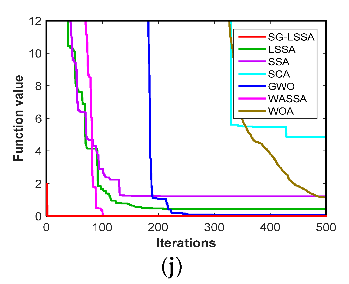
5.3. Testing Results

In

Table 2. Experimental results.

Function	Index	Algorithm
		SG-LSSA	LSSA	SSA	SCA	GWO	WASSA	WOA
F1	Best	1.7149 × 10−8	9.4190 × 10−6	0.0026	2.7607 × 10−4	9.7780 × 10−4	3.4501 × 10−5	3.4089 × 10−7
	Worst	2.9148 × 10−4	0.2208	0.2405	2.4052	1.5090	0.0048	0.5988
	Average	4.2382 × 10−5	0.0371	0.0622	0.2489	0.3093	0.0015	0.0709
F2	Best	5.0676 × 10−7	0.0016	1.1209 × 10−6	6.2883 × 10−4	0.0021	3.8017 × 10−6	5.5204 × 10−6
	Worst	0.0073	0.5839	1.5768	0.2049	2.1918	0.0284	1.8955
	Average	0.0019	0.1171	0.2117	0.0582	0.6822	0.0062	0.5095
F3	Best	0	1.1029 × 10−9	1.1055 × 10−9	4.8778 × 10−51	9.7680 × 10−19	9.6296 × 10−105	2.2145 × 10−62
	Worst	0	4.4637 × 10−7	4.3044 × 10−6	2.7927 × 10−25	1.0946 × 10−7	1.7998 × 10−92	1.2016 × 10−32
	Average	0	1.1609 × 10−7	1.4486 × 10−6	2.8048 × 10−26	1.1041 × 10−8	2.2897 × 10−93	1.2017 × 10−33
F4	Best	0	6.1674 × 10−6	5.1275 × 10−6	5.1451 × 10−65	7.7726 × 10−17	2.0094 × 10−97	7.1086 × 10−140
	Worst	0	0.2989	0.4692	7.2172 × 10−33	0.2050	5.2778 × 10−78	4.5871 × 10−80
	Average	0	0.0553	0.1343	7.8696 × 10−34	0.0205	5.2913 × 10−79	4.5871 × 10−81
F5	Best	−1.0316	−1.0314	−1.0273	−1.0059	−1.0312	−1.0315	−1.0316
	Worst	−1.0303	−0.0184	0.1054	5.6927 × 10−60	−0.0853	−1.0271	−1.0307
	Average	−1.0313	−0.6261	−0.7338	−0.7126	−0.8019	−1.0303	−1.0314
F6	Best	1.1249 × 10−258	0.0014	0.0053	6.9374 × 10−12	1.9604 × 10−4	3.1461 × 10−39	1.1122 × 10−58
	Worst	2.0329 × 10−247	0.0313	0.0581	0.0496	0.0136	2.9003 × 10−37	9.1087 × 10−5
	Average	2.3432 × 10−248	0.0089	0.0292	0.0051	0.0031	8.0385 × 10−38	1.7999 × 10−5
F7	Best	0	4.0577 × 10−12	2.9637 × 10−8	4.3226 × 10−21	3.4116 × 10−20	9.7588 × 10−319	2.1357 × 10−11
	Worst	0	1.0193 × 10−5	8.9379 × 10−4	6.9044 × 10−6	0.0134	1.3363 × 10−261	6.2085 × 10−8
	Average	0	1.0563 × 10−6	1.8866 × 10−4	8.3207 × 10−7	0.0013	1.3363 × 10−262	1.4029 × 10−8
F8	Best	0	5.1896 × 10−6	9.1927 × 10−4	4.0282 × 10−12	3.2142 × 10−6	0	1.8578 × 10−7
	Worst	0	0.0013	0.1304	7.2423 × 10−4	0.0797	0	0.0564
	Average	0	5.3009 × 10−4	0.0239	7.7976 × 10−5	0.0096	0	0.0195
F9	Best	0	0.0074	8.3364 × 10−4	5.1159 × 10−12	8.0696 × 10−5	0	7.9581 × 10−13
	Worst	0	0.6243	3.2526	4.6240	1.6450	0	1.3084 × 10−4
	Average	0	0.1128	0.9956	0.4719	0.2836	0	1.8209 × 10−5
F10	Best	0	0.0323	0.5413	6.5160 × 10−36	3.3546 × 10−5	6.8725 × 10−75	0.0588
	Worst	0	1.2227	2.2829	40.5392	0.4203	3.8488 × 10−72	3.9102
	Average	0	0.4108	1.2020	4.8680	0.0739	1.5327 × 10−72	1.1359

, Best, Worst, and Average mean the optimal function value, the worst function value, and the average value when functions are calculated ten times. We can find that the optimal values calculated by the SG-LSSA are much closer to the ideal values in Table 2, and it is clear to find that the SG-LSSA also can get the best target in high-dimension searching space. Although WASSA also finds the best value in F₈ and F₉, we can see that the iterative capability of WASSA is weaker than that of SG-LSSA in the average convergence curves. SG-LSSA is clearly more stable than WASSA in all iterative curves. In F₅, all values of SG-LSSA are closer to −1.0316. In SG-LSSA, followers use lévy-flight trajectory and the good solution of current iteration to find better solution, and random parameters created by the lévy-flight trajectory can increase the diversity of feasible solutions for continuous nonlinear optimization problems with higher dimensions within shorter computation times compared to the other evolutionary algorithms, which make functions fast convergence to extremum, so SG-LSSA can find exact zero values in F₃, F₄, and F₇–F₁₀. SG-LSSA outperforms all other algorithms in all functions. Therefore, the proposed algorithm has a high performance when finding the global minimum in low-high dimension functions. Table 2 can demonstrate that the SG-LSSA, which is able to provide very competitive results, has a consistent and reliable capacity to find an optimal solution, and its SG-LSSA solving ability is better than that of the LSSA. Hence, SG-LSSA has a better ability than other algorithms to forge the global optimum.

Figure 3 shows the average convergence curves of different algorithms disposing unimodal benchmark functions over 10 independent runs. These figures indicate that SG-LSSA has high stability and is robust compared to other algorithms, and the figures can display the ability of SG-LSSA to escape from poor local optima and get the global optimum. The SG-LSSA has the fastest convergence speed and the best ability to jump out of the local optimum in the last iteration stage when finding the global optimum. SG-LSSA is also able to provide very competitive results on the different benchmark functions. In comparison, other algorithms have poor performances for all functions. The above analysis suggests convinces that the SG-LSSA has an optimal searching performance and the highest searching accuracy.

The box-plot chart, which can express scattered data, is also called the whisker chart. Several samples can be compared by evaluating the maximum value, the minimum value, the median and the upper quartile in the box-plot chart. The performance of algorithms can be analyzed by a box-plot chart. Figure 4 shows the box-plot charts of all algorithms when functions are calculated ten times. Values calculated by the proposed algorithm have the narrowest box-plot charts and fewest outliers in Figure 4. The median, upper quartile, and lower quantile in SG-LSSA box-plot charts are lower than other algorithms, which show that the SG-LSSA has a powerful balance ability when handling different functions. When comparing SG-LSSA box-plot chart and other algorithms box-plots, we can conclude that SG-LSSA performs better with comparison algorithms. Hence, these box-plots can demonstrate that the results of the SG-LSSA are statistically significant, did not occur by coincidence and has merit in terms of exploration.

6. Results and Discussions

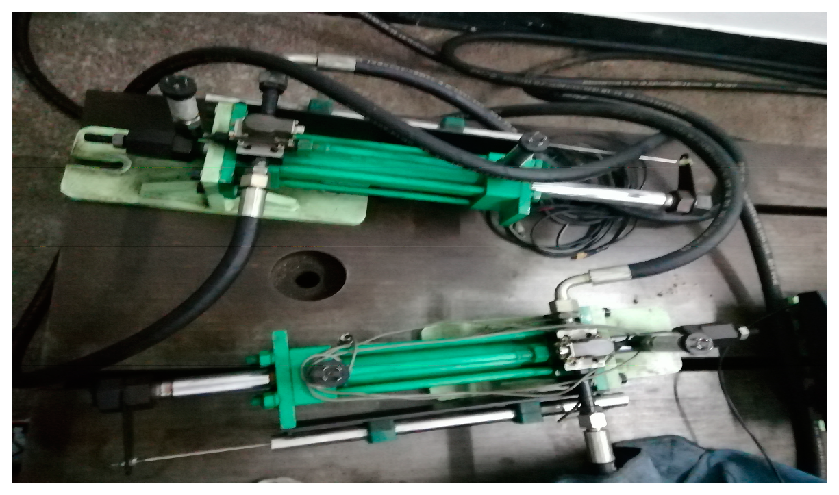
6.1. System Parameters and Working Principle

The system platform is shown in Figure 5. The system platform is the semi-physical simulation platform including a computer, a signal acquisition card, hydraulic oil source, and electro-hydraulic systems. The computer is used to create the real-time signal, adjust the signal value, and handle the collected data from online to offline. The signal acquisition card can be used for processing the analog signal. Electro-hydraulic systems mainly consist of an actuator cylinder, force sensor, the piston rod, sliding guide rail, load, inertial load, and flexible link, and so on. When the system platform is operated, the real-time signal generated by the computer is input into the servo amplifier through the A/D signal acquisition card, then, the amplified signal is transmitted into the servo valve as the driving signal to control the movement of the hydraulic cylinder piston rod. At the same time, the force sensor inputs the detected force signal into the computer through the A/D signal acquisition card to complete the servo. The electro-hydraulic servo valve is an FF102-30 (AVIC Nanjing Servo Control System Co., Ltd., Nanjing, China). Platform parameters in this paper were obtained in different ways, including maintenance and instrumentation manuals, engineering experience, testing experiments, and numerical calculation. The current saturation value 40 (mA) to 50 (mA). Inlet oil pressure 21 (MPa). Rated flow 30 (L/min). Piston Diameter 50 (mm). Piston rod diameter 35 (mm). The voltage saturation value −10 (V) to 10 (V). Oil supply pressure 5 (MPa). In practical engineering problems, due to complexities of the structure control, the influence of temperature, the density of hydraulic oil, inaccurate measurements, and other factors, it is difficult to evaluate the stick-slip phenomena by building the precise mathematical model. All testing experiments of this paper were carried out in the same environment, and the main purpose of this paper is to keep the stick-slip phenomenon as similar as possible.

To show the performance of the proposed PID controller, this paper carried out the comparative PID controllers in MATLAB. Different algorithms used in PID controllers include SF-LSSA, LSSA, SSA, SCA, GWO, WASSA, and WOA. Parameters applied in the results are determined according to the test function environment. The range of PID parameters were generated in [0, 100]. Discrete ITSE was selected as the evaluation function. Set maximum iterations 500. Set population size 100. The sampling period was selected as 100 and 0.01 s. Each algorithm was implemented in the MATLAB software (MathWorks, Natick, MA, USA).

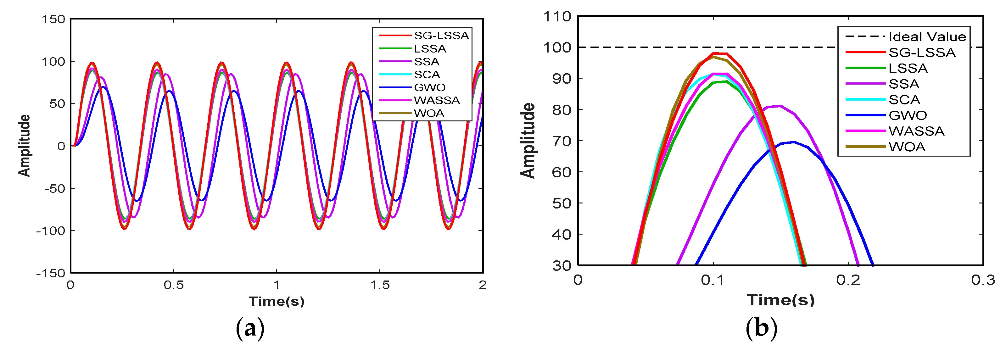
6.2. Temporal Response Characteristic

Table 3. Proportional–integral–derivative (PID) parameters and temporal response characteristic.

Parameters	Algorithm
	SG-LSSA	LSSA	SSA	SCA	GWO	WASSA	WOA
KP	2.2980	2.6097	0.1011	3.1793	0	2.6767	2.6391
Ki	100	72.9233	41.4366	80.5416	29.3905	81.9920	92.2762
Kd	0.0111	0.0117	0.0038	0	0	0.0128	0
ITSE	3.7329 × 10−6	4.4337 × 10−6	1.7682 × 10−5	4.7062 × 10−6	2.8424 × 10−5	4.0253 × 10−6	4.4170 × 10−6
Mp	0.0236	0	0.0521	0.1276	0.0091	0	0.1182
ts	0.08	0.16	0.25	0.17	0.20	0.13	0.11
tp	0.05	1	0.19	0.05	0.28	1	0.06
td	0.03	0.03	0.07	0.04	0.09	0.03	0.04
er	3.9733 × 10−12	1.6479 × 10−9	1.901 6× 10−8	1.5339 × 10−8	1.4850 × 10−9	4.9603 × 10−11	1.2672 × 10−11

shows the PID parameters, ITSE, and temporal response indices. A class of nonlinear time-varying processes of the system output is called the system temporal response under the condition of step signal. The system temporal response can be divided into the transient response and the steady-state response. The transient response reverses the reliability and the regulation accuracy, including overshoot Mp, delay time t_d, peak time t_p, and settling time t_s. Overshoot indicates the difference in value between the maximum output signal and the ideal output signal. Peak time means that the operation time makes the working signal reach a maximum. Delay time indicates the running time from the output signal to the half-steady state. Settling time means the running time that makes the output signal keep within a ±2% steady-state error range. The steady-state response index e_r, which reflects the balance and damping of the system, is the difference between the ideal stable state and the stable output state. The SG-LSSA parameter-tuning method has the lowest temporal response indices, and the smallest ITSE of all algorithms, which show the superior performance of the proposed SG-LSSA-PID controller. Although the overshoot of the LSSA-PID controller is equal to zero, it takes a long time for the system to reach the peak time and stable state, which increases system consumption and damages the system. The system using the proposed controller can keep excellent tracking transformation characteristics and a fast-driving speed. These results identify that the SG-LSSA-PID controller possesses the best temporal response performance.

The response curves two-dimensional graph and three-dimensional graph are shown in Figure 6. The response curve of the system controlled by the SG-LSSA-PID controller converges to the ideal steady-state with the optimum overshoot. The overshoot of the system controlled by SCA-PID has the maximum overshoot. Response curves of the system that are controlled by the SSA-PID and GWO-PID have too large running time, which can cause system high pressure and deterioration. The WASSA-PID controller and LSSA-PID controller need to run a long time to arrive at the ideal value. Although the SG-LSSA-PID controller has a small amount of overshoot, it jumps right back into the ideal value. When the SCA-PID controller and WOA-PID controller have maximum overshoot, they have a violent shock. Using the SG-LSSA-PID controller, the system can retain high precision validity, and the system performance is a small impact on outside time-varying signals, displaying high availability, fine maintainability.

The ITSE iteration curve and the ITSE box plot are shown in Figure 7. The ITSE iteration curve indicates that SG-LSSA has the highest searching speed in all algorithms, which shows the best optimization capability when tuning PID parameters. The SG-LSSA convergence curve rapidly accelerates in the early iterations and quickly tracks the minimum ITSE after half-stage iterations, which further demonstrates that SG-LSSA has great optimization efficiency and ability to jump out from local optimum. The box plot displays the system stability by calculating the ITSE graphical dispersion. ITSE calculated by SG-LSSA-PID has the smallest outlier and the lowest dispersion degree in all algorithms, which demonstrate that the SG-LSSA-PID has an outstanding balance. The results further confirm that SG-LSSA has perfect searching optimization capability.

6.3. The Frequency Response Characteristic

The frequency response, which can evaluate abilities to reproduce signals and filtering the noise in systems, is the system response under sinusoidal signals. The amplitude-frequency characteristic is defined as the ratio of the actual amplitude to the ideal amplitude. If the actual amplitude is closer to the ideal amplitude, the system is more stable. To further prove the perfect mechanical impedance and dynamic stiffness of the SG-LSSA-PID controller, four sinusoidal signals were entered into controlled systems. For different sinusoidal signals, the angular velocities were respectively set as 10 and 20, and when the initial phase was zero, the amplitude was set to 1, 50, and 100. The response results and the local amplification are presented in Figure 8, Figure 9, Figure 10, Figure 11, Figure 12 and Figure 13. As we can see in these figures, the system controlled by GWO-PID has the maximum amplitude difference between the output amplitude and the ideal amplitude. Local enlarged drawings for the SG-LSSA-PID controller are closest to the ideal amplitude. Figure 8, Figure 9, Figure 10, Figure 11, Figure 12 and Figure 13 clearly show that the SG-LSSA-PID controller can not only rapidly restrain interfering signals but also improve accuracy tracking. For input signals combined with noise and interference, the proposed controller has a perfect ability to maintain reliable inspection and reduce nonlinear error. Therefore, we can deduce that the SG-LSSA-PID controller has anti-seismic properties and vibration stability in the unknown interference environments.

7. Conclusions

In this paper, a self-growing lévy-flight salp swarm algorithm has been proposed and used in PID controllers to increase the stability and of PID controllers. The proposed SG-LSSA-PID controller, whose parameters are tuned by SG-LSSA, is applied to the force actuator system to enhance the real-time system performance. The actuator force control system model was established, and the transfer function model was calculated. To demonstrate the searching effectiveness of the proposed SG-LSSA, ten benchmark functions were tested and compared with other algorithms. Then, the performance of the system controlled by the SG-LSSA PID controller was estimated by calculating ITSE. Finally, this paper analyzed the temporal response characteristic and the frequency response characteristic. The results show that the system driven by the SG-LSSA PID controller has high practicability, good accuracy, and strong robustness in unknown environments.

References

1. Kilic, E.; Dolen, M.; Koku, A.B.; Caliskan, H.; Balkan, T. Accurate pressure prediction of a servo-valve controlled hydraulic system. Mechatronics 2012, 22, 997–1014. [Google Scholar] [CrossRef]
2. Lin, A.; Sun, Y.; Zhang, H.; Lin, X.; Yang, L.; Zheng, Q. Fluctuating characteristics of air-mist mixture flow with conjugate wall-film motion in a compressor of gas turbine. Appl. Therm. Eng. 2018, 142, 779–792. [Google Scholar] [CrossRef]
3. Xu, B.; Chen, D.; Tolo, S.; Patelli, E.; Jiang, Y. Model validation and stochastic stability of a hydro-turbine governing system under hydraulic excitations. Int. J. Electr. Power Energy Syst. 2018, 95, 156–165. [Google Scholar] [CrossRef] [Green Version]
4. Lin, A.; Zheng, Q.; Jiang, Y.; Lin, X.; Zhang, H. Sensitivity of air/mist non-equilibrium phase transition cooling to transient characteristics in a compressor of gas turbine. Int. J. Heat Mass Transf. 2019, 137, 882–894. [Google Scholar] [CrossRef]
5. Nguyen, M.T.; Dang, T.D.; Ahn, K.K. Application of Electro-Hydraulic Actuator System to Control Continuously Variable Transmission in Wind Energy Converter. Energies 2019, 12, 2499. [Google Scholar] [CrossRef] [Green Version]
6. Xia, L.; Quan, L.; Ge, L.; Hao, Y. Energy efficiency analysis of integrated drive and energy recuperation system for hydraulic excavator boom. Energy Conv. Manag. 2018, 156, 680–687. [Google Scholar] [CrossRef]
7. Jia, X.; Zhang, H.; Zheng, Q. Numerical investigation on the effect of hot running rim seal clearance on hot gas ingestion into rotor-stator system. Appl. Therm. Eng. 2019, 152, 79–91. [Google Scholar] [CrossRef]
8. Gao, B.; Shao, J.; Yang, X. A compound control strategy combining velocity compensation with ADRC of electro-hydraulic position servo control system. ISA Trans. 2014, 53, 1910–1918. [Google Scholar] [CrossRef] [PubMed]
9. Guo, Q.; Zhang, Y.; Celler, B.G.; Su, S.W. State-Constrained Control of Single-Rod Electrohydraulic Actuator with Parametric Uncertainty and Load Disturbance. IEEE Trans. Control Syst. Technol. 2018, 26, 2242–2249. [Google Scholar] [CrossRef]
10. Sun, C.; Fang, J.; Wei, J.; Hu, B. Nonlinear Motion Control of a Hydraulic Press Based on an Extended Disturbance Observer. IEEE Access 2018, 6, 18502–18510. [Google Scholar] [CrossRef]
11. Yang, Y.; Li, G.; Zhang, Q. A Pressure-Coordinated Control for Vehicle Electro-Hydraulic Braking Systems. Energies 2018, 11, 2336. [Google Scholar] [CrossRef] [Green Version]
12. Shen, G.; Zhu, Z.-C.; Li, X.; Tang, Y.; Hou, D.-D.; Teng, W.-X. Real-time electro-hydraulic hybrid system for structural testing subjected to vibration and force loading. Mechatronics 2016, 33, 49–70. [Google Scholar] [CrossRef]
13. Kallu, K.; Wang, J.; Abbasi, S.; Lee, M. Estimated Reaction Force-Based Bilateral Control between 3DOF Master and Hydraulic Slave Manipulators for Dismantlement. Electronics 2018, 7, 256. [Google Scholar] [CrossRef] [Green Version]
14. Guo, Q.; Wang, Q.; Li, X. Finite-Time Convergent Control of Electrohydraulic Velocity Servo System Under Uncertain Parameter and External Load. IEEE Trans. Ind. Electron. 2019, 66, 4513–4523. [Google Scholar] [CrossRef]
15. Jiangbo, Z.; Junzheng, W. The fractional order PI control for an energy saving electro-hydraulic system. Trans. Inst. Meas. Control 2015, 39, 505–519. [Google Scholar] [CrossRef]
16. Han, J. From PID to Active Disturbance Rejection Control. IEEE Trans. Ind. Electron. 2009, 56, 900–906. [Google Scholar] [CrossRef]
17. Valério, D.; da Costa, J.S. Tuning of fractional PID controllers with Ziegler–Nichols-type rules. Signal Process. 2006, 86, 2771–2784. [Google Scholar] [CrossRef]
18. Das, J.; Mishra, S.K.; Saha, R.; Mookherjee, S.; Sanyal, D. Nonlinear modeling and PID control through experimental characterization for an electrohydraulic actuation system: system characterization with validation. J. Braz. Soc. Mech. Sci. Eng. 2016, 39, 1177–1187. [Google Scholar] [CrossRef]
19. Padula, F.; Visioli, A. Tuning rules for optimal PID and fractional-order PID controllers. J. Process Control 2011, 21, 69–81. [Google Scholar] [CrossRef]
20. Nedic, N.; Prsic, D.; Dubonjic, L.; Stojanovic, V.; Djordjevic, V. Optimal cascade hydraulic control for a parallel robot platform by PSO. Int. J. Adv. Manuf. Technol. 2014, 72, 1085–1098. [Google Scholar] [CrossRef]
21. Essa, M.E.-S.M.; Aboelela, M.A.S.; Hassan, M.A.M. Position control of hydraulic servo system using proportional-integral-derivative controller tuned by some evolutionary techniques. J. Vib. Control 2014, 22, 2946–2957. [Google Scholar] [CrossRef]
22. Wang, R.; Tan, C.; Xu, J.; Wang, Z.; Jin, J.; Man, Y. Pressure Control for a Hydraulic Cylinder Based on a Self-Tuning PID Controller Optimized by a Hybrid Optimization Algorithm. Algorithms 2017, 10, 19. [Google Scholar] [CrossRef] [Green Version]
23. Fan, Y.; Shao, J.; Sun, G. Optimized PID Controller Based on Beetle Antennae Search Algorithm for Electro-Hydraulic Position Servo Control System. Sensors 2019, 19, 2727. [Google Scholar] [CrossRef] [Green Version]
24. Li, C.; Mao, Y.; Zhou, J.; Zhang, N.; An, X. Design of a fuzzy-PID controller for a nonlinear hydraulic turbine governing system by using a novel gravitational search algorithm based on Cauchy mutation and mass weighting. Appl. Soft. Comput. 2017, 52, 290–305. [Google Scholar] [CrossRef]
25. Mirjalili, S.; Gandomi, A.H.; Mirjalili, S.Z.; Saremi, S.; Faris, H.; Mirjalili, S.M. Salp Swarm Algorithm: A bio-inspired optimizer for engineering design problems. Adv. Eng. Softw. 2017, 114, 163–191. [Google Scholar] [CrossRef]
26. Gao, H.; Hou, Y.; Zhang, S.; Diao, M. An Efficient Approximation for Nakagami-m Quantile Function Based on Generalized Opposition-Based Quantum Salp Swarm Algorithm. Math. Probl. Eng. 2019, 2019, 1–13. [Google Scholar]
27. Hasanien, H.M.; El-Fergany, A.A. Salp swarm algorithm-based optimal load frequency control of hybrid renewable power systems with communication delay and excitation cross-coupling effect. Electr. Power Syst. Res. 2019, 176, 105938. [Google Scholar] [CrossRef]
28. Ali, T.A.A.; Xiao, Z.; Sun, J.; Mirjalili, S.; Havyarimana, V.; Jiang, H. Optimal design of IIR wideband digital differentiators and integrators using salp swarm algorithm. Knowl.-Based Syst. 2019, 182, 104834. [Google Scholar] [CrossRef]
29. Zhang, J.; Wang, Z.; Luo, X. Parameter Estimation for Soil Water Retention Curve Using the Salp Swarm Algorithm. Water 2018, 10, 815. [Google Scholar] [CrossRef] [Green Version]
30. Wang, J.; Gao, Y.; Chen, X. A Novel Hybrid Interval Prediction Approach Based on Modified Lower Upper Bound Estimation in Combination with Multi-Objective Salp Swarm Algorithm for Short-Term Load Forecasting. Energies 2018, 11, 1561. [Google Scholar] [CrossRef] [Green Version]
31. Jumani, T.A.; Mustafa, M.; Anjum, W.; Ayub, S. Salp Swarm Optimization Algorithm-Based Controller for Dynamic Response and Power Quality Enhancement of an Islanded Microgrid. Processes 2019, 7, 840. [Google Scholar] [CrossRef] [Green Version]
32. Xing, Z.; Jia, H. Multilevel Color Image Segmentation Based on GLCM and Improved Salp Swarm Algorithm. IEEE Access 2019, 7, 37672–37690. [Google Scholar] [CrossRef]
33. Jamil, M.; Yang, X. A literature survey of benchmark functions for global optimisation problems. Int. J. Math. Model. Numer. Optim. 2013, 4, 150–194. [Google Scholar] [CrossRef] [Green Version]
34. Yang, X. Test problems in optimization. arXiv 2010, arXiv:1008.0549. Available online: https://arxiv.org/pdf/1008.0549.pdf (accessed on 16 January 2020).
35. Mirjalili, S. SCA: A Sine Cosine Algorithm for solving optimization problems. Knowl.-Based Syst. 2016, 96, 120–133. [Google Scholar] [CrossRef]
36. Mirjalili, S.; Mirjalili, S.M.; Lewis, A. Grey Wolf Optimizer. Adv. Eng. Softw. 2014, 69, 46–61. [Google Scholar] [CrossRef] [Green Version]
37. Wu, J.; Nan, R.; Chen, L. Improved salp swarm algorithm based on weight factor and adaptive mutation. J. Exp. Theor. Artif. Intell. 2019, 31, 493–515. [Google Scholar] [CrossRef]
38. Mirjalili, S.; Lewis, A. The Whale Optimization Algorithm. Adv. Eng. Softw. 2016, 95, 51–67. [Google Scholar] [CrossRef]
Figure 1. The force controlled the electrohydraulic system. (a) The system structure diagram; (b) the simplified working principle diagram.
Energies 13 00459 g001
Figure 2. The flow chart of tuning steps.
Energies 13 00459 g002
Figure 3. The average convergence curves. (aj) Function 1–10.
Energies 13 00459 g003aEnergies 13 00459 g003b
Figure 4. The box-plot charts. (aj) Function 1–10.
Energies 13 00459 g004aEnergies 13 00459 g004b
Figure 5. The system platform.
Energies 13 00459 g005
Figure 6. The step response curves. (a) The two-dimensional graph; (b) the three-dimensional graph.
Energies 13 00459 g006
Figure 7. The integral of time multiplied by the square value of error (ITSE) iteration curve and the ITSE box plot. (a) The ITSE iteration curve; (b) the ITSE box plot.
Energies 13 00459 g007
Figure 8. The frequency response of amplitude 1 and angular velocity 10. (a) The response curve; (b) local amplification.
Energies 13 00459 g008
Figure 9. The frequency response of amplitude 50 and angular velocity 10. (a) The response curve; (b) local amplification.
Energies 13 00459 g009
Figure 10. The frequency response of amplitude 100 and angular velocity 10. (a) The response curve; (b) local amplification.
Energies 13 00459 g010
Figure 11. The frequency response of amplitude 1 and angular velocity 20. (a) The response curve; (b) local amplification.
Energies 13 00459 g011
Figure 12. The frequency response of amplitude 50 and angular velocity 20. (a) The response curve; (b) local amplification.
Energies 13 00459 g012
Figure 13. The frequency response of amplitude 100 and angular velocity 20. (a) The response curve; (b) local amplification.
Energies 13 00459 g013