Article

Is Investing in Companies Manufacturing Solar Components a Lucrative Business? A Decision Tree Based Analysis

by
Sebastian Klaudiusz Tomczak
1,*,
Anna Skowrońska-Szmer
1 and
Jan Jakub Szczygielski
2,3
1
Department of Operations Research and Business Intelligence, Wrocław University of Science and Technology, Wyspiańskiego 27, 50-370 Wrocław, Poland
2
Department of Financial Management, University of Pretoria, Pretoria 0002, South Africa
3
Newcastle Business School, Northumbria University, Newcastle NE1 8ST, UK
*
Author to whom correspondence should be addressed.
Energies 2020, 13(2), 499; https://doi.org/10.3390/en13020499
Submission received: 28 November 2019 / Revised: 9 January 2020 / Accepted: 15 January 2020 / Published: 20 January 2020
(This article belongs to the Special Issue Economics of Sustainable and Renewable Energy Systems)

Abstract

:
In an era of increasing energy production from renewable sources, the demand for components for renewable energy systems has dramatically increased. Consequently, managers and investors are interested in knowing whether a company associated with the semiconductor and related device manufacturing sector, especially the photovoltaic (PV) systems manufacturers, is a money-making business. We apply a new approach that extends prior research by applying decision trees (DTs) to identify ratios (i.e., indicators), which discriminate between companies within the sector that do (designated as “green”) and do not (“red”) produce elements of PV systems. Our results indicate that on the basis of selected ratios, green companies can be distinguished from the red companies without an in-depth analysis of the product portfolio. We also find that green companies, especially operating in China are characterized by lower financial performance, thus providing a negative (and unexpected) answer to the question posed in the title.

Graphical Abstract

1. Introduction

The majority of the global energy supply is generated by the burning of fossil fuels. Progress and global economic growth have been accompanied by an increase in the consumption of fossil fuels, resulting in climate change and global warming. Importantly, fossil fuels are distributed unequally across the global geography, creating challenges related to access in unstable and conflict zones. This has resulted in a shift towards the use of renewable energy sources (RES), with the intention of reducing dependency on fossil fuels and the challenges associated with the use of fossil fuels. Renewable energy is locally available, clean, sustainable and eco-friendly and therefore offers an attractive alternative to fossil fuels. Consequently, researchers and policy makers have shown an increased interest in greener sources of energy. According to data [1] available from the International Energy Agency (IEA), the share of electricity generation from renewable sources in overall energy production in 2018 has exceeded 25% and is constantly growing. This is evident in the increased production numbers of renewable energy over the three preceding decades (see Figure 1). During recent decades, the share of energy from wind and solar photovoltaic (PV) in total production of renewable energy has increased significantly.
Many countries have decided to promote renewable energy and to reduce dependence on fossil fuels and to do so, have established mandatory renewable energy targets. Such measures form part of respective governments’ legislated plans that require electricity retailers to source specific proportions of total electricity sales from RES within a fixed time frame. For example, the People’s Republic of China and India have a target level of 50% and 40% of total electric power generation from non-fossil energy sources, respectively. Renewable energies have been incorporated leading source of non-fossil energy. Specifically, the People’s Republic of China has established targets of 723 GW from RES by 2020. The underlying targets include increasing wind power capacity to 210 GW and solar energy to 110 GW [2]. In turn, the government of India set a target of achieving 175 GW from RES by 2022 which mainly consists of energy from solar (100 GW) and wind (60 GW) [3]. Moreover, Turkey, Thailand and Chinese Taipei have established RES targets as part of their total electric power generation. Turkey has set a target share of RES at 30% by 2030. Thailand has set a target level of 20% by 2036 and Chinese Taipei has a target of 8% by 2025 (see Figure 2). According to data provided by the IEA, none of the countries with set targets have achieved their targets, aside from Turkey which achieved its target in 2015.
Achieving these targets necessitates an increase in installed electric power generation capacity. Thus, the demand for manufactured solar modules, solar cells, solar silicon rods, solar wafers, solar power, solar photovoltaic products and equipment is increasing. This increase in demand is further compounded by the incentives offered by governments to promote investment in the PV industry and RES energy in general. For example, the Chinese government has set up national science and technology plans to support the research and development (R&D) into PV technology, the setting up of key laboratories that promote R&D in the industry and the promotion of demonstration projects in rural areas. Also, a feed-in tariff policy was implemented and exemptions from import tariffs were offered for imported equipment for domestic and foreign PV investment projects. The Chinese government also offered tax incentives for PV related enterprises in the form of R&D cost rebates, rebates for the purchases of special equipment and the amortization of costs for intangible assets and tax policies to promote PV power generation, high-tech enterprises in the PV sector and investment in R&D and PV production processes [7,8] provides an overview of the measures applied to promote investment in PV capacity within the EU-27 countries. The most popular measure to promote PV is the use of feed-in tariffs, which guarantee the price at which electricity is purchased. This is then followed by subsidies which are part of specific national programmes although subsidies are decreasing. Then, tax incentives are offered in almost half of the EU-27 countries. Broadly, these include tax credits, exemptions and reduced tax rates. For example, in Bulgaria, value added tax (VAT) for PV revenues is 10% as opposed to the normal rate of 15%. Tax deductions or tax credits are applied in Belgium, Denmark, France, Germany, Ireland and the Netherlands, reducing the amount of taxable income or the amount of tax due respectively. A number of countries have implemented tradable green certificates. For example, Belgium implemented a green certificate trading system for electricity, providing renumeration per certificate coming from a grid operator. Finally, soft loans have also been offered by a small number of EU countries. Solangi et al. [9] outline measures used to promote solar energy deployment in the US and Canada. In the US, incentives were formulated as early as 1978, with investment tax credits being offered for renewable energy technologies initially. Residential tax credits of 30% and business tax credits for investment in renewable energy, including solar energy, of 15% were offered respectively. Later on, residential and business investment tax credits were raised to 30% and extended, resulting in a doubling of installed PV capacity. In Canada, feed-in tariffs were implemented in 18 provinces, with the feed-in tariff implemented in Ontario credited with stimulating manufacturing and the growth of the Ontario PV industry. The Canadian government also provided loan guarantees, tax holidays and subsidies to support PV manufacturing. Sachu [10] outlines policies applied in the top 10 RES producing countries, including Germany. To promote the use of renewable energy, the German government mandated the purchase of renewable energy and offered large subsidies to renewable energy producers. A target was set to reach a specified level of solar PV capacity and feed-in tariffs were established. Sachu [10] notes that the policies applied in Germany have had a significant impact on reducing soft costs associated with solar installation, such as permitting, inspections, interconnection, financing and customer acquisition.
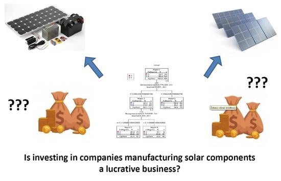
All these policies, which include targets and incentives, require that investment in RES companies increases. This can readily take place happen if RES related companies, specifically those that produce photovoltaic components, offer an attractive alternative to other companies that belong to the semiconductor and related device manufacturing sector and are lucrative overall. We contribute to the literature on RES by focusing on a class of companies that operate within the renewable energy value chain. These are companies that manufacture semiconductors and related solid state devices. We divide these companies into two groups. The green group comprises companies that manufacture solar modules, solar cells, solar silicon rods, solar wafers, solar power, solar photovoltaic products and related equipment for RES companies. This group is the focus of this paper. The red group comprises the remainder of companies that are not associated with RES companies).
We seek to identify ratios (i.e., indicators), which discriminate between companies within the manufacturing sector that produce PV components and those that do not. Once we have identified such ratios, we can analyze these ratios to answer the question as to whether these companies show strong financial performance, that is, offer an attractive investment alternative. In the literature, there is great interest in evaluating returns for the energy sector, especially for companies that produce renewable energy. Relationships between returns on renewable energy stocks, changes in the oil price, equity indices, carbon prices and carbon pass-through rates, for example, Trück and Weron [11] examine convenience yields and risk premiums in the EU-wide CO2 emissions trading scheme during the first Kyoto commitment period. They report that during their sample period, the EUA market has shifted from a period of backwardation to a period of contango with negative convenience yields. Bohl et al. [12] investigate the common factors driving the performance of German renewable energy stocks. They find that renewable energy stocks mirror ambiguity related to the future economic outlook faced by the industry. Henriques and Sadorsky [13] investigate the relationship between alternative energy stock prices, technology stock prices, oil prices and interest rates. Stock prices for alternative energy companies are found to be impacted by shocks to technology stock prices but shocks to oil prices do not have an impact on alternative energy companies. Inchauspe et al. [14] investigate the impact of energy prices and stock market indices on private investments in renewable energy, finding that these have shown substantial growth attributable to government policies, oil prices and evolving market liquidity. Kumar et al. [15] analyze the relationship between oil prices and alternate energy prices, finding that oil prices, stock prices for high technology firms and interest rates impact clean stocks. Managi and Okimoto [16] analyze the relationships between oil prices, clean energy stocks prices and technology stock prices. The impact of legislation on electricity future contracts in examined by Reference [17]. Studies also investigate the financial performance of firms operating in the energy sector [18,19,20,21,22]. For example, Capece et al. [18] focus on changes in the performance of the natural gas retail markets and analyze the financial statements of 105 companies by performing cluster analysis. They report that most companies in the sector perform well, with best performers belonging to existing business groups. Capece et al. [19] analyze the combined effect of regulatory measures and of the economic crisis on the performance of Italian gas companies. The observe that average measures of profitability rose until 2009 and then declined in 2009. This is attributed to the financial crisis and regulatory policies.
A number of studies, similarly to ours, evaluate the financial performance of firms that operate within the renewable energy sector using financial ratios. For example, Halkos and Tzeremes [20] evaluate the financial performance of renewable energy firms. They apply a data envelopment analysis and construct financial ratios to assess performance. Performance is found to be positively related to high levels of returns on assets and equity and by lower levels of debt. They also undertake a within sector analysis, finding that firms producing wind energy outperform firms generating hydropower. The dataset is limited to the Greek renewable energy sector and considers a limited number of ratios in the analysis of RES firm performance. Paun [21] analyzes the sustainability of the renewable energy sector in Romania. Their sample encompasses 91 major energy producers for the years 2012 to 2015. To analyze performance, they consider profitability ratios, measures of return on equity and measures of return on assets but do not consider key measures in the form of return on investment and the current ratio, given limitations in the data. They find that companies that produce fossil fuels perform better relatively to companies that produce green energy. They also report deteriorating performance, after 2013 and relatively low returns on equity for RES firms after 2014, suggesting that RES firms underperform other sectors. Also, returns on assets are found to decrease after 2013, this being attributed to changes in government and delays in issuing green certificates, leading to decreases in investment. Based upon ratio analysis, Paun [21] concludes that RES companies are close to financial distress. Tomczak [22] investigates whether powerplants that produce electricity using renewable energy sources are in a better financial position than those that rely upon traditional (fossil fuel) energy sources using a sample of companies in Baltic and Central European countries, comprising a total sample of 37 companies. In order to assess financial performance, he considers a total of 16 ratios indicative of four aspects, namely liquidity, profitability, turnover and debt—ratios that are used in bankruptcy prediction. An analysis of ratios shows RES companies have lower return on assets and return on equity ratios than fossil fuel energy producers, which translates into lower interest from potential investors. Also, fossil fuel companies were found to be characterized by higher profitability but lower turnover ratios. Tomczak [22] concludes that investing in RES companies is not profitable business. Our study is similar to these studies; we also consider financial ratios, through the use of DTs, we identify and then analyze financial ratios to gain an insight into the performance of green companies.
Another strand of literature considers the relationship between corporate environmental performance and financial performance, with performance again measured by ratios, demonstrating the value of ratio analysis [23,24,25,26]. Clarkson et al. [23] investigate the factors that impact firms’ decisions to engage in a proactive environmental strategy. The study is carried out using a sample of firms belonging to the four most polluting firms in the US, namely the pulp and paper, chemical, oil and gas and metals and mining industries. They consider how changes in environmental strategy impact profitability, liquidity and leverage. Analysis shows that becoming green leads to improved firm performance and that improved firm performance subsequently improves relative environmental performance. This is reflected by increasing return on assets, rising cashflows (profitability) and a decreases in leverage. Ruggiero and Lehkonen [24] show that there is a negative relationship between renewable energy production by electricity producers and short- and long-term financial performance. To measure financial performance, they use the return on equity and the return on assets and a firm’s market value relative to total assets and regress these onto the volume of renewable energy produced, as a main variable of interest. Granger-causality is also tested. They find a negative relationship between measures of financial performance and the amount of renewable energy produced, attributing this to higher capital costs. Sueyoshi and Goto [25] examine the impact of environmental regulations in the US. Similarly to Ruggiero and Lehkonen [24], they use the return on assets as a measure of financial performance. They regress the return on assets for a 167 US electric utilities onto measures of environmental protection. Results indicate that environmental protection expenditure by US electric utilities has resulted in decreased financial performance. Sueyoshi and Goto [25] conclude that that both the positive and negative aspects of environmental policies should be considered, given that emphasis is usually placed upon the positive aspects and negative aspects. Telle [26] challenges the methods applied in previous studies to conclude that firms that go green benefit financially. They note that one of the issues in studies that seek to relate financial performance to environmental performance is the presence of omitted variables. The omission of variables may result in an (erroneous) positive relationship between financial performance and environmental performance. Telle [26] shows that when the return on sales for Norwegian plants are regressed onto observable firm characteristics and omitted unobserved variables are controlled form, the positive impact of good environmental performance disappears. The study’s significance lies in challenging findings of a positive impact of environmental performance on financial performance. The question of going green—and analogously—of producing components for the RES industry remains unanswered. Within the context of our present study, such findings suggest that green firms—and those related to RES—may not be characterized by improved financial performance relative to firms that are not green.
Finally, a number studies consider further aspects of the financial performance of firms that operate within the energy sector. For example, Pätäri et al. [27] investigate whether corporate social responsibility investments have an impact on corporate performance within the energy industry, finding that different aspects of corporate social responsibility impact either both profitability and/or market value. Arslan-Ayaydin and Thewissen [28] compare the financial performance of energy sector firms with different environmental scores, finding that those with good scores outperform financially those with poor scores. Sueyoshi and Goto [29] investigate the efficiency of national oil companies and aim to establish whether companies that are under public ownership outperform those under international ownership, showing that companies under national ownership outperform international oil companies under international private ownership in terms of efficiency.
None of these studies seek to investigate whether investing in companies manufacturing solar components is a lucrative business by classifying companies on the basis of ratios and then analyzing these ratios. To answer to this question, we apply a decision tree based analysis. We frame our analysis within the theoretical basis provided by literature on corporate failure and financial distress, which relies upon the classification of firms, as we do in this study [30,31]. The genesis of bankruptcy prediction models, is attributed to Beaver (1966) who uses 30 grouped ratios and information for failed and non-failed industrial firms to identify five ratios predictive of bankruptcy. His noteworthy conclusion is that ratios for distressed firms differ from those of healthy firms, making it possible to predict financial distress by discriminating between healthy and distressed firms. Altman [32] builds upon Beaver’s [33] work and applies multiple discriminant analysis (MDA) to estimate a five-factor model predictive of bankruptcy for a sample of manufacturing firms. The joint consideration of ratios in Altman (1968) removes the ambiguity and confusion associated with interpreting individual ratios. Ohlson [34] proposes the use of logit analysis (logistic regression) to estimate an O-score model that combines financial ratios and indicators, yielding a probability of bankruptcy bounded between 0 and 1. The model provides a more precise and readily understood indication of the likelihood of bankruptcy and permits a greater range of outcomes than Altman’s (1968) model. Frydman, Altman and Kao [35] propose a non-parametric solution in the form of decision trees (DTs) to classify distressed and non-distressed firms. DTs require no distributional assumptions or transformed variables. They can handle missing values and qualitative data, are readily understood and can incorporate misclassification costs. They apply these to manufacturing and retailing companies, finding that DTs are more accurate and minimize misclassification costs. Koh and Low [36] show that DTs outperform logit analysis and artificial neural networks in predicting bankruptcies. Similarly, Li, Sun and Wu [37] assess the performance of algorithmic implementations of decision trees for companies on the Shenzen and Shanghai Stock Exchange, finding that these outperform other classifications methods—notably methods used in bankruptcy prediction. Gepp, Kumar and Bhattacharya [38] take a similar approach, showing that DT implementations are superior classifiers and predictors of bankruptcy for retailing and manufacturing companies. Fedorova, Gilenko and Dovzhenko [39] extend the application of bankruptcy prediction models to the Russian manufacturing sector by combining statistical methods with artificial intelligence techniques.
We build upon bankruptcy prediction literature that applies DTs to classify bankrupt firms and to predict bankruptcy. We apply DTs in a novel manner. While we do not aim to predict bankruptcy on the basis of financial ratios, we set out to determine whether companies that manufacture solar modules, solar cells, solar silicon rods, solar wafers, solar power, solar photovoltaic products and related equipment (green companies) can be differentiated from other enterprises in the sector that are not associated with RES companies (red companies) on the basis of financial ratios and whether these companies are in a better financial state. Based upon our analysis, the most critical ratios can be identified from a total of 62 ratios. It is hoped that using these ratios will give managers and investors the ability to undertake a broader and more detailed assessment of companies in the sector, without only focusing on profitability ratios.

2. Data and Methodology

Our methodology comprises a number of steps. First, we collect data from financial reports for companies in the semiconductor and related device manufacturing sector. Financial reports are downloaded from the Emerging Markets Information Service (EMIS) database, a Euromoney Institutional Investor Company (www.emis.com). The initial sample consists of 2345 companies operating in China (1742), Chinese Taipei (272), South Korea (114), Thailand (48), Singapore (37), India (33), Vietnam (24), Hong Kong (21), Malaysia (20), Russia (10), Turkey (6), Ukraine (4), Ecuador (3) and two companies each from the Czech Republic, Indonesia, Iran, Philippines as well as one each from Bulgaria, El Salvador and Romania. To determine whether investing in companies that manufacture RES components pays off, we divide companies in the sector into two groups. The first group comprises enterprises that manufacture solar modules, solar cells, solar silicon rods, solar wafers, solar power, solar photovoltaic products and related equipment. We define companies within this group as green companies. The second group comprises companies that are not associated with RES companies. We defined these companies as red companies. The number of companies in our samples is unbalanced that means the number of green companies is much lower than the number of red companies. There are 528 companies in the green group while 1817 companies in the red group. All data are for 2017.
The second step is to construct financial ratios for the companies in our sample using financial reports. Consequently, we consider 62 indicators. Most of these have also been considered in Reference [40]. The ratios considered characterize different aspects of financial performance, namely liquidity, profitability, efficiency, solvency and other aspects (see Table 1). Such variables have been widely used in the analysis of the financial status of companies for the purposes of bankruptcy prediction.
The final step is to apply a decision tree (DT) analysis. We take a similar approach as in bankruptcy prediction models and the principle remains the same; we identify ratios that discriminate between green and red companies. We however do not apply commonly used techniques in bankruptcy prediction. Therefore, we do not use multiple discriminant analysis (MDA) as this technique requires a multivariate normal distribution and equal dispersion matrices. Also, we do not use logit analysis as this method is highly sensitive to multicollinearity and relies upon the assumption of homogenous variation in the data and is highly sensitive to outliers, missing values and extreme non-normality [37,41,42]. Instead, we apply DTs to differentiate between companies associated with the RES manufacturing sector and companies belonging to the general semiconductor and related device manufacturing sector. DT methods have numerous advantages. They require no distributional assumptions or transformed variables. They can handle missing values and qualitative data, are readily understood and can incorporate misclassification costs. Splitting rules are univariate, permitting an easy identification of significant variables. DTs however require the probabilities of successful and failed businesses as inputs. DT algorithms generate a set of tree based classification rules and assign observations to either a successful or failing group, within the context of bankruptcy prediction models. The process begins with a root node, followed by non-leaf nodes which reflect splitting rules—financial ratios. These are then connected to leaf nodes, which represent success or failure. The process of constructing a DT begins with a search for an independent variable that divides observations in a sample in such a way that the difference in the dependent variable is greatest between subgroups. In the next stage, each subgroup is subdivided further by again searching for an independent variable that divides the subgroup so that the difference in the dependent variable is greatest between the subdivided groups. DT algorithms determine the best splitting rule at each non-leaf node. The process continues until splitting no longer produces statistically significant differences in subgroups or subgroups are too small for further division. To simplify the process, some nodes may be removed (pruned), while maintaining a small error rate. DTs differ from logit analysis and MDA in that they identify the relative significance of variables, unlike the latter two approaches which only identify significant variables. DTs nevertheless have predictive power by setting out a sequence of nodes that leads to a classification [36,38,42].
To obtain robustness of results, the database is divided into six samples that consist of different numbers of companies and ratios, detailed information can be found in Tables S1–S6 (Supplementary Materials). From the onset, we consider all 62 indicators and then proceed to reduce this number to 38 and finally to 8 variables. The criterion for removing indicators from our database is a lack of sufficient data for companies comprising a database. The research samples used in the construction of DTs consider a number of companies. Samples with a low number of variables comprise a larger number of companies. The more ratios in a sample, the lower the number of companies it has. The number of enterprises is also lower for samples in which the number of green and red companies is balanced. By reducing the number of indicators, we increase the number of enterprises in the sample. The list of all samples considered in the study together with number of ratios and companies is reported in Table 2.
We view DTs as being well suited for the task at hand. DTs are appropriate for large datasets with a relatively short history. Furthermore, our aim is to build a tree with a minimum number of nodes. Consequently, DT rules are simpler and easier to interpret. The general algorithm comprises the following steps:
  • With a set of K-records, determine that they belong to the same class. If so, end the algorithm.
  • Otherwise, consider all possible classifications of the overall set K into subsets K1, K2, …, Kn so that they are as homogeneous as possible.
  • Assess each of the classifications according to adopted criteria and select the best one.
  • Divide the set K according to the adopted criteria.
  • Perform steps 1–4 recursively for each subset.
The subject of division is an N-element set of objects. Here, these are companies that are characterized by M + 1 ratios (e.g., retained earnings to total assets ratio, (gross profit + extraordinary items + financial expenses) to total assets ratio) which indicate their financial standing. Therefore, the vector [y, x] together with the respective financial ratios can be defined as follows:
[ x n , y n   ] N x M + 1 = [ x 11 x 1 M y 1   x N 1 x N M y N ] ,
where:
  • x 1 ,   x 2 , ,   x M are financial variables.
  • y is the dependent variable, defined a C for red companies and Z for green companies.
Once indicators are defined (data from the Equation (1)), a relationship between y and the variables x M can be established on the basis of the predictors that determine the value of y as follows:
y = f ( x ,   α ) +   ε .
For this purpose, a recursive split methodology is used to obtain an approximation of the following specification:
y =   a 0 + k = 1 2 a k I   ( x R k ) ,
where:
  • R k   for   k = 1 , 2 —disjoint groups in multidimensional space (red,green),
  • a k —model parameters, determined upon the basis of:
    a k = arg m a x i { p ( l | k ) } ,
    where:
  • p ( l | k ) —probability that an element of the R_k group belongs to class l.
The multidimensional space of independent variables ( X m ) is divided into groups. The model is created by submitting models built in each of K disjoint groups. For quantitative variables, as used in this study, the model can be stated as follows:
I ( x R k ) =   m = 1 M I ( v k m ( d ) x m v k m ( g ) ) ,
where:
  • v k m ( d ) —upper limit of the segment in the m-th dimension of space,
  • v k m ( g ) —lower limit of the segment in the m-th dimension of space,
  • I—indicator function:
    I ( q ) =   { 1   when   q   is   true 0   otherwise .
The DT is a diagrammatic representation of specification (3). The DT algorithm first identifies ratios according to which companies. We term this the training set. It then uses these values to test data set. The model is constructed recursively [43].
We apply three algorithms to construct DTs, namely the Chi-squared Automatic Interaction Detector (CHAID), Classification and Regression Trees (CRT) and Quick, Unbiased, Efficient Statistical Tree (QUEST) algorithms. The CHAID algorithm is an effective algorithm for building DTs developed by Reference [44]. It is mainly used in the segmentation or extension of a DT. The algorithm is appropriate for both quantitative and qualitative variables. It is not a binary method as it can produce more than two categories at any given node. Therefore, this method has the potential to produce a larger DT relative to binary methods. At each step, the CHAID algorithm selects an independent (predictor) variable that has the strongest interaction with the dependent variable. Categories of each predictor are merged if they do not significantly differ in relation to the dependent variable.
The CRT algorithm was developed by Breiman, Firedman, Olshen and Stone in 1984 [45]. Unlike the CHAID algorithm, it is a binary decision algorithm. It is robust to outliers, making it different from other classical methods. It functions in a recurrent manner which means that data is divided into two subsets so that records in each subset are more homogeneous than in the previous sub-set. Both subsets are then again divided until the criterion of homogeneity and other retention criteria are met. The ultimate objective is to maximize homogeneity within sample sub-groups. We apply the Gini index to determine the optimal sub-set division:
G I a ( D ) =   c C | D c | | D | ( 1   | D c | | D | ) .
The QUEST algorithm is a relatively new DT algorithm for binary classifications. It is most often used to classify and explore data [46] and is similar to the CRT algorithm. The difference lies in that the QUEST algorithm is time efficient and unburdened. It does not lose its predictive quality while being efficient and decreases complexity and thereby minimizes DT size [47].
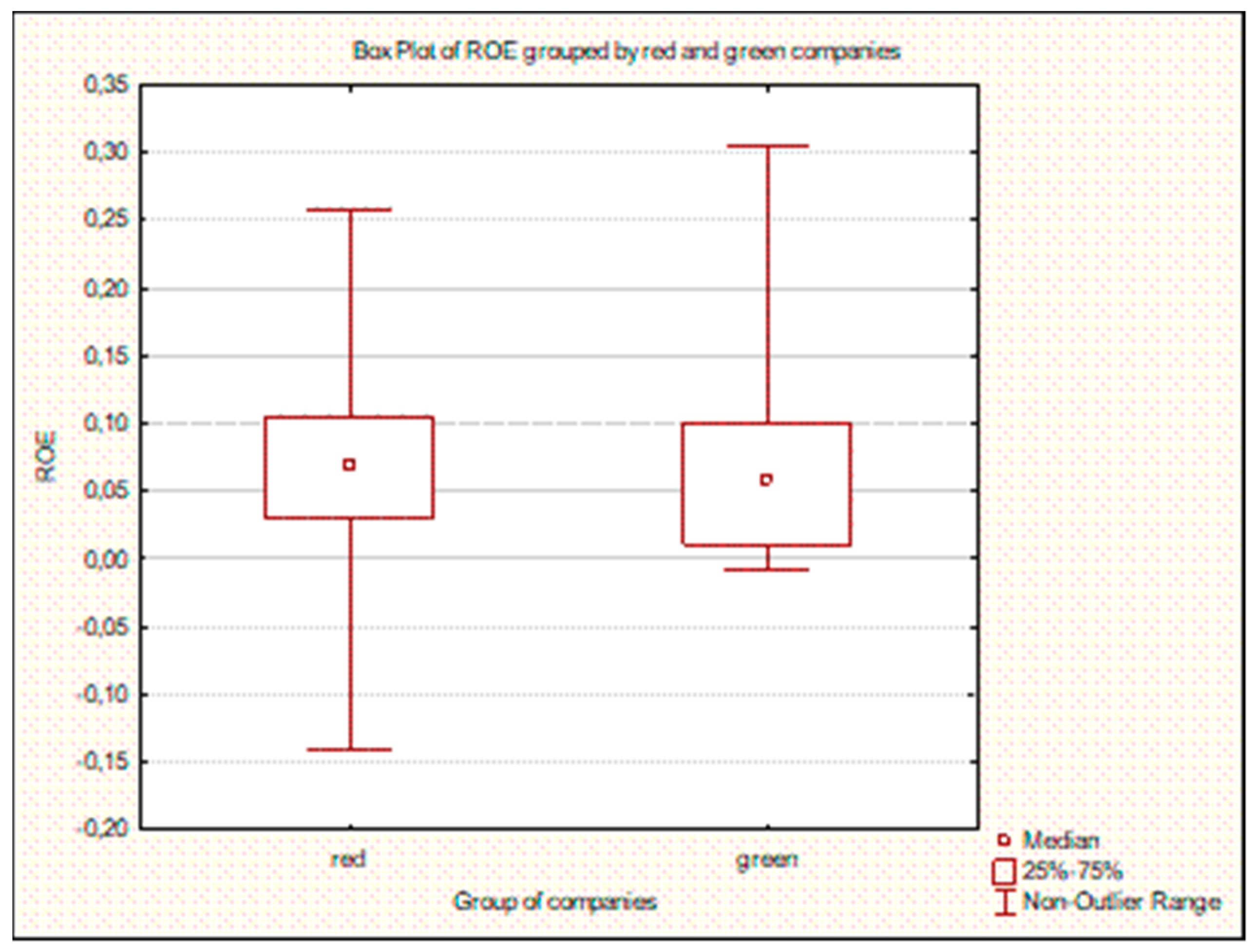
To confirm the accuracy of the resultant classifications, we examined accuracy with various settings for training parameters and apply the 25-fold cross-validation methodology. The calculated risk of cross verification in the output is the risk averaging for 25 test samples. Subsampling DTs are not shown for n-fold cross verification. Only the DT constructed on the full sample is reported. Similarly, only the full sample classification table is reported. Finally, we also investigate whether based upon the results obtained and the analysis of profitability ratios, green companies exhibit superior performance relative to the remainder of the sector. We point out the most critical indicators occurring in the tree and we test the statistical significance of differences in the selected indicators between groups of companies using the Student’s t-test.

3. Results

This section is organized as follows. First, data analysis in defined samples is presented. Then, DT results are shown for outcomes of the 25-fold cross-validation. Next, the analysis of selected of critical indicators is given. Finally, the analysis of profitability ratios is introduced. The outcome of research is presented in Table 3, Table 4, Table 5, Table 6, Table 7, Table 8, Table 9, Table 10, Table 11, Table 12, Table 13, Table 14, Table 15, Table 16, Table 17, Table 18, Table 19, Table 20, Table 21, Table 22, Table 23, Table 24, Table 25 and Table 26 and Figure 3, Figure 4 and Figure 5.

3.1. Data Analysis in Defined Samples

We investigate whether the data can be further analyzed and whether the variables are correctly differentiated in the defined samples. Several methods are applied for this purpose. Firstly, basic statistics are calculated for each sample for all variables. These are the minimum value, the maximum value, arithmetic means, standard deviation and variation coefficients. The obtained values exhibit proper characteristics and correctness of data for all analyzed samples in that scope (example calculated values for the database RG_38V for all companies and for green and red ones are presented in Table 3, Table 4 and Table 5). For each variable, the variation coefficient exceeds the recommended critical value (higher than 0.1 or 0.15). We can therefore proceed with our analysis.
An analysis of the reliability of the variables is also undertaken and we set out to determine whether differentiation in our defined is sufficient for further research. For this purpose, we estimate Cronbach’s alpha for the databases and report the results in Table 6. The objective is to eliminate indicators that do not show sufficient differentiation.
The samples with the lowest Cronbach’s alpha are the databases constructed using eight indicators. These are the sample with a large disproportion between red and green records (RG_8V) and the balanced sample (RG_BD_8V). However, both values indicate the viability for further analysis. The remaining four samples exhibit sufficiently high variable differentiation. The largest differentiation occurs in the sample comprising a balanced number of records of red and green companies for all 62 indicators (RG_BD_62V). A slightly lower value is obtained for the database comprising all 62 indicators (RG_62V) but without a balanced number of records for both groups of companies. The remaining two groups (RG_38V, RG_BD_38V) show slightly lower but nevertheless sufficient differentiation. Our Cronbach’s alpha estimates confirm the viability of further analysis for the groups of variables in all samples.

3.2. DT Results for Whole Companies

The first samples include 38 indicators. It comprises 486 companies, of which 402 are red companies and the remaining 84 are green companies. To limit the size of our DTs in the beginning, the minimum number of observations in the parent node is defined as 100 and the child node as 50 The algorithm identifies four independent variables, namely the short-term liabilities to operating expenses ratio (X51), days sales of inventory II ratio (X46), days sales of inventory I ratio (X20) and the debt to assets ratio (X2), to construct the DT. The DT subsequently comprises nine nodes, including five end nodes. Unfortunately, the classification matrix following the application of 25-fold cross-validation indicates that it is not possible to correctly classify companies in relevant groups. The effect of cross-validation for various numbers of companies in parent and child nodes is presented in Table 5. The algorithms identify financial ratios which unambiguously show that a company manufactures RES component or not. Next, we reduced the number of companies in the parent and child node to 50 and then 25, followed by a reduction to 20 and finally to 10. The reduction in the number of companies in the nodes improves classification ability attributable to the algorithms. The effect of cross-validation for a different number of records at parent and child nodes is reported in Table 7.
We note that the short-term liabilities to operating expenses (X51) ratio, is the most important ratio, according to which the first classification in the DT is established. The second one is X46 days sales of inventory II. Cross-validation for the CRT algorithm is at 99.0% for red and 20.2% for green companies respectively and the QUEST algorithm achieves a cross-validation level of 97.5% for red companies and 19.0% for green companies, respectively. According to the QUEST algorithm, the first classifying ratio is the equity to total asset ratio (X10). The QUEST algorithm underperforms the CHAID algorithm, as reported in Table 8.
A further consideration is whether a reduction in the number of indicators coupled with a simultaneous increase in the number of companies in the sample will positively impact the classification capability of DT algorithms. A reduced number of indicators permits the definition of a sample with a higher number of companies. The sample of only eight ratios comprises 2120, of which 479 are green companies.
The classification option for the sample constructed in this way has been checked using all three DT algorithms. The materiality level for division nodes is set at the level of 0.05 permitting a maximum number of 100 iterations and Pearson’s chi-square statistics are applied. DT extension is limited to a maximum of three levels. In application of DTs to the RG_8V sample, cross-validation shows very poor accuracy correctness. All three DT algorithms are applied to 20 companies in the parent node and 10 in the child node (Table 9).
Next, we construct a sample for all indicators which is accompanied by a decrease in the number of companies This sample comprises 62 variables and 305 companies, including 37 records green companies which means 12.13% of all companies in the sample The number of records of parent and child nodes has been reduced to proportions of 20 and 10. We leave DT size unchanged at the third level as no material changes are observed in the other levels. Following the reduction in the number of records in parent and child nodes, the CHAID algorithm produces a correct classification rate of 96.6% for red companies and 29.7% for green companies. Of all DT algorithms, the CHAID algorithm produces the best results whereas the CRT algorithm underperforms classifying 96.6% of red companies and 27.0% of green companies correctly. The QUEST algorithm does not show any classification capability for green companies (see Table 10).
Based upon these results, the question that can be posed is as to whether a reduction in the disproportion between the number of records for green and red companies respectively in the databases will have a material impact on the classification capacity of the algorithm. Consequently, we balance the number of companies in all databases under consideration. The balanced database with the main eight indicators (RG_BD_8V) comprises 963 companies of which 479 constitute green enterprises. The balanced database with 38 indicators (RG_BD_38V) comprises 188 companies, of which 84 are green enterprises. The database with the highest number of indicators (RG_BD_62V)_ comprises only 77 companies, of which 37 are green companies. The results of this classification are presented in Table 13.
Similar to the databases with an unbalanced and balanced number of green and red companies with 38 indicators (RG_38V & RG_BD_38V), the classifying ratio according to which the first division the DT is undertaken is X51. Balancing records in this database brings the expected effect in the form of a material improvement in the DT classification of companies. The number of correctly classified companies now exceeds 50%. The CHAID algorithm produces the most favourable results, with the number of records in the parent and child nodes equalling 20 and 10 and an accurate classification rate of 84.6% for red companies and 67.9% for green enterprises (Table 11).
The remaining three algorithms also show material improvements in classification ability. The CRT algorithm, in contrast to CHAID, yields a more accurate classification rate for green companies with 71.4% of companies classified correctly and 81.7% of red companies classified correctly, somewhat fewer than the CHAID algorithm. The QUEST algorithm underperforms, classifying 74.0% of red companies and 58.3% of green companies correctly. In all three cases, the variable used in the first classification is the short-term liabilities to operating expenses ratio (X51) Results are summarized in Table 12.
In the balanced database comprising eight indicators, the reduction in the maximum number of companies in parent and child DT nodes from approximately 100 to 50 and then from 50 to 25, improves classification accuracy, as evident in Table 13. Although the percentage of correctly classified green companies increases from 57.6% to 63.3%, at the same time, the percentage of correctly classified red companies decreases from 66.1% to 61.6%. However, the resultant DT is now larger, with three levels of depth and as many as 12 nodes. This contrasts with 10 nodes in the unbalanced database.
The three years gross profit to asset ratio (X24) is the first classifying ratio in the DT. For the unbalanced database with eight indicators (RG_8V), revenue growth ratio (X21) is the classification ratio the root. Other DT algorithms also show higher correct classification rates. The best classification accuracy for green companies is attained by the CRT algorithm, which correctly classifies 61.2% of red companies and 70.1% of green companies. The classification matrix for all DT algorithms for the balanced database with eight indicators is presented in Table 14.
The balanced database comprising all 62 indicators (RG_BD_62V) comprises the lowest number of records. It is composed of data for 37 green enterprises and 41 red enterprises, comprising a total of 77 records. The number of records in the parent node is set to 50 and then 20 and in the child node to 25 and 10 respectively. The CHAID algorithm produces the best results (Table 15). It correctly classifies 70.3% of green enterprises and 85.0% of red enterprises. The QUEST algorithm underperforms all other algorithms, failing to correctly classify any green enterprises (Table 16).
Using a balanced number of records for red enterprises and green enterprises in all three databases translates into increased classification accuracy for green enterprises. Concurrently, the classification accuracy decreases somewhat for red enterprises (see Table 17).
Using the balanced database (RG_BD_8V) for eight variables, the percentage of correctly classified green enterprises for the database increases from 4.6% to 63.3% and for 38 variable database, the percentage of correctly classified green enterprises increases from 47.6% to 67.9% when the databased is balanced. For the database of 62 variables, it increases from 29.7% to 70.4%.
An analogous our study of classification using decision trees was also carried out for grouped indicators. As previous studies show that only balanced databases give positive effects for the classification of enterprises into green and red (see Table 17), only these databases were used for the study, divided by groups of indicators (see Table 18).
Databases have been built to analyse the indicators indicated in the groups. The indicators included in the group and the indicators used in research to analyse the RG_BD_62V and RG_BD_38V databases are presented in Table 19.
Two balanced databases, namely the RG_BD_ 38V and RG_BD_62V databases, were used for calculations. The most interesting results are presented. Our studies have shown that the CHAID method exhibits the best classification performance. This method was used in this analysis. For group P indicators—the profitability indicators-cross-validation showed a correct classification rate of 85 percent for red enterprises and 70.3 percent for green enterprises (Table 20). The use of cross-validation for a database with fewer indicators (RG_BD_38V) resulted in 88.5 percent of correctly classification red enterprises and 51.2percent of green enterprises. The result is slightly worse for the database with 62 indicators. However, for the group of E indicators, namely efficiency indicators, the result presents an improvement when using a database with 38 indicators (70.2 percent—red, 73.8 percent—green) compared to a database with 62 indicators (95.0 percent—red but only 35.1 percent—green).
Following the removal of a single outlier, the model fit improves significantly. Data on green enterprises from the RG_38V database were used to build a linear regression model. The model was built using the stepwise method. Initially, all 38 variables constituting the examined database were introduced into the model (see Table 3). The least squares method was used to fit a regression through a set of observations. The level of significance for retaining a variable was set at 0.05 and at 0.1 for deletion. The dependent variable is X56 (net profit/equity). Following this variable selection procedure, a model comprising 10 predictors was obtained. This model has the highest value of the coefficient of determination R-squared ( R 2 = 0.990 , R 2 c o r r e c t e d = 0.988 ). The representative equation is as follows:
y =     0.126 + 1.006 × X 31 0.356 × X 48 + 0.262 × X 41 0.00002 × X 60 + 1.49 × X 47 0.088 × X 57 1.310 × X 22 0.025 × X 34 + 0.167 × X 37 + 0.022 × X 51 .
All coefficients are statistically significant (Table 21) and the model exhibits the desired statistical significance (Table 22).
Endogeneity regarding correlated-omitted-variables bias for the built regression model has been tested. For this purpose, the impact threshold for a confounding variable (ITCV) test was used [48,49]. An impact statistic were calculated (ITCV) indicating the minimum impact of a confounding variable that would be needed to render the coefficient statistically insignificant. According to the received value of ITCV, alpha = 0.05, an omitted variable would have to be correlated at 0.983 with the outcome and at 0.983 with the predictor of interest (conditioning on observed covariates) to invalidate an inference based on a threshold of 0.23 for statistical significance. Correspondingly the impact of an omitted variable must be 0.966 (0.983 × 0.983) to invalidate an inference.

3.3. Case Study for Data only for Chinese Companies

Basic research was carried out for 2345 enterprises from various countries, in particular for Asian countries (over 93%). All data was for 2017. First, estimations for all companies were made and they became the basis for calculations for which only Chinese companies were selected from the database. The data constitutes almost 75% of the entire database. The database configured in this way was used to build two databases for enterprises in China, one with 8 indicators and the other with 38 indicators. A database of financial results of Chinese enterprises was used for the calculations. Initially, the database comprised 1742 observations in total (almost 75% of the previous database with data from several different countries), of which 1267 were red enterprises and 475—green enterprises. Because previous studies have shown that the decision tree algorithm works best on databases with an equal number of green and red enterprises, the database has been balanced. Finally, due to lack of data, two databases for Chinese enterprises with different numbers of indicators (8 and 38) and balanced but also different numbers of observations were built (Table 23).
Calculations have been made for these two balanced databases. The result of the classification is similar to the results for the database in which enterprises were mixed from several countries (Table 24). This is due to the fact that data for Chinese companies constitutes the majority in the analysed database (almost 75%). The first division variables were X21 and X8 respectively

3.4. Analysis of Critical Indicators

The use of DTs makes it possible to identify important indicators that distinguish companies within the sector. The list of our classifying ratios is presented in Table 25. Five ratios represent different groups of ratios, relating to liquidity, turnover, one from our initial analysis and profitability.
We identify the short-term liabilities to operating expenses ratio (X51) as the most important ratio for classification. The second most important ratio is the revenue growth ratio (X21). On the other hand, the last one is the size of working capital ratio. This ratio is also used in bankruptcy prediction models for manufacturing companies and its inclusion is motivated by Altman’s (1968) model [32]. In Table 26, the differences between the estimated values of financial ratios associated with green and red companies are tested.
Aside from the revenue growth ratio (for two databases, RG_62V and RG_BD_62V), these results confirm that the differences in ratios are statistically significant. This confirms that these ratios are important for classifying companies belonging to the semiconductor and solid state device manufacturing sector. Moreover, green companies that produce components for renewable energy sources (RES) are characterized by lower financial ratios except the payables to operating expenses ratio, which indicate generally higher levels of debt.

3.5. Analysis of Profitability Ratios

The analysis of selected indicators shows that only one profitability indicator has been identified as critical. Therefore, key indicators from the investor and manager’s point of analyzed in this subsection are the namely the return on assets (ROA), the return on sales (ROS) and the return on equity (ROE) ratios. It is worth adding that the selected profitability ratios were calculated for China given its representativity in the sample. Three-quarters of the sample comprises companies operate in China. Figure 3, Figure 4 and Figure 5 also confirm that green companies are described by lower profitability ratios, which are the ROA (X7), ROS (X19) and ROE (X31) ratios.

4. Conclusions

Our study investigates whether investing in the solar technology manufacturers’ components is a lucrative business by analysing the semiconductor and related device manufacturing sector. To do so, we apply a novel approach for the sector, namely DTs. We consider 62 financial ratios and our initial database comprises 2345 companies, mostly operating in China. The companies in the sector are classified into two groups, green companies which are those for which production is related to renewable energy and red companies which are those for which production is not related to renewable energy. We define six samples, both balanced and unbalanced samples and comprising large and small samples of companies and 25-fold cross-validation, which does not significantly improve the results. The literature reports on RES companies, with most of the existing literature related to power plants [21,22], electric utilities [24] or energy companies [30]. Our results are similar to other studies of RES companies. On the basis of certain financial ratios, we find that green companies underperform red companies [21,22]. Our contribution lies in addressing the lack of studies that assess the relative financial performance of companies that provide equipment needed for renewable energy production. Moreover, we apply DTs for the purposes of identifying classifying ratios.
The decision tree based analysis identifies the most important indicators for evaluating enterprises, especially for those operating in China. This provides a broader overview of the financial standing of groups of companies to managers and investors. Our results indicate that investing in companies that manufacture RES components may not be a lucrative business. For managers, this is important information that indicates that RES companies are not profitable or as financially sound relative to companies in the general semiconductor and solid state device manufacturing sector. For investors potentially interested in investing in RES associated companies, our findings demonstrate a need for caution. This should be viewed within the context of achieving RES targets in total energy production. Given government targets for renewable energy, the demand for components for renewable energy production will increase. However, it remains to be seen whether this increase in demand will accompany profits.
The topic chosen by us for analysis is difficult and multi-threaded but it is worth making a foundation for further research. Our research provides a solid basis for further exploration of this data. With this foundation in place, we can continue research in the directions indicated by the reviewer. The authors are aware that all factors, both fundamental and economic, may impact the profitability of doing business.
Our analysis, however, focuses on financial ratios and is a good basis for further research. Specifically, we focus on companies within the semiconductor and related device manufacturing sector. The purpose of our work is not to compare which industry is more profitable for the investor but to determine whether selected financial indicators will indicate differences between enterprises related to the production of semi-finished products for renewable energy production and conventional energy.
Given the importance of renewable energy sources for investors, information on the profitability of not only these enterprises themselves but also enterprises in the entire production chain is crucial. Our research is significant and fills the gap in the analysed area regarding the analysis of financial indicators for enterprises from the semiconductor and related device manufacturing sector.
We recognize some of the limitations of our study. First, the research period only encompasses 2017. This may influence results. We are faced with this limitation owing to missing data for the years 2008-2016. Second, three-quarters of analysed enterprises in our sample are from China. Third, we only rely upon financial ratios in our study. Finally, we limit ourselves to applying only DTs in this study. Other approaches, such as neural network (NN) can also be used for classification purposes.

Supplementary Materials

The following are available online at https://www.mdpi.com/1996-1073/13/2/499/s1, File consists of Tables S1–S6. Table S1. RG_8V; 8 variables, unbalanced number of companies, N = 2120. Table S2. RG_BD_8V; 8 variables, balanced number of companies, N = 963. Table S3. RG_38V; 38 variables, unbalanced number of companies, N = 486. Table S4. RG_BD_38V, 38 variables, balanced number of companies, N = 188. Table S5. RG_62V, 62 variables, unbalanced number of companies, N = 305. Table S6. RG_BD_62V; 62 variables, balanced number of companies, N = 77. ID concerns red enterprises (0) and green enterprises (1); colour concerns red enterprises (C) and green enterprises (Z).

Author Contributions

Conceptualization, S.K.T., A.S.-S.; and J.J.S.; methodology, S.K.T., A.S.-S.; software, S.K.T., A.S.-S.; validation, S.K.T., A.S.-S.; formal analysis, S.K.T., A.S.-S.; investigation, S.K.T., A.S.-S.; resources, S.K.T., A.S.-S; data curation, S.K.T.; writing—original draft preparation, S.K.T., A.S.-S., J.J.S.; writing—reviewing and editing, S.K.T., J.J.S.; visualization, S.K.T.; supervision, S.K.T.; project administration, S.K.T.; funding acquisition, S.K.T. All authors have read and agreed to the published version of the manuscript.

Funding

This research was funded by Wrocław University of Science and Technology, financed from statutory funds, project No. 0402/0135/18.

Conflicts of Interest

The authors declare no conflict of interest.

References

  1. The International Energy Agency. Available online: https://www.iea.org/statistics (accessed on 30 October 2019).
  2. Independent Evaluation Group. CHINA Renewable Energy Scale-Up Program: Phase One, Report No. 117156. 2017. Available online: https://ieg.worldbankgroup.org/sites/default/files/Data/ppar-chinarenewableenergy-10302017.pdf (accessed on 22 December 2019).
  3. National Institute of Transforming India. Report of Expert Group on 175 GW RE by 2022. 2015. Available online: https://niti.gov.in/writereaddata/files/175-GW-Renewable-Energy.pdf (accessed on 22 December 2019).
  4. The International Energy Agency. Available online: https://www.iea.org/policiesandmeasures/renewableenergy (accessed on 30 October 2019).
  5. The International Energy Agency. Available online: https://www.iea.org/policiesandmeasures/pams/china (accessed on 30 October 2019).
  6. Sinha, A. Here Are India’s INDC Objectives and How Much It Will Cost. Available online: https://indianexpress.com/article/india/india-news-india/here-are-indias-indc-objectives-and-how-much-it-will-cost/ (accessed on 30 October 2019).
  7. Hongzhan, S.; Qiang, Z.; Yibo, W.; Qiang, Y.; Jun, S. China’s solar photovoltaic industry development: The status quo, problems and approaches. Appl. Energy 2014, 118, 221–230. [Google Scholar]
  8. Pablo-Romero, M.P. Solar Energy: Incentives to Promote PV in EU27. AIMS Energy 2013, 1, 28–47. [Google Scholar] [CrossRef] [Green Version]
  9. Solangi, K.H.; Islam, M.R.; Saidur, R.; Rahim Fayaz, H. A review on global energy policy. Renew. Sustain. Energy Rev. 2011, 15, 2149–2163. [Google Scholar] [CrossRef]
  10. Sachu, B.K. A study on global solar PV energy developments and policies with a special focus on the top ten solar PV power producing countries. Renew. Sustain. Energy Rev. 2015, 43, 621–634. [Google Scholar]
  11. Trück, S.; Weron, R. Convenience yields and risk premiums in the EU-ETS—Evidence from the Kyoto commitment period. J. Futures Mark. 2016, 36, 587–611. [Google Scholar] [CrossRef] [Green Version]
  12. Bohl, M.T.; Kaufmann, P.; Stephan, P.M. From hero to zero: Evidence of performance reversal and speculative bubbles in German renewable energy stocks. Energy Econ. 2013, 37, 40–51. [Google Scholar] [CrossRef] [Green Version]
  13. Henriques, I.; Sadorsky, P. Oil prices and the stock prices of alternative energy companies. Energy Econ. 2008, 30, 998–1010. [Google Scholar] [CrossRef]
  14. Inchauspe, J.; Ripple, R.D.; Truck, S. The dynamics of returns on renewable energy companies: A state-space approach. Energy Econ. 2015, 48, 325–335. [Google Scholar] [CrossRef]
  15. Kumar, S.; Managi, S.; Matsuda, A. Stock prices of clean energy firms, oil and carbon markets: A vector autoregressive analysis. Energy Econ. 2012, 34, 215–226. [Google Scholar] [CrossRef]
  16. Managi, S.; Okimoto, T. Does the price of oil interact with clean energy prices in the stock market? Jpn. World Econ. 2013, 27, 1–9. [Google Scholar] [CrossRef] [Green Version]
  17. Maryniak, P.; Trück, S.; Weron, R. Carbon pricing and electricity markets—The case of the Australian Clean Energy Bill. Energy Econ. 2019, 79, 45–58. [Google Scholar] [CrossRef]
  18. Capece, G.; Cricelli, L.; Di Pillo, F.; Levialdi, N. A cluster analysis study based on profitability and financial indicators in the Italian gas retail market. Energy Policy 2010, 38, 3394–3402. [Google Scholar] [CrossRef]
  19. Capece, G.; Cricelli, L.; Di Pillo, F.; Levialdi, N. New regulatory policies in Italy: Impact on financial results, on liquidity and profitability of natural gas retail companies. Util. Policy 2012, 23, 90–98. [Google Scholar] [CrossRef]
  20. Halkos, G.E.; Tzeremes, N.G. Analyzing the Greek renewable energy sector: A Data Envelopment Analysis approach. Renew. Sustain. Energy Rev. 2012, 16, 2884–2893. [Google Scholar] [CrossRef]
  21. Paun, D. Sustainability and financial performance of companies in the energy sector in Romania. Sustainability 2017, 9, 1722. [Google Scholar] [CrossRef] [Green Version]
  22. Tomczak, S.K. Comparison of the Financial Standing of Companies Generating Electricity from Renewable Sources and Fossil Fuels: A New Hybrid Approach. Energies 2019, 12, 3856. [Google Scholar] [CrossRef] [Green Version]
  23. Clarkson, P.M.; Li, Y.; Richardson, G.D.; Vasvari, F.P. Does it really pay to be green? Determinants and consequences of proactive environmental strategies. J. Account. Public Policy 2011, 30, 122–144. [Google Scholar] [CrossRef]
  24. Ruggiero, S.; Lehkonen, H. Renewable energy growth and the financial performance of electric utilities: A panel data study. J. Clean. Prod. 2017, 142, 3676–3688. [Google Scholar] [CrossRef] [Green Version]
  25. Sueyoshi, T.; Goto, M. Can environmental investment and expenditure enhance financial performance of US electric utility firms under the Clean Air Act amendment of 1990? Energy Policy 2009, 37, 4819–4826. [Google Scholar] [CrossRef]
  26. Telle, K. “It pays to be green”—A premature conclusion? Environ. Resour. Econ. 2006, 35, 195–220. [Google Scholar] [CrossRef]
  27. Pätäri, S.; Arminen, H.; Tuppura, A.; Jantunen, A. Competitive and responsible? The relationship between corporate social and financial performance in the energy sector. Renew. Sustain. Energy Rev. 2014, 37, 142–154. [Google Scholar]
  28. Arslan-Ayaydin, Ö.; Thewissen, J. The financial reward for environmental performance in the energy sector. Energy Environ. 2016, 27, 389–413. [Google Scholar] [CrossRef]
  29. Sueyoshi, T.; Goto, M. Data envelopment analysis for environmental assessment: Comparison between public and private ownership in petroleum industry. Eur. J. Oper. Res. 2012, 216, 668–678. [Google Scholar] [CrossRef]
  30. Doumpos, M.; Andriosopoulos, K.; Galariotis, E.; Makridou, G.; Zopounidis, C. Corporate failure prediction in the European energy sector: A multicriteria approach and the effect of country characteristics. Eur. J. Oper. Res. 2017, 262, 347–360. [Google Scholar] [CrossRef]
  31. Bobinaite, V. Financial sustainability of wind electricity sectors in the Baltic States. Renew. Sustain. Energy Rev. 2015, 47, 794–815. [Google Scholar] [CrossRef]
  32. Altman, E.I. Financial Ratios, Discriminant Analysis and the Prediction of Corporate Bankruptcy. J. Financ. 1968, 23, 589–609. [Google Scholar] [CrossRef]
  33. Beaver, W.H. Financial Ratios as Predictors of Failure. J. Acc. Res. 1968, 4, 71–111. [Google Scholar] [CrossRef]
  34. Ohlson, J.A. Financial Ratios and the Probabilistic Prediction of Bankruptcy. J. Acc. Res. 1980, 18, 109–131. [Google Scholar] [CrossRef] [Green Version]
  35. Frydman, H.; Altman, E.I.; Kao, D.L. Introducing recursive partitioning for financial classification: The case of financial distress. J. Finance 1985, 40, 269–291. [Google Scholar] [CrossRef]
  36. Koh, H.C.; Kee Low, C. Going concern prediction using data mining techniques. Manag. Audit. J. 2004, 19, 462–476. [Google Scholar]
  37. Li, H.; Sun, J.; Wu, J. Predicting business failure using classification and regression tree: An empirical comparison with popular classical statistical methods and top classification mining methods. Expert Syst. Appl. 2010, 37, 5895–5904. [Google Scholar] [CrossRef]
  38. Gepp, A.; Kumar, K.; Bhattacharya, S. Business failure prediction using decision trees. J. Forecast. 2010, 29, 536–555. [Google Scholar] [CrossRef]
  39. Fedorova, E.; Gilenko, E.; Dovzhenko, S. Bankruptcy prediction for Russian companies: Application of combined classifiers. Expert Syst. Appl. 2013, 40, 7285–7293. [Google Scholar] [CrossRef]
  40. Zięba, M.; Tomczak, S.K.; Tomczak, J.M. Ensemble boosted trees with synthetic features generation in application to bankruptcy prediction. Expert Syst. Appl. 2016, 58, 93–101. [Google Scholar] [CrossRef]
  41. Balcaen, S.; Ooghe, H. 35 years of studies on business failure: An overview of the classic statistical methodologies and their related problems. Br. Acc. Rev. 2006, 38, 63–93. [Google Scholar] [CrossRef]
  42. Kim, S.Y.; Upneja, A. Predicting restaurant financial distress using decision tree and AdaBoosted decision tree models. Econ. Model. 2014, 36, 354–362. [Google Scholar] [CrossRef]
  43. Larose, D.T. Discovering Knowledge in Data; An Introduction to Data Mining; Wiley-Interscience, A John Wiley Sons, Inc. Publication: Hoboken, NJ, USA, 2005. [Google Scholar]
  44. Kass, G.V. An exploratory technique for investigating large quantities of categorical data. J. R. Stat. Soc. Ser. C (Appl. Stat.) 1980, 29, 119–127. [Google Scholar] [CrossRef]
  45. Breiman, L.; Friedman, J.; Olshen, R.; Stone, C. Classification and Regression Trees; Wadsworth Int. Group: Wadsworth, OH, USA, 1984; Volume 237–251, p. 37. [Google Scholar]
  46. Loh, W.Y.; Shih, Y.S. Split selection methods for classification trees. Statistica Sinica 1997, 7, 815–840. [Google Scholar]
  47. IBM Knowledge Center. 2019. Available online: https://www.ibm.com/support/knowledgecenter/SSLVMB_subs/statistics_casestudies_project_ddita/spss/tutorials/tree_missing_crt_results.html (accessed on 15 October 2019).
  48. Frank, K. Impact of a Confounding Variable on the Inference of a Regression Coefficient. Sociol. Methods Res. 2000, 29, 147–194. [Google Scholar] [CrossRef]
  49. He, G.; Bai, L.; Ren, H.M. Analyst coverage and future stock price crash risk. J. Appl. Acc. Res. 2019, 20, 63–77. [Google Scholar] [CrossRef] [Green Version]
Figure 1. Global electricity generation from renewable sources, 1990–2017. Data source: [1].
Energies 13 00499 g001
Figure 2. Electricity generation from renewable sources; share in the overall energy production for selected countries, 2010–2017 (in %). Data source—[1,4,5,6]. Target for Turkey, People’s Republic of China, India is for 2030, target for Chinese Taipei is for 2025 and target for Thailand is for 2036; * means the percentage of non-fossil energy in total electric power generation.
Energies 13 00499 g002
Figure 3. Return on assets (ROA) values for red and green companies.
Energies 13 00499 g003
Figure 4. Return on sales (ROS) values for red and green companies.
Energies 13 00499 g004
Figure 5. Return on equity (ROE) values for red and green companies.
Energies 13 00499 g005
Table 1. List of ratios considered.
NoDefinitionGroupNoDefinitionGroup
1net profit/total assetsP32(current liabilities × 365)/cost of products soldT
2total liabilities/total assetsS33operating expenses/short-term liabilitiesS
3working capital/total assetsL34operating expenses/total liabilitiesS
4current assets/short-term liabilitiesL35profit on sales/total assetsP
5[(cash + short-term securities + receivables − short-term liabilities)
/(operating expenses − depreciation)] ∗ 365
L36(current assets − inventories)/long-term liabilitiesL
6retained earnings/total assetsP37constant capital/total assets O
7EBIT/total assetsP38profit on sales/salesP
8book value of equity/total liabilitiesS39(current assets − inventory − receivables)/short-term liabilitiesL
9sales/total assetsE40total liabilities/((profit on operating activities + depreciation) ×
(12/365))
S
10equity/total assetsS41profit on operating activities/salesP
11(gross profit + extraordinary items + financial expenses)/total
assets
P42rotation receivables + inventory turnover in daysL
12gross profit/short-term liabilitiesS43(receivables × 365)/salesE
13(gross profit + depreciation)/salesP44net profit/inventoryE
14EBIT/total costsS45(current assets − inventory)/short-term liabilitiesL
15(total liabilities ∗ 365)/(gross profit + depreciation)S46(inventory × 365)/cost of goods soldE
16(gross profit + depreciation)/total liabilitiesS47EBITDA/total assetsP
17total assets/total liabilitiesS48EBITDA/salesP
18gross profit/total assetsP49current assets/total liabilitiesS
19EBIT/salesP50short-term liabilities/total assetsS
20(inventory ∗ 365)/salesE51short-term liabilities/operating expensesS
21sales (n)/sales (n − 1)O52equity/fixed assetsO
22profit on operating activities/total assetsP53constant capital/fixed assetsO
23net profit/salesP54working capitalL
24gross profit (in 3 years)/total assetsP55(sales − cost of products sold)/salesP
25(equity − share capital)/total assetsS56net profit/equityP
26(net profit + depreciation)/total liabilitiesS57long-term liabilities/equityS
27profit on operating activities/financial expensesE58sales/inventoryE
28working capital/fixed assetsL59sales/receivablesE
29logarithm of total assetsO60(short-term liabilities × 365)/salesE
30(total liabilities − cash)/salesO61sales/short-term liabilitiesE
31EBIT/equityP62sales/fixed assetsE
P—represents profitability ratios, L—represents liquidity ratios, S—represents solvency ratios, E—represents efficiency ratios and O—represents other ratios.
Table 2. Overview of samples used and the number of financial ratios for each sample.
Sample NameNumber of RatiosNumber of CompaniesNumber of Red CompaniesNumber of Green Companies
RG_8V
(X1, X7, X9, X19, X21, X23, X24 i X29)
821201641479
RG_38V
(see Table 3)
3848640284
RG_62V
(see Table 1)
6230526837
RG_BD_8V8963484479
RG_BD_38V3818810484
RG_BD_62V62774137
Table 3. Statistical characteristics for all quantitative variables across samples.
RatioMinMaxAverageStandard DeviationCoefficient of Variation
X20.013.430.420.310.73
X3−3.270.860.240.361.47
X40.04649.633.023.831.27
X8−0.7199.243.246.221.92
X10−2.430.990.580.310.53
X12−6.005.350.120.786.34
X170.29100.244.246.221.47
X18−4.043.090.110.554.91
X20−7417.70965.7754.21346.956.40
X22−0.530.330.0250.103.82
X25−6.620.940.250.572.31
X28−3.8881.231.795.052.83
X30−626.60242.700.4032.4480.22
X31−3.261.320.0270.3312.08
X33−0.00328.103.022.730.90
X34−0.00328.102.422.481.03
X37−2.430.990.670.280.42
X390.00342.741.773.301.86
X41−7.2916.070.0080.89119.71
X42−54,297.551285.7682.192476.8630.14
X43−46,879.851273.2527.982136.8276.38
X44−213.9040.10−0.51110.88−21.26
X450.02748.862.293.651.59
X46−11.70968.9772.1073.911.03
X47−0.560.370.0630.0961.53
X48−5.753.790.0740.496.65
X490.04626.742.392.931.23
X500.0093.430.330.280.85
X51−358.6791.380.1716.88101.14
X52−3.2278.632.534.921.94
X53−2.8882.232.795.051.81
X54−1,884,438.6416,728,068.12155,327.351,045,613.846.73
X56−3.632.13−0.0010.35−304.85
X57−0.863.840.230.441.96
X59−0.008275.806.2513.722.20
X60−122,108.8596,597.68418.968107.6919.35
X61−0.00328.733.162.810.89
X62−0.009322.384.9217.933.65
RG_38V, 38 variables, unbalanced number of companies, N = 486.
Table 4. Statistical characteristics for all quantitative variables across samples—green companies.
RatioMinMaxAverageStandard DeviationCoefficient of Variation
X20.093.430.610.500.82
X3−3.270.820.030.5618.22
X40.057.571.661.450.88
X8−0.7110.631.391.771.27
X10−2.430.910.390.501.29
X12−3.342.33−0.020.58−31.56
X170.2911.632.391.770.74
X18−2.401.090.000.3779.84
X20−7417.70476.18−12.47822.06−65.92
X22−0.530.240.000.10−104.93
X25−2.620.780.060.6110.07
X28−3.8819.930.823.063.72
X30−626.6040.70−5.3268.84−12.94
X31−3.251.32−0.030.52−16.98
X330.058.291.701.500.88
X340.026.571.281.210.94
X37−2.430.940.520.470.91
X390.014.700.680.841.24
X41−7.2916.070.032.0057.30
X42−54,297.551285.76−368.805959.94−16.16
X43−46,879.851273.25−356.335142.79−14.43
X44−213.9018.12−3.2323.79−7.35
X450.035.770.991.051.06
X461.23530.3982.5599.721.21
X47−0.520.310.030.103.30
X48−5.753.790.000.94−193.69
X490.056.261.241.110.89
X500.063.430.480.471.00
X510.1222.201.543.071.99
X52−3.2220.581.493.032.04
X53−2.8820.931.823.061.68
X54−1,884,438.641,515,112.9970,859.24392,833.745.54
X56−3.302.14−0.060.59−9.46
X57−0.862.580.360.561.55
X59−0.01275.807.3129.904.09
X60−122,108.8514,857.05−698.1913,558.95−19.42
X610.008.751.741.480.85
X62−0.0114.921.982.781.41
Green_38V, 38 variables, green companies, unbalanced number of companies, N = 84.
Table 5. Statistical characteristics for all quantitative variables across samples—red companies.
RatioMinMaxAverageStandard DeviationCoefficient of Variation
X20.011.950.380.230.60
X3−1.510.860.290.280.97
X40.1649.633.314.101.24
X8−0.4999.243.636.731.85
X10−0.950.990.620.230.37
X12−6.005.350.150.815.32
X170.51100.244.636.731.45
X18−4.043.090.130.584.30
X200.00965.7768.1567.740.99
X22−0.300.330.030.093.06
X25−6.620.940.290.551.94
X28−2.6781.231.995.352.69
X30−4.66242.701.6016.8510.53
X31−3.260.540.040.266.79
X330.0028.103.302.850.86
X340.0028.102.662.610.98
X37−0.950.990.700.210.29
X390.0042.742.003.561.78
X41−3.961.740.000.37213.50
X428.631044.46176.43127.430.72
X430.001022.05108.28103.570.96
X44−41.7240.100.064.9185.60
X450.0648.862.563.941.54
X46−11.70968.9769.9267.240.96
X47−0.280.370.070.091.35
X48−3.501.620.090.323.58
X490.0726.742.633.131.19
X500.011.950.300.210.69
X51−358.6791.38−0.1218.50−153.02
X52−1.6778.632.755.201.89
X53−1.6782.232.995.351.79
X54−1,042,686.2216,728,068.12172,977.401,135,157.446.56
X56−3.630.800.010.2723.77
X57−0.013.840.200.412.07
X590.0071.296.036.501.08
X6012.7196,597.68652.396413.729.83
X610.0028.733.452.930.85
X620.00322.385.5319.623.55
Red_38V, 38 variables, red companies, unbalanced number of companies, N = 402.
Table 6. Cronbach’s alpha across samples.
Database NameCronbach’s Alpha
RG_8V0.467
RG_38V0.796
RG_62V0.820
RG_BD_8V0.380
RG_BD_38V0.797
RG_BD_62V0.857
Table 7. Cross-validation classification matrix for 25-fold cross-validation for sample of RG_38V and decision tree (DT) algorithm: CHAID.
The Number of Records in the Parent and Child Nodes: 100 and 50
Observedpredicted
CZpercentage correct
C4020100.0%
Z8400.0%
total percentage100.0%0.0%82.7%
The Number of Records in the Parent and Child Nodes: 50 and 25
Observedpredicted
CZpercentage correct
C3762693.5%
Z513339.3%
total percentage87.9%12.2%84.2%
The Number of Records in the Parent and Child Nodes: 20 and 10
Observedpredicted
CZpercentage correct
C3663691.0%
Z444047.6%
total percentage84.4%15.6%83.5%
Table 8. Cross-validation classification matrix for the RG_38V sample for the three DT algorithms.
AlgorithmRedGreenFirst Division Variable
CHAID91.0%47.6%X51
CRT99.0%20.2%X51
QUEST97.5%19.0%X10
Sample with dependant variable as colour (C—red enterprises, Z—green enterprises). Number of records in parent and child nodes: 20 and 10.
Table 9. Cross-validation classification matrix for the database RG_8V.
AlgorithmRedGreenFirst Division Variable
CHAID99.1%4.6% X21
CRT97.9%13.6%X21
QUEST100.0%0.0%X21
Three algorithms for DTs with, dependent variable; colour (C—red enterprises, Z—green enterprises), number of records in parent and child nodes: 20 and 10.
Table 10. Cross-validation classification matrix for database RG_62V database.
AlgorithmRedGreenFirst Division Variable
CHAID96.6%29.7%X5
CRT96.6%27.0%X50
QUEST100.0%0.0%No variable
Three algorithms, CHAID, CRT and QUEST algorithms applied for DT construction. The dependant variables are green and red companies. The number of records in parent and child nodes is set to 20 and 10 respectively.
Table 11. Cross-validation classification matrix for the RG_BD_38V sample using the CHAID algorithm.
The Number of Records in the Parent and Child Nodes: 100 and 50
Observedpredicted
CZpercentage correct
C812377.9%
Z325261.9%
total percentage60.1%39.9%70.7%
The Number of Records in the Parent and Child Nodes: 50 and 25
Observedpredicted
CZpercentage correct
C97793.3%
Z463845.2%
total percentage76.1%23.9%71.8%
The Number of Records in the Parent and Child Nodes: 20 and 10
Observedpredicted
CZpercentage correct
C881684.6%
Z275767.9%
total percentage61.2%38.8%77.1%
Table 12. Cross-validation classification matrix for the RG_BD_38V sample.
AlgorithmRedGreenFirst Division Variable
CHAID84.6%67.9%X51
CRT81.7%71.4%X51
QUEST74.0%58.3%X51
Three algorithms of tree building, dependant variable: colour (C—red enterprises, Z—green enterprises), number of records in parent and child nodes: 20 and 10.
Table 13. Cross-validation classification matrix for the RG_BD_8V sample, tree-building algorithm: CHAID.
The Number of Records in the Parent and Child Nodes: 100 and 50
Observedpredicted
CZpercentage correct
C32016466.1%
Z20327657.6%
total percentage54.3%45.7%61.9%
The Number of Records in the Parent and Child Nodes: 50 and 25
Observedpredicted
CZpercentage correct
C29818661.6%
Z17630363.3%
total percentage49.2%50.8%62.4%
The Number of Records in the Parent and Child Nodes: 20 and 10
Observedpredicted
CZpercentage correct
C29818661.6%
Z17630363.3%
total percentage49.2%50.8%62.4%
Table 14. Cross-validation classification matrix for the database RG_BD_8V.
AlgorithmRedGreenFirst Division Variable
CHAID61.6%63.3%X24
CRT61.2%70.1%X24
QUEST60.1%59.9%X29
Four algorithms of tree building, dependant variable: colour (C—red enterprises, Z—green enterprises), number of records in parent and child nodes: 20 and 10.
Table 15. Cross-validation classification matrix for the RG_BD_62V database, tree-building algorithm: CHAID.
The Number of Records in the Parent and Child Nodes: 50 and 25
Observedpredicted
CZpercentage correct
C271367.5%
Z122567.6%
total percentage50.6%49.4%67.5%
The Number of Records in the Parent and Child Nodes: 20 and 10
Observedpredicted
CZpercentage correct
C34685.0%
Z112670.3%
total percentage58.4%41.6%77.9%
Table 16. Cross-validation classification matrix for the RG_BD_62V database.
AlgorithmRedGreenFirst Division Variable
CHAID85.0%70.3%X3
CRT75.0%67.6%X6
QUEST100.0%0.0%Variables not considered
Three algorithms of tree building, dependant variable: colour (C—red enterprises, Z—green enterprises), number of records in parent and child nodes: 20 and 10.
Table 17. Percentage of correctly classified enterprises based upon cross-validation for all analysed samples.
The Number of Records in the Parent and Child Nodes: 100 and 50
RG_BD_8VRG_8VRG_BD_38VRG_38VRG_BD_62VRG_62V
C66.1%100.0%77.9%100.0%------100.0%
Z57.6%0.0%61.9%0.0%------0.0%
The Number of Records in the Parent and Child Nodes: 50 and 25
RG_BD_8VRG_8VRG_BD_38VRG_38VRG_BD_62VRG_62V
C61.6%99.1%93.3%93.5%67.5%100.0%
Z63.3%4.6%45.2%39.3%67.6%0.0%
The Number of Records in the Parent and Child Nodes: 20 and 10
RG_BD_VRG_8VRG_BD_38VRG_38VRG_BD_62VRG_62V
C61.6%99.1%84.6%91.0%85.0%96.6%
Z63.3%4.6%67.9%47.6%70.4%29.7%
Tree-building algorithm: CHAID, dependant variable: colour (C, Z).
Table 18. Overview of samples used and the number of financial ratios for each sample.
Sample NameNumber of Variable Groups and Indicators
RG_BD_8V 8Group P: X1, X7, X19, X23, X24
RG_BD_38V38Group D: X2, X8, X10, X12, X17, X25, X33, X34, X49, X50, X51, X57;
Group L: X3, X4, X28, X39, X45, X54;
Group T: X20, X42, X43, X44, X46, X59, X61, X62
RG_BD_62V62All indicator groups, all indicators
Table 19. Indicators included in the group and those used in the analysis of the RG_BD_62V and RG_BD_38V databases.
GroupRG_BD_62V
P: X1, X6, X7, X11, X13, X18, X19, X22, X23, X24, X31, X35, X38, X41, X47, X48, X55, X56,
S: X2, X8, X10, X12, X14, X15, X16, X17, X25, X26, X33, X34, X40, X49, X50, X51, X57,
L: X3, X4, X5, X28, X36, X39, X45, X54,
E: X9, X20, X32, X42, X43, X44, X46, X58, X59, X60, X61, X62,
O: X21, X27, X29, X30, X37, X52, X53,
GroupRG_BD_38V
S: X2, X8, X10, X12, X17, X25, X33, X34, X40, X49, X50, X51, X57,
L: X3, X4, X28, X39, X45, X54,
E: X20, X42, X43, X44, X46, X59, X61, X62,
Table 20. Cross-validation classification matrix for the RG_BD_38V sample and the RG_BD_62V sample for the DT algorithm for indicator groups.
Groups of IndicatorsRedGreenFirst Division Variable
RG_BD_62V
Group P85.0%70.3%X55
Group S85..0%45.9%X40
Group L95.0%35.1%X3
Group E100.0%0.0%No variable is included
Group O95.0%35.1%X52
RG_BD_38V
Group S88.5%51.2%X33
Group L75.0558.3%X4
Group E70.2%73.8%X46
Sample with dependant variable as colour (C—red enterprises, Z—green enterprises).
Table 21. Statistical significance of indicators.
ModelVariableSignificance
(Constant) 0.002
X31EBIT/equity0.000
X48EBITDA/sales0.000
X41profit on operating activities/sales0.000
X60sales0.000
X47EBITDA/total assets0.000
X57long-term liabilities/equity0.000
X22profit on operating activities/total assets0.018
X34operating expenses/total liabilities0.001
X37constant capital/total assets0.000
X51short-term liabilities/operating expenses0.015
Table 22. Statistical significance of the regression model.
Anova a
ModelSum of SquaresdfMean SquareFSignificance
Regression28.123102.812694.8390.000
Rest0.295730.004
Altogether28.41983
a Dependent variable: X56. Predictors: (Constant), X31, X48, X41, X60, X47, X57, X22, X34, X37, X51.
Table 23. Overview of samples used and the number of financial ratios for each sample.
Sample NameNumber of Ratios Number of CompaniesNumber of Red CompaniesNumber of Green Companies
China_RG_BD_8V
(X1, X7, X9, X19, X21, X23, X24 i X29)
8843422421
China_RG_BD_38V
(see Table 3)
381158332
Table 24. Percentage of correctly classified enterprises based upon cross-validation for analysed samples.
China_RG_BD_8VRG_BD_8VChina_RG_BD_38VRG_BD_38V
C69.2%61.6%72.7%84.6%
Z55.8%63.3%71.9%67.9%
Tree-building algorithm: CHAID, dependant variable: colour (C, Z).
Table 25. Summary of the most important indicators.
RatioDefinitionClassification ThresholdGroup
X51short-term liabilities/operating expenses≤0.84389330637; >0.84389330637
≤0.69232544490; >0.69232544490
Efficiency
X21sales (n)/sales (n − 1)≤0.92510251238; >0.92510251238 Other
X5[(cash + short-term securities + receivables − short-term liabilities)/(operating expenses − depreciation)] × 365≤−154.4882205507; >−154.4882205507Liquidity
X24gross profit (in 3 years)/total assets≤0.101199752312; >0.101199752312Profitability
X3working capital/total assets≤–0.04734495587; >−0.04734495587Liquidity
Table 26. The Student’s t-test results for each sample for most important ratios.
RatioREDGREENt-Valuedfp
RG_8V
X211.070.994.2620170.000021 ***
X240.110.064.9019360.000001 ***
RG_BD_8V
X211.060.992.419080.016344 **
X240.110.064.908850.000001 ***
RG_38V
X30.300.135.534750.000000 ***
X510.430.65−6.044340.000000 ***
RG_BD_38V
X30.270.124.131810.000055 ***
X510.520.81−4.721740.000005 ***
RG_62V
X30.300.172.932570.003719 ***
X547.28−10.982.302570.022226 **
X211.071.021.222570.225125 *
X240.06−0.062.542570.011714 **
X510.390.49−2.282570.023180 **
RG_BD_62V
X30.270.142.30660.024833 **
X540.51−37.982.19660.032349 **
X211.051.050.11660.912253 *
X240.098−0.052.49660.015349 **
X510.410.54−2.18660.033077 *
* indicates statistical significance at 10%, ** indicates statistical significance at 5% and *** indicates statistical significance at 1%.

