A Converter with Automatic Stage Transition Control for Inductive Power Transfer

Abstract

An automatic stage transition converter for an inductive power transfer system is presented in this paper. An effective control strategy with two working stages of independent energy injection stage and free resonance stage is employed in the proposed converter. With the automatic stage transition strategy, when the frequency of the resonance network changes, the ending time of the free resonance stage is automatically determined. At the same time, the phase angle of the free resonance stage is automatically set as half a resonant cycle. As the stage transition is not triggered by the switches, the switch motion can be executed in advance of the transition moments. Time margins are offered for every switch in the converter, which make the switching moments of the switches flexible and the control simple. Another feature of this converter is that during the energy injection stage, the energy is injected into the inductor independently. Therefore, the input power can be easily regulated by adjusting the energy injection time. A prototype for the converter and the inductive power transfer system was implemented experimentally. From the experimental results, the automatic stage transition and power regulation capability of the proposed converter are verified. The switches all operated at the soft switch condition. When the energy injection time was adjusted from 10 μs to 25 μs, the output power changed from 143 W to 740 W.

1. Introduction

Wireless power transfer (WPT) technology is a promising approach to deliver power without physical contact and has been widely employed for many applications [1,2,3,4,5]. In the past decade, as a popular technology of WPT, inductive power transfer (IPT) has been widely used in applications such as medical transplants [6], mobile phones [7], electrical vehicles (EVs) [8], etc. IPT system needs two coils placed opposite to each other, which can be regarded as a loosely coupled transformer [9]. Between the coils, energy is transferred through magnetic coupling. However, in the application of the IPT system, due to the changes of air gap, alignment, or the load condition, the resonant frequency will be significantly changed, resulting in frequency detuning and decreases in transferred efficiency and output power [10,11,12]. Some methods such as Phase Locking Loop (PLL) have been employed for frequency tracking [13,14]. However, due to the strong coupling between the converter and the resonance network, to ensure the soft switching condition of the switches, integrated control methods should be used to control the switches [15].

On the other hand, power control is important in an IPT system [16]. Traditional control methods such as reactive control [17], frequency control [18], and phase shifting control [19] are usually applied. However, due to the strong coupling between the converter and the resonance network, these traditional methods may easily make the system lose the soft switching condition, which causes some problems such as high electrical stresses and switching losses [20,21].

Another method of power control is to divide the energy transmission process into two stages: energy injection stage and free resonance stage. Through this method the power can be controlled by the cycle number of the injection stage and free resonance stage [22,23,24]. To achieve a high efficiency, the switching frequency of the converter should match the resonant frequency of the resonant network, and all switches need to be operated at soft switching condition. Similarly, as in the method of PLL, in order to achieve the soft switching condition, integrated control methods are needed.

In our previous work [25], an independent inductance energy injection and free resonance (IIEIFR) converter and its control strategy for the IPT system were proposed. By this converter topology and the control strategy, the converter can be decoupled from the resonance network. The system can avoid the problem of frequency detuning, and the power can be controlled by adjusting the energy injection time. However, the designed system in literature [25] still has some problems. One problem is that the transition moments between two stages are determined by the measured the primary capacitor voltage. Therefore, how to determine the moments of transition between the states becomes an important issue.

In order to solve this problem, this paper presents an improved control strategy for the IIEIFR IPT system. In the control strategy, automatic stage transition between the free resonance stage and the energy injection stage is achieved and the phase angle of the free resonance stage is automatically set as half a resonant cycle. As the stage transition is not triggered by the switches, the switch motion can be executed in advance of the transition moments. Time margins are offered for every switch in the converter, which make the switching moments of the switches very flexible and the control very simple.

This paper is organized as follows. In Section 2, the basic principle and system modeling are introduced. In Section 3, the converter topology, modal analysis, and the transformation between modes are shown. In Section 4, a prototype was built for verification and the simulation and experimental results are presented. Finally, conclusions and discussions are given in Section 5.

2. Basic Structure and System Modeling

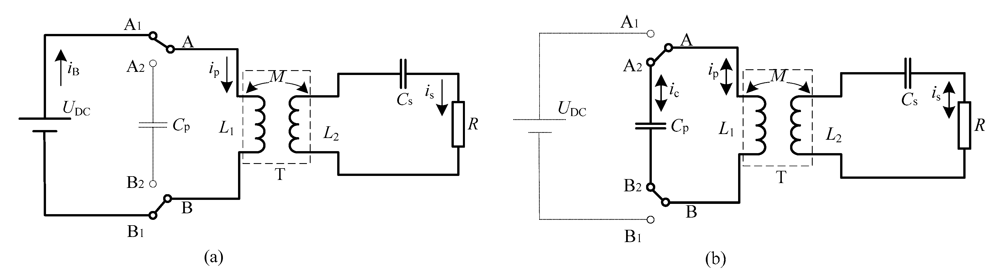
2.1. Basic Structure of the IIEIFR IPT System

A conceptual sketch of the IIEIFR IPT system is shown in Figure 1. In Figure 1, U_DC is the power source; T is the loosely coupled transformer consisting of the primary inductor L₁ and the secondary inductor L₂; M is the mutual inductance between the primary side and secondary side; C_p is the primary resonant capacitor; C_s is the secondary compensation capacitance; R is the load resistance; K₁ and K₂ are both double-throw switches.

According to the connection conditions of K₁ and K₂, the working process of the IIEIFR IPT system can be divided into two stages: the energy injection stage and the free resonance stage.

In the energy injection stage, as shown in Figure 2a, point A and point B are connected to point A₁ and point B₁, respectively; U_DC is connected to L₁ and C_p is isolated. Therefore, the current i_B flows into the primary inductor, there is i_B = i_p, and the energy is injected independently into the primary inductor. In this stage, the magnetic energy of the primary inductor increases, while part of the energy is transferred to the secondary side through the mutual inductance M.

In the free resonance stage, as shown in Figure 2b, point A and point B are connected to point A₂ and point B₂, respectively; C_p is connected to L₁ to form a resonant tank and U_DC is isolated, there is i_c = i_p. In this stage, the energy is continuously transferred to the secondary side and the IPT system can be regarded as working under the parallel-series resonance compensation mode.

2.2. System Modeling

In the energy injection stage, the primary conductor L₁ is connected to U_DC. Using the coupled mutual inductance model of the transformer, Figure 2a can be transformed as Figure 3. In Figure 3, i_p is the primary current, i_s is the secondary current. The controlled voltage source $Md{i}_{\mathrm{s}}/dt$ comes from i_s in the primary side, and the controlled voltage source $Md{i}_{\mathrm{p}}/dt$ comes from i_p in the secondary side.

In an IPT system, the mutual inductance M varies with the air gap. For convenience, M is usually described as coupling coefficient k, and there is

$$k=\frac{M}{\sqrt{L_1{L}_2}}$$

(1)

In the free resonance stage, L₁ is connected to the primary capacitor C_p. Using the coupled mutual inductance model of the transformer, Figure 2b can be transformed as Figure 4. In Figure 4, C_p and L₁ form the primary resonance network, C_s and L₂ form the secondary resonance network.

3. The IIEIFR IPT Power Converter

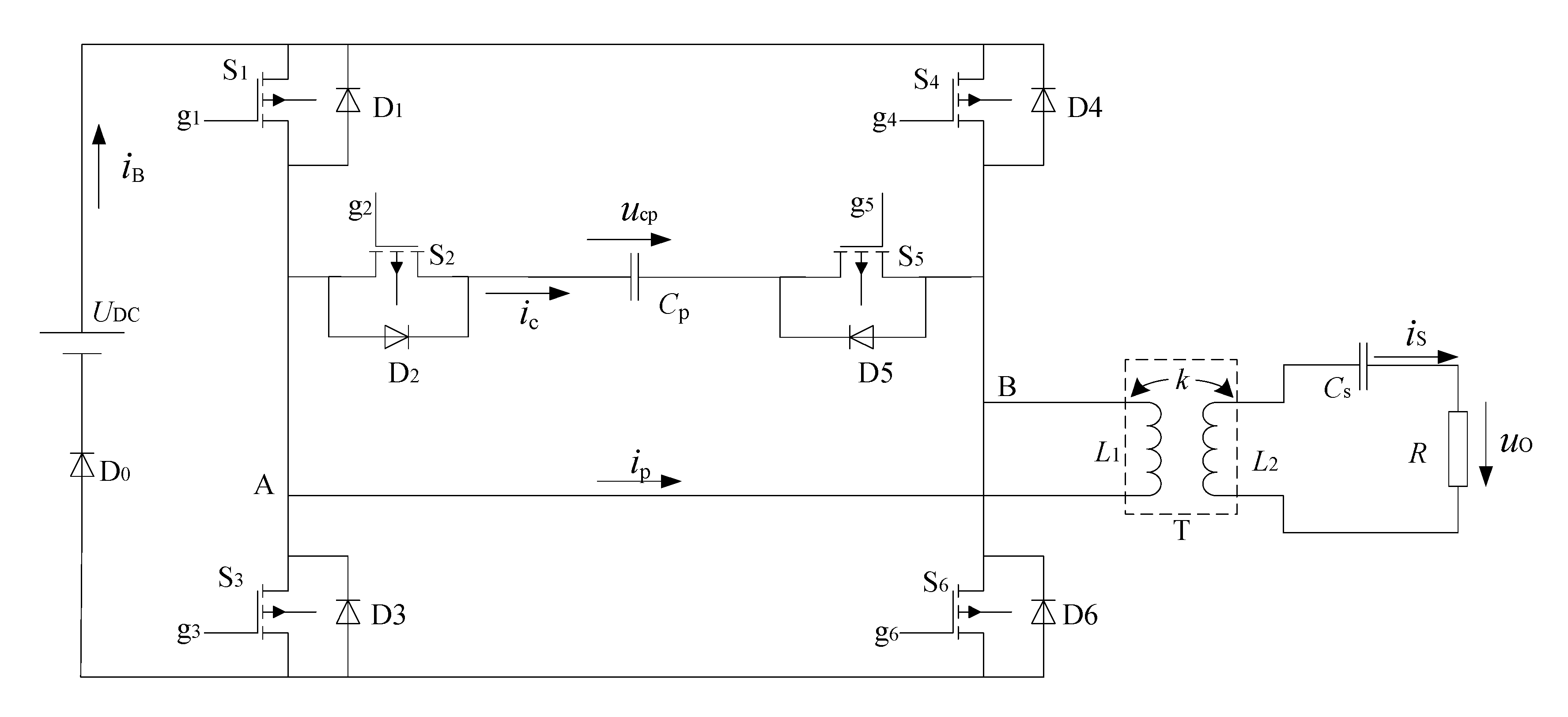
3.1. Topology of the IIEIFR IPT System

The topology of the IIEIFR IPT system is shown in Figure 5. In Figure 5, U_DC is the power source. Switches S₁, S₃, S₄, and S₆ form an H bridge, and the primary inductor L₁ is connected to point A and B of the H bridge. In addition, a resonant capacitor C_p is connected to point A and B through switches S₂, and S₅. Apparently, switches S₁ and S₂ play the role of K₁ in Figure 1. S₄ and S₅ play the role of K₂ in Figure 1. D₁ ~ D₆ are the parasitic diodes of S₁~S₆, respectively. D₀ is an anti-backflow diode. k is the coupling coefficient of the loosely coupled transformer, and R is the load resistor.

When S₁, S₆ are turned on and S₃, S₄, S₅ turned off, L₁ will be connected to U_DC. U_DC injects energy into L₁ through S₁ and S₆, and the system enters the energy injection stage. As i_p flows in the forward direction, this energy injection process is called the forward energy transfer period. On the other hand, when S₃, S₄, are turned on, and S₁, S₂ S₆ turned off, energy is injected into L₁ through S₃ and S₄, and the system enters the energy injection stage with i_p flowing in the reverse direction, which is called the reverse energy transfer period.

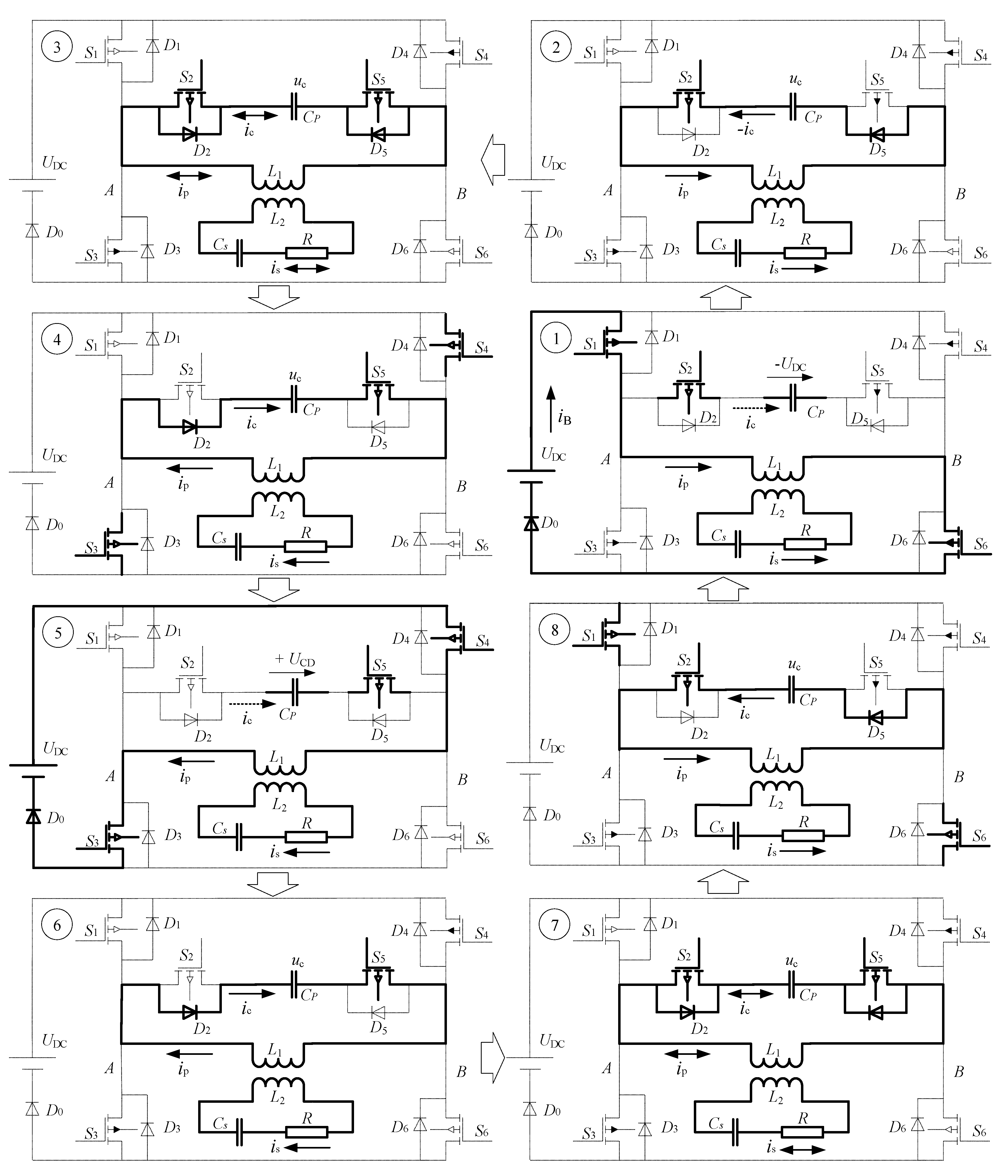
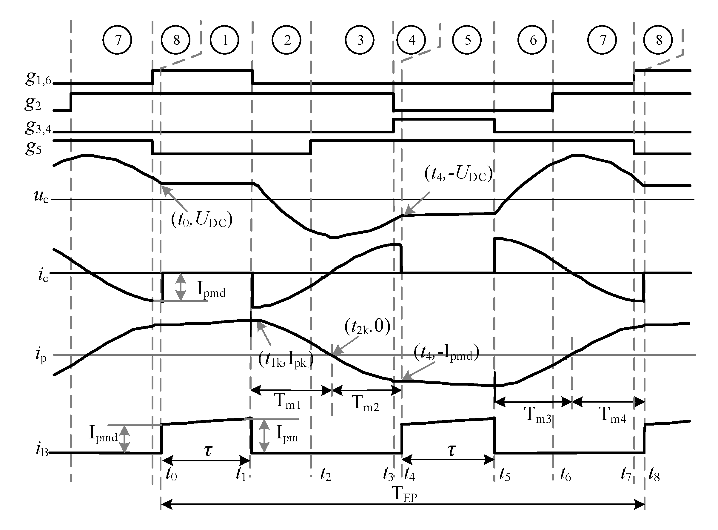
3.2. State Transition Analysis

As shown in Figure 6, an energy transfer process of the proposed converter can be divided into 8 working states, 4 for the forward energy transfer period and the other 4 for the reverse energy transfer period. The state transition sequence is indicated by state numbers from ① to ⑧. In the forward energy transfer period, state ① is the forward energy injection state, state ② is a transitional state from energy injection stage to free resonance stage, state ③ is free resonance state and state ④ is a transitional state from free resonance stage to reverse energy injection stage. States ⑤ ~ ⑧ are corresponding to the reverse energy transfer period, and the working principle is similar to the states ① ~ ④. In the schematic diagrams, the current-carrying devices and circuits are indicated by solid black lines. The voltage-blocking devices and circuits are indicated by a dotted line.

The waveforms of the i_B, i_p, i_c and u_cp are shown in Figure 7, where i_B is the current of U_DC, i_p is the current of L₁, i_c is the current of C_p, and u_cp is the voltage of C_p. In addition, g_1,6, g₂, g_3,4, g₅ are the control signals of switches. These signals are generated by the control strategy of the proposed converter. The state numbers are also shown in Figure 7.

In Figure 7, the time interval [t₀, t₄] is the forward energy transfer period, and from t₄ to t₈ is the reverse energy transfer period. In the forward energy transmission period, the interval [t₀, t₁] is the energy injection stage, which is corresponding to state ①, and the interval [t₁, t₄] is the free resonance stage, which is corresponding to states ②, ③ and ④.

As shown in Figure 6 and Figure 7, the working principles and fundamental equations of different states are shown as follows:

In state ①, S_1,6 have been turned on before moment t₀, i_p is provided by i_B, U_DC injects energy into L₁ independently through S_1,6 and D₀. As shown in Figure 3, the current and voltage equations of state ① can be written as

$$\{\begin{array}{c}{U}_{DC}=L_1\frac{d{i}_p}{dt}+M\frac{d{i}_s}{dt}\\ M\frac{d{i}_p}{dt}=L_2\frac{d{i}_s}{dt}+R{i}_s+\frac{1}{C_s}{{\displaystyle \int }}^{}{i}_{s}dt\end{array}$$

(2)

Assuming that t₀ = 0, the initial conditions can be obtained:

$$\{\begin{array}{c}{i}_p\left(0\right)={\mathrm{I}}_{pmd}\\ \frac{d{i}_p}{dt}|t=0=\frac{U_{DC}}{\left(1-k^2\right)L}\\ \frac{d{i}_p^2}{d{t}^2}|t=0=0\end{array}$$

(3)

Assuming L = L₁ = L₂, from Equations (1) and (3), the solution of Equation (2) is:

$$i_p=I_{pmd}+\frac{2\alpha k^2}{\left({\alpha }^2+{\omega }^2\right)\left(1-k^2\right)L}{U}_{DC}+e^{-\alpha t}\frac{k^2{U}_{DC}\sqrt{{\left({\omega }^2-{\alpha }^2\right)}^2+{\left(2\alpha \omega \right)}^2}}{\left({\alpha }^2+{\omega }^2\right)\left(1-k^2\right)\omega L}\sin \left(\omega t+{\theta }_i\right)+\frac{U_{DC}}{L}t$$

(4)

where

$$\{\begin{array}{c}\alpha =\frac{R}{2\left(1-k^2\right)L}\\ \omega =\sqrt{\frac{1}{\left(1-k^2\right)L{C}_p}}\\ {\theta }_i=\arctan \frac{2\alpha \omega }{{\omega }^2-{\alpha }^2}\end{array}$$

(5)

Considering that in applications such as EV charging, the IPT system usually works with low coupling coefficients (k < 0.3) [26], the second and third terms in Equation (4) can be neglected, and Equation (4) can be written as

$$i_p=I_{pmd}+\frac{U_{DC}}{L_1}t$$

(6)

From Equation (6), it is shown that during the energy injection stage, i_p increases linearly, and the rising slope is related to the primary inductance and U_DC.

In state ②, S₁, S₆ are turned off at moment t₁, and S₂ has been turned on before moment t₁, i_B drops to zero, and i_p is provided by i_c. In this state, C_p and L₁ form a resonance tank through S₂, D₅. The system begins to resonate freely, and i_p decreases sinusoidally from positive amplitude I_pm, where I_pm is the amplitude of i_p at time moment t₁. As shown in state ② of Figure 6, i_p can only flow in one direction. In order to form a free-resonating tank, S₅ needs to be turned on to allow i_p to flow bidirectionally before i_p become negative at moment t_k2. Therefore, an appropriate t₂ could be chosen at any moment in [t₁, t_k2]. That is, switch S₅ has a soft switch time margin as T_m1 = [t₁, T_k2].

In state ③, as t₂, S₂, S₅ are both “on”, the system resonates and i_p decreases sinusoidally.

State ④, [t₃, t₄] is a transitional state from the free resonance stage to the energy injection stage of the reverse energy transfer period. At moment t₃, switch S₂ is turned off, and i_p can only flow reversely. The automatic stage transition happens in this state and is explained as follows: As shown in Figure 7, switches S₃ and S₄ were turned on at time moment t₃, corresponding to state ④ in Figure 6. As shown in Figure 6, as there is a negative voltage on the capacitor C_p, the absolute value of which is larger than U_DC, therefore the diode D₀ is blocked and there is no current flowing out of the voltage source U_DC. When the absolute voltage on the capacitor C_p decreases to U_DC at t₄, the diode D₀ is unblocked and the voltage source starts to charge the inductor again. The system transits to the energy injection stage automatically.

As shown in the “u_c” curve in Figure 7, the start moment of the free resonance stage is when u_c equal to U_DC and the end moment is when u_c equal to –U_DC. Therefore, the free resonance stage basically lasts for half a cycle. As there is no switching action to trigger the stage transition, the switching action can be advanced of the stage transition and becomes flexible on the time. Therefore, by taking advantage of this automatic stage transition between the free resonance stage and the energy injection stage, the problem in determining state transition time in literature [25] is solved.

In Figure 7, it can be seen that in the interval [t_2k, t₄], i_p flows reversely. D₂ is turned on and a soft switching condition is formed to turn off S₂. In addition, in the same interval, i_B = 0, in which a soft switching condition is formed for S₃, S₄ to be turned on. This means that S₂, S₃, and S₄ have a soft switching time margin T_m2 = [t_2k, t₄]. In this time margin, an arbitrary moment can be chosen as t₃ to turn on S₃, S₄ and turn off S₂.

The free resonance stage including states ②, ③ and ④ can be analyzed as a whole in Figure 4. Assuming C = C_p = C_s, the voltage equations in [t₁, t₄] are shown as

$$\{\begin{array}{c}M\frac{d{i}_s}{dt}=L\frac{d{i}_p}{dt}+\frac{1}{C}{{\displaystyle \int }}^{}{i}_{p}dt\\ M\frac{d{i}_p}{dt}=L\frac{d{i}_s}{dt}+\frac{1}{C}{{\displaystyle \int }}^{}{i}_{s}dt+R{i}_s\end{array}$$

(7)

The solution of Equation (7) can be obtained using the method in the literature [20], there is

$$i_p=I_{pm}{e}^{-\alpha t}\sin \left(\omega t+\theta \right)$$

(8)

where I_pk is the peak amplitude of i_p in the free resonance stage. It means that, after moment t₁, C_p continues to provide current for L₁ in a short time and i_p reaches the peak amplitude of I_pk at moment t_1k. As the energy stored on C_p is very small, I_pk is approximately equal to I_pm Assuming I_pmd is the amplitude of i_p at time moment t₄, the difference between amplitudes of I_pm and I_pmd shows that in free resonance stage, energy is sent to the secondary side.

States ⑤–⑧ are the reverse energy transfer period, its working procedure is similar as the forward energy transfer period. The differences are that the polarity of the voltage and the direction of the current are opposite, as can be seen in Figure 6 and Figure 7.

According to the state transition analysis, compared with the traditional IPT topology, the energy injection and free resonance state are separated from each other, and there are certain time margins (T_m1, T_m2) at the switching time, which does not need to switch immediately at the zero crossing point of the primary current.

3.3. The Calculation of Parameters

3.3.1. The Amplitude and Phase Angle of Primary Current

There are two unknown values in Equation (8), amplitude I_pk and phase angle θ. As in the free resonance stage, t₄ − t₁ = π/ω, and I_pk = I_pm, there is

$$I_{pmd}=I_{pm}{e}^{-\alpha \frac{\pi }{\omega }}$$

(9)

Assuming the energy injection time τ = t₁ − t₀, and t₀ = 0, there is i_p(t₁) = I_pm. According to Equations (6), (8) and (9), there are

$$\{\begin{array}{c}{I}_{pmd}=\frac{U_{DC}}{(e^{{\alpha }_r\frac{\pi }{{\omega }_r}}-1)L_1}\tau \\ I_{pm}=\frac{U_{DC}}{(1-e^{-{\alpha }_r\frac{\pi }{{\omega }_r}})L_1}\tau \\ \theta =\frac{\pi }{2}\end{array}$$

(10)

3.3.2. The Energy Injection Time

As shown in Figure 7, in one energy transfer period, T_EP, there are two free resonance stages which both maintain half a cycle and two energy injection stages. There is

$${\mathrm{T}}_{\mathrm{EP}}=2\left(\frac{\pi }{{\omega }_r}+\tau \right)$$

(11)

According to Equation (11), there is

$$\tau =\frac{{\mathrm{T}}_{\mathrm{EP}}}{2}-\frac{\pi }{{\omega }_r}$$

(12)

3.4. Output Power

In state ①, i_p reaches its peak amplitude at t₁. According to the Equations (6) and (10), there is

$$i_p\left(t_1\right)=I_{pmd}+\frac{U_{DC}}{L_1}\tau =I_{pm}$$

(13)

The energy injected into the primary inductor during State ① can be calculated as

$$W_{\mathrm{m}}=\frac{1}{2}{L}_1{I}_{pm}^2$$

(14)

Considering that all switches operate under soft switching conditions, the power loss of the converter is neglected, and all the energy injected in primary side is transferred to the secondary side. Therefore, from Equations (10), (11) and (14), the output power can be obtained as

$$P_{\mathrm{o}}=\frac{W_{\mathrm{m}}}{{\mathrm{T}}_{\mathrm{EP}}}=\frac{{\omega }_r{L}_1{e}^{2{\alpha }_r\frac{\pi }{{\omega }_r}}{\left(\frac{U_{DC}}{L_1}\tau \right)}^2}{(e^{{\alpha }_r\frac{\pi }{{\omega }_r}}-1)\left(\pi +{\omega }_r\tau \right)}$$

(15)

4. Experimental Verification

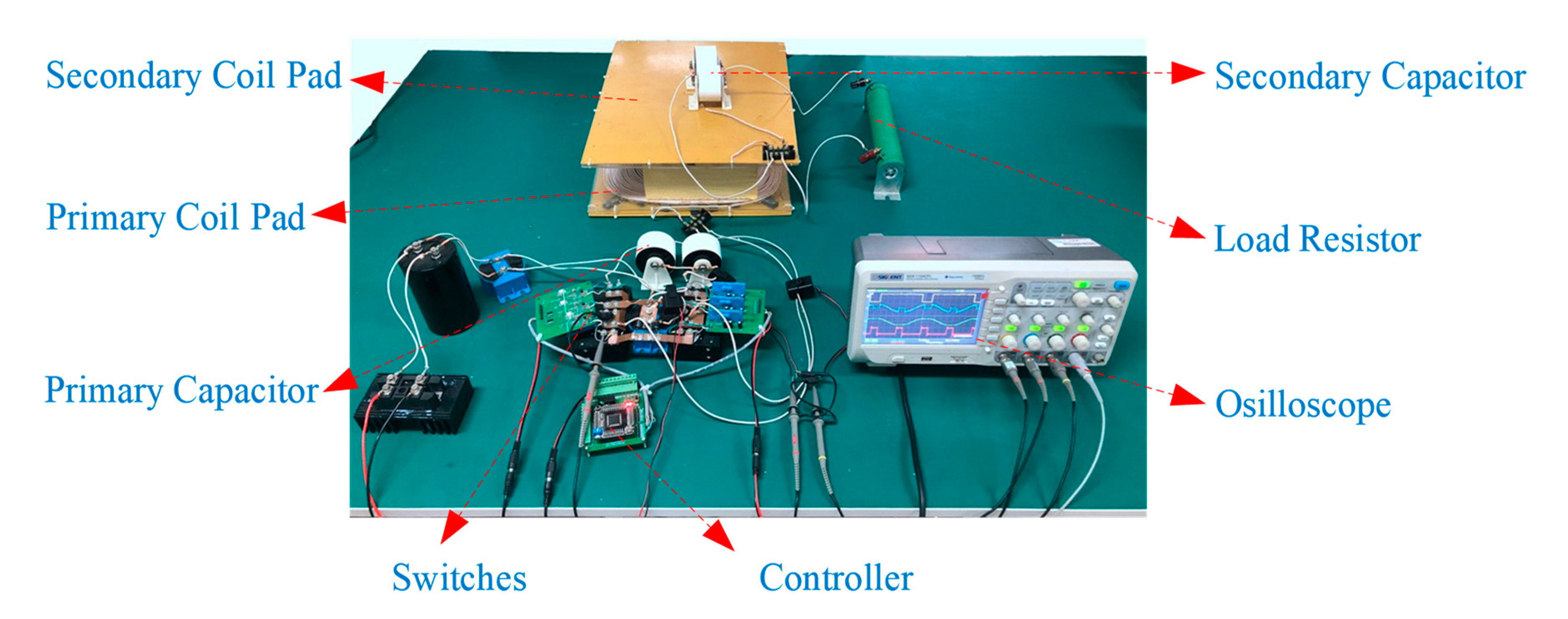
4.1. The Experimental Prototype

An experimental prototype was built to verify the proposed converter and control strategy of the IPT system. The system comprises of a converter, a loosely coupled transformer, a controller, and a load resistor, as shown in Figure 8. The values of the main parameters in the experiment are listed in

Table 1. The value of the component used in the prototype.

Parameter	Value
UDC	100 V
Cp, Cs	0.88 μF
L1, L2	640 μH
R	10–40 Ω
S1–6	IXFN56N90

. In the experiments, an oscilloscope (SDS 1104CFL, SIGLENT, Suzhou, China) and a power analyzer (WT500, YOKOGAWA Co, Tokyo, Japan) are used to measure the experimental results.

A pair of coil pads was used as the loosely coupled transformer. The detailed design of the coil pads has been shown in literature [25]. The inductance of the pads is 640 μH, and the mutual inductance between the pads varies with the air gap. Therefore, the coupling coefficient k also varies with the air gap h, and the relationship between them is shown in Figure 9.

4.2. Experimental Results

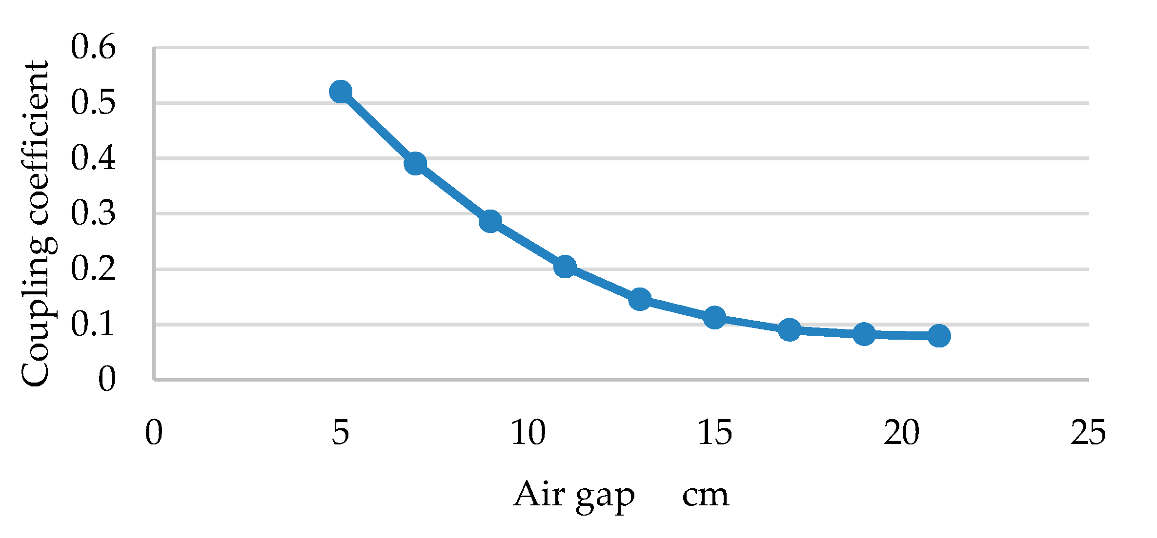
4.2.1. Features of the IIEIFR IPT System

The simulation and experimental results under U_DC = 100 V, R = 20 Ω, and h = 9 cm are shown in Figure 10. In Figure 10b, the source current i_B is the shallow blue curve, the capacitor current i_c is the purple curve, the red curve is i_p, and the blue curve is the control voltage of u_g1 and u_g2. From Figure 10, it is shown that the simulation and experimental results are consistent and well matched with the analytic results shown in Figure 7.

As shown in Figure 10, in the time interval [t₀, t₁], the system is in the energy injection stage, i_p = i_B and i_c = 0. It can be seen that i_p and i_B rise in this stage. At the end of this stage, both the simulation and experimental results of current i_p reached about 15 A, and the theoretical result from Equation (10) is 14.67 A, which indicated that the results of calculation, simulation, and experiment were consistent. In time interval [t₁, t₄], the system is in the free resonance stage. It can be seen that in this stage i_p decreases sinusoidally. i_p = −i_c, and i_B = 0. Notice that the free resonance maintains half a cycle in the interval [t₁, t₄]. At the end of this stage, both the simulation and experimental results of current i_p reached about 11 A, and the theoretical result is 10.72 A. It is shown that the simulation and experimental results were very close to the theoretical results.

It is also shown in Figure 10a that at the time moment t₇, switches S₁ and S₆ were turned on before the system entering the energy injection stage at t₈(t₀). However, i_B kept at zero until t₈; that is, there is a time difference Δt between the time that S_1,6 was turned on and the system stated the energy injection mode. The results verify that the system can automatically switch from the free resonance mode to the energy injection mode and the time margins analysis.

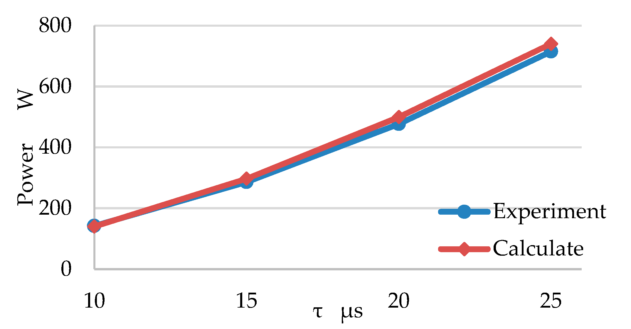
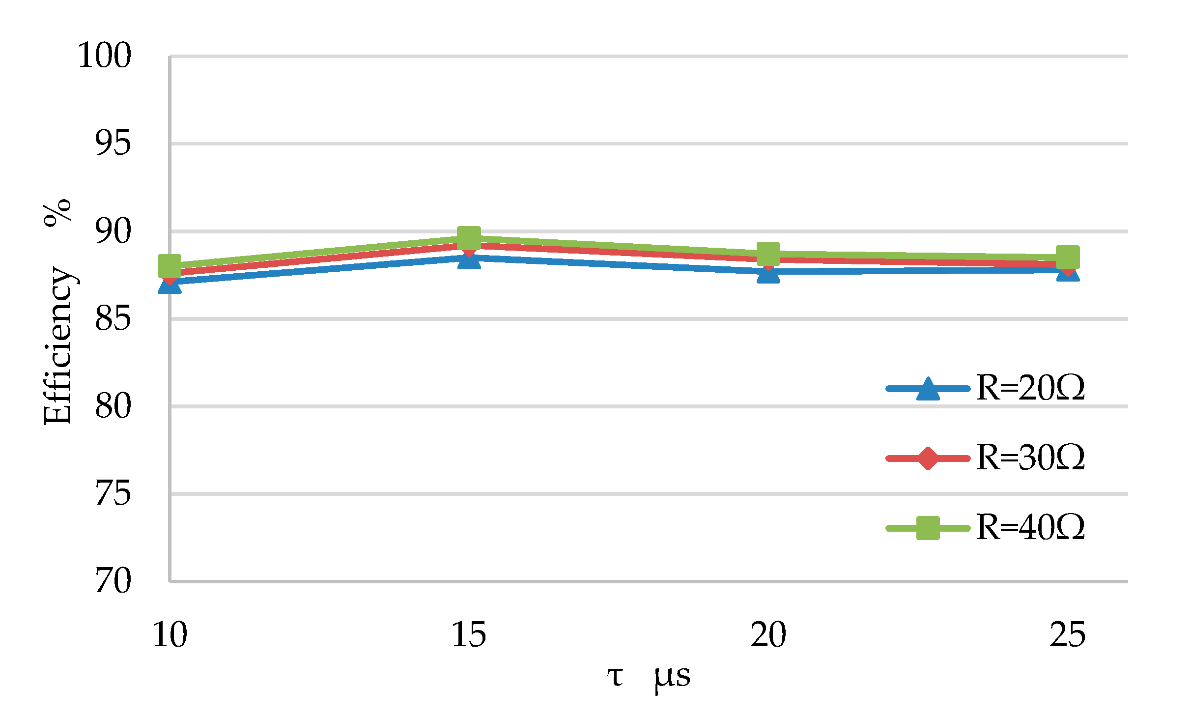
4.2.2. Power Control

The output power versus τ under the conditions of h = 9 cm, U_DC = 100 V, and R = 20 Ω is shown in Figure 11 as the blue line. When τ = 10 μs, the output power is 142 W, when τ = 25 μs, the output power is 715 W. As τ increases, the output power increases too. It is verified that the power can be regulated by energy injection time τ, and it also verified that the energy injection stage is separated from the free resonance stage which is different from the traditional control in IPT. For comparison, the output power calculated by Equation (15) is also shown as the red line in Figure 11. There is a small difference between the experimental and the theoretical results. This difference may be caused by the neglect of two components in Equation (4).

The efficiencies versus τ under different R are shown in Figure 12. It can be seen in Figure 12 that the curves when R is 20 Ω, 30 Ω and 40 Ω are very close, which implies that the load resistor has very small influence on the efficiency. When τ increases from 10 μs to 25 μs, there is a small variation on the efficiency. The minimum efficiency is 87.1%. The maximum efficiency is 89.6%, which implies that τ has very small influence on the efficiency.

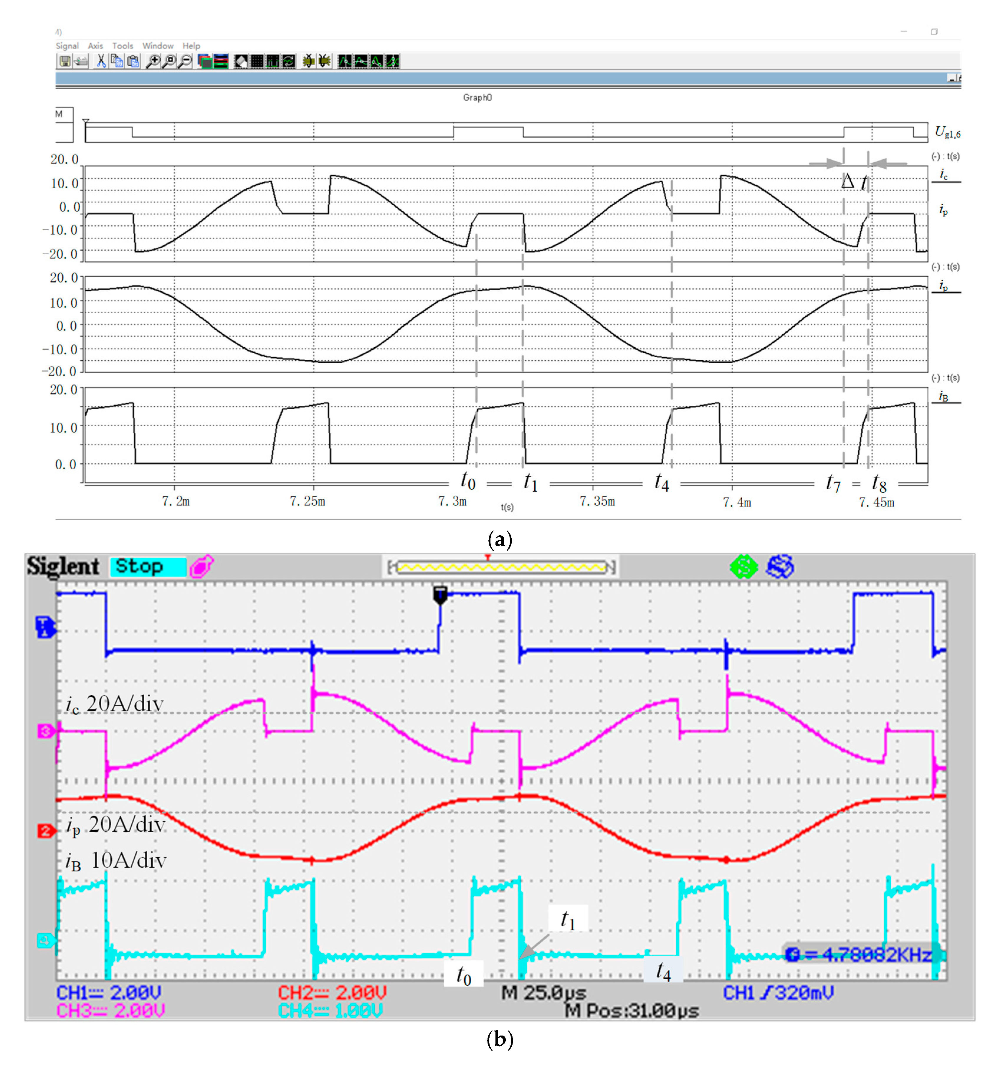
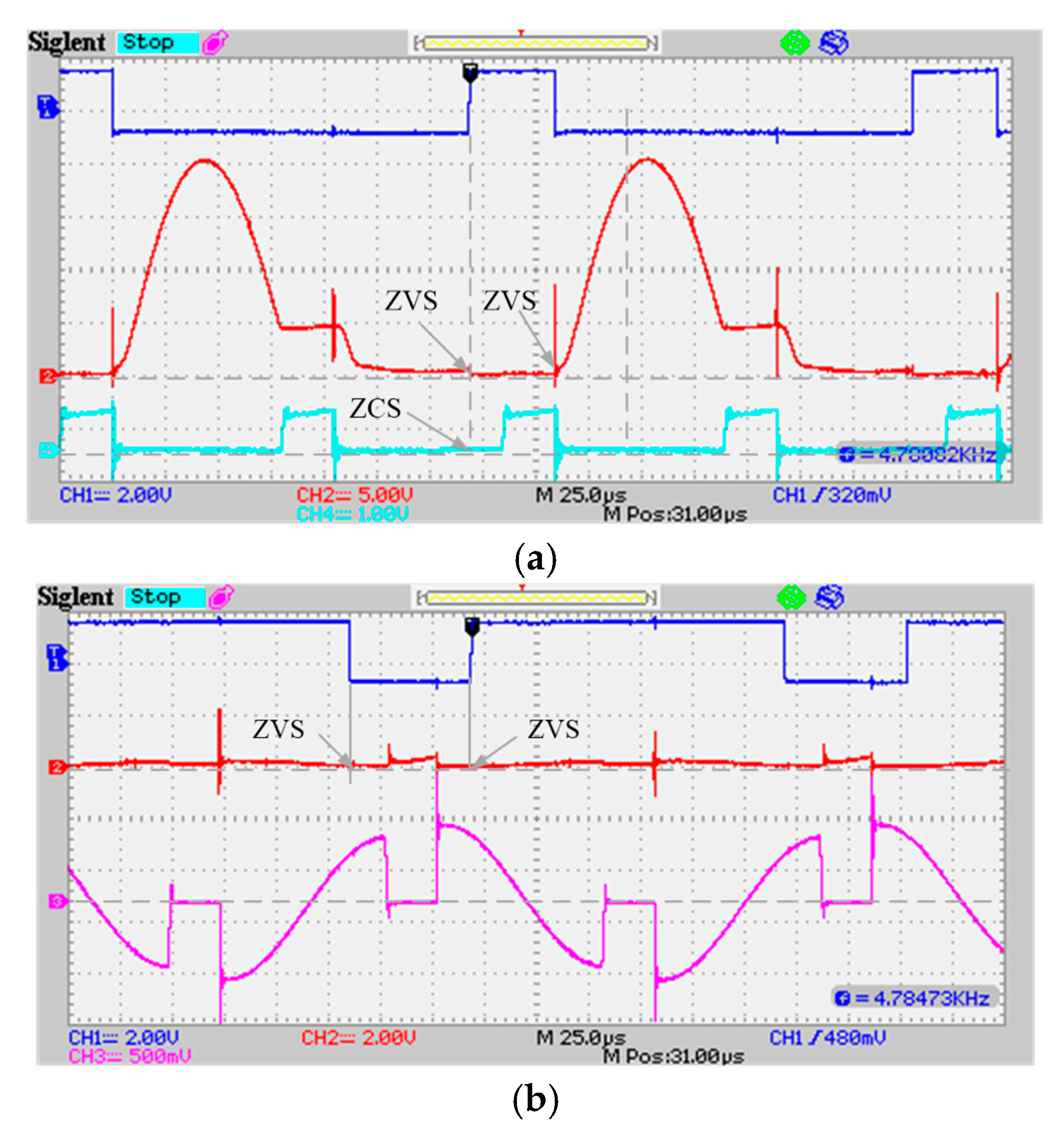
4.2.3. Soft Switching Condition

The voltage and current of switches S₁ and S₂ are shown in Figure 13. In Figure 13a, the control voltage of g₁ is shown as the blue curve; the voltage of u_s1 is shown as the red curve; and the current passing through switch S₁, i_s1 is shown as the shallow blue curve. From Figure 13a, the voltage u_s1 and current i_s1 are both zero when S₁ was turned. Therefore, switch S₁ is turned on under both zero voltage switch (ZVS) and zero current switch (ZCS) conditions. When S₁ was turned off, the voltage u_s1 was zero. Therefore, S₁ was turned off under ZVS condition. The switching condition of switches S₃, S₄, and S₆ are similar to S₁.

In Figure 13b, the blue curve is g₂, the control signal of S₂; the red curve is u_s2, the voltage of S₂; and the shallow blue curve is i_s2, the current of S₂. As shown in Figure 13b, the voltage u_s2 is nearly zero throughout the period. Therefore, whether S₂ has been turned on or off, its operation is under the ZVS condition. The switching condition of switch S₅ is similar to S₂.

5. Conclusions and Discussion

In an IIEIFR IPT system, the converter was decoupled from the resonant network, which can avoid the problem of frequency detuning and control the power easily. In this paper, the converter employed a novel control strategy with automatic stage transition. By this control strategy, the converter can automatically switch from the free resonance stage to the energy injection state without any switching actions. The free resonance stage will last for half a cycle no matter how the resonant frequency changes. Another advantage of the automatic state transition control is that it provides large time margins for switches under soft switching conditions, which make the switching time very flexible.

A prototype of IPT converter was built to drive the IPT system. The experimental results show that under the conditions of U_DC = 100 V, R = 20 Ω, and h = 5 ~ 11 cm, the operations of the converter were consistent with the theoretical analysis. The automatic stage transition phenomenon is shown along with all switches operated under soft switching conditions. When the energy injection time was adjusted from 10 μs to 25 μs the power changed from 143 W to 740 W, while the efficiencies were maintained between 87.1% and 89.6%.

Although the proposed control strategy shown in this paper has shown some merits in soft switching, during free resonance, the power supply does not inject energy into the system, so the transfer power density is lower than that of traditional IPT system. In the future work, we will try to improve the transmission power density of the system.

References

1. Zhong, W.; Lee, C.K.; Hui, S.Y.R. General analysis on the use of tesla’s resonators in domino forms for wireless power transfer. IEEE Trans. Ind. Electron. 2013, 60, 261–270. [Google Scholar] [CrossRef]
2. Steckiewicz, A.; Stankiewicz, J.M.; Choroszucho, A. Numerical and circuit modeling of the low-power periodic WPT systems. Energies 2020, 13, 2561. [Google Scholar] [CrossRef]
3. Barman, S.D.; Reza, A.W.; Kumar, N.; Karim, M.E.; Munir, A.B. Wireless powering by magnetic resonant coupling: Recent trends in wireless power transfer system and its applications. Renew Sustain. Energy Rev. 2015, 51, 1525–1552. [Google Scholar] [CrossRef]
4. Lee, S.-H.; Kim, J.-H.; Lee, J.-H. Development of a 60 kHz, 180 kW, Over 85% Efficiency Inductive Power Transfer System for a Tram. Energies 2016, 9, 1075. [Google Scholar] [CrossRef]
5. Campi, T.; Cruciani, S.; Feliziani, M. wireless power transfer technology applied to an autonomous electric UAV with a small secondary coil. Energies 2018, 11, 352. [Google Scholar] [CrossRef]
6. Lu, Y.; Ma, D.B. Wireless power transfer system architectures for portable or implantable applications. Energies 2016, 9, 1087. [Google Scholar] [CrossRef]
7. Kim, C.G.; Seo, D.H.; You, J.S.; Park, J.H.; Cho, B.H. Design of a contactless battery charger for cellular phone. IEEE Trans. Ind. Electron. 2001, 48, 1238–1247. [Google Scholar] [CrossRef]
8. Ibrahim, M.; Pichon, L.; Bernard, L.; Razek, A.; Houivet, J.; Cayol, O. Advanced modeling of a 2-kW series–series resonating inductive charger for real electric vehicle. IEEE Trans. Veh. Technol. 2015, 64, 421–430. [Google Scholar] [CrossRef]
9. Villa, J.L.; Sallan, J.; Osorio, S.J.F.; Llombart, A. High-misalignment tolerant compensation topology for icpt systems. IEEE Trans. Ind. Electron. 2012, 59, 945–951. [Google Scholar] [CrossRef]
10. Choi, S.Y.; Gu, B.W.; Jeong, S.Y.; Rim, C.T. Advances in wireless power transfer systems for roadway-powered electric vehicles. IEEE J. Emerg. Sel. Top. Power Electron. 2014, 3, 18–36. [Google Scholar] [CrossRef]
11. Zheng, C.; Ma, H.; Lai, J.S.; Zhang, L. Design considerations to reduce gap variation and misalignment effects for the inductive power transfer system. IEEE Trans. Power Electron. 2015, 30, 6108–6119. [Google Scholar] [CrossRef]
12. Cirimele, V.; Diana, M.; Freschi, F.; Mitolo, M. Inductive power transfer for automotive applications: State-of-the-art and future trends. IEEE Trans. Ind. Appl. 2018, 54, 4069–4079. [Google Scholar] [CrossRef]
13. Matysik, J.T. The current and voltage phase shift regulation in resonant converters with integration control. IEEE Trans. Ind. Electron. 2007, 54, 1240–1242. [Google Scholar] [CrossRef]
14. Gati, E.; Kampitsis, G.; Manias, S. Variable frequency controller for inductive power transfer in dynamic conditions. IEEE Trans. Power Electron. 2017, 32, 1684–1696. [Google Scholar] [CrossRef]
15. Matysik, J.T. A new method of integration control with instantaneous current monitoring for class D series-resonant converter. IEEE Trans. Ind. Electron. 2006, 53, 1564–1576. [Google Scholar] [CrossRef]
16. Moghaddami, M.; Sundararajan, A.; Sarwat, A.I. A power-frequency controller with resonance frequency tracking capability for inductive power transfer systems. IEEE Trans. Ind. Appl. 2018, 54, 1773–1783. [Google Scholar] [CrossRef]
17. Miller, J.M.; Onar, O.C.; Chinthavali, M. Primary-side power flow control of wireless power transfer for electric vehicle charging. IEEE J. Emerg. Sel. Top. Power Electron. 2015, 3, 147–162. [Google Scholar] [CrossRef]
18. Madawala, U.K.; Neath, M.; Thrimawithana, D.J. A power–frequency controller for bidirectional inductive power transfer systems. IEEE Trans. Ind. Electron. 2013, 60, 310–317. [Google Scholar] [CrossRef]
19. Berger, A.; Agostinelli, M.; Vesti, S.; Oliver, J.A.; Cobos, J.A.; Huemer, M. A wireless charging system applying phase-shift and amplitude control to maximize efficiency and extractable power. IEEE Trans. Power Electron. 2015, 30, 6338–6348. [Google Scholar] [CrossRef]
20. Dede, E.J. Improving the efficiency of IGBT series-resonant inverters using pulse density modulation. IEEE Trans. Ind. Electron. 2011, 58, 979–987. [Google Scholar] [CrossRef]
21. Fujita, H.; Akagi, H. Pulse-density-modulated power control of a 4 kw, 450 kHz voltage-source inverter for induction melting applications. IEEE Trans. Ind. Appl. 1996, 32, 279–286. [Google Scholar] [CrossRef]
22. Li, H.L.; Hu, A.P.; Covic, G.A. Development of a discrete energy injection inverter for contactless power transfer. In Proceedings of the 2008 3rd IEEE Conference on Industrial Electronics and Applications, Singapore, 3–5 June 2008; pp. 1757–1761. [Google Scholar] [CrossRef]
23. Li, H.L.; Hu, A.P.; Covic, G.A. A direct AC–AC converter for inductive power-transfer systems. IEEE Trans. Power Electron. 2012, 27, 661–668. [Google Scholar] [CrossRef]
24. Chen, L.; Hong, J.; Guan, M.; Wu, W.; Chen, W. A power converter decoupled from the resonant network for wireless inductive coupling power transfer. Energies 2019, 12, 1192. [Google Scholar] [CrossRef]
25. Chen, L.; Hong, J.; Guan, M.; Lin, Z.; Chen, W. A converter based on independently inductive energy injection and free resonance for wireless energy transfer. Energies 2019, 12, 3467. [Google Scholar] [CrossRef]
26. Sallán, J.; Villa, J.L.; Llombart, A.; Sanz, J.F. Optimal design of ICPT systems applied to electric vehicle battery charge. IEEE Trans. Ind. Electron. 2009, 56, 2140–2149. [Google Scholar] [CrossRef]
Figure 1. The conceptual sketch of the independent inductance energy injection and free resonance (IIEIFR) inductive power transfer (IPT) system.
Energies 13 05268 g001
Figure 2. Two-stage working procedure of the IIEIFR IPT system. (a) Energy injection stage. (b) Free resonance stage.
Energies 13 05268 g002
Figure 3. Equivalent circuit diagram of the IIEIFR system in the energy injection stage.
Energies 13 05268 g003
Figure 4. Equivalent model diagram in the free resonance stage.
Energies 13 05268 g004
Figure 5. The topology of the IIEIFR IPT system.
Energies 13 05268 g005
Figure 6. State transition of the IIEIFR IPT system ① The forward energy injection state, ② The transition state from the forward energy injection state to the forward free resonance state, ③ The forward free resonance state, ④ The transition state from the forward free resonance state to the reverse energy injection state, ⑤ The reverse energy injection state, ⑥ The transition state from the reverse energy injection state to the reverse free resonance state, ⑦ The reverse free resonance state, ⑧ The transition state from the reverse free resonance state to the forward energy injection state.
Energies 13 05268 g006
Figure 7. The waveforms of the IIEIFR IPT converter.
Energies 13 05268 g007
Figure 8. The prototype of the IPT system.
Energies 13 05268 g008
Figure 9. Coupling coefficient versus the air gap.
Energies 13 05268 g009
Figure 10. The simulation and experimental results of ip, ic, and iB. (a) Simulation results. (b) Experimental results.
Energies 13 05268 g010
Figure 11. The output power versus τ.
Energies 13 05268 g011
Figure 12. The curve of efficiencies versus τ under different load resistor.
Energies 13 05268 g012
Figure 13. The waves of switches. (a) S1. (b) S2.
Energies 13 05268 g013