Impact of DSM on Energy Management in a Single-Family House with a Heat Pump and Photovoltaic Installation

Abstract

This article presents a case study of a single-family house, whose current energy source is electricity only. Nine years ago, the heat source for the heating system and domestic hot water was an oil boiler, which was changed to an air–water heat pump. Four years ago, when Poland formed the basis of the prosumer market, the first photovoltaic system was established. It was expanded in the following years. In this work are presented the impact of using a heat accumulator on the coefficient of performance of the heat pump, the self-consumption of energy from the photovoltaic system, and the cost of purchasing energy. Comparative calculations were made, with the demand-side management (DSM) active on work days, and on free days (weekends and public holidays) it was not. Attention was paid to the self-consumption factor depending on the algorithms used in an energy meter. The prosumer market in Poland was also described. The calculations described the house as having an annual energy self-consumption from photovoltaic about 6% higher than average values obtained in buildings with heat pumps. Simultaneously, due to energy storage in heat and the load shifting in the multi-zone tariff, the cost of purchasing energy was 47% lower than in a single-zone tariff (without heat storage and load shifting).

1. Introduction

The European Union pursues a policy of reducing the use of energy produced from fossil fuels by determining individual countries’ targets for the share of renewable energy sources (RES) in their energy mix. The main problem associated with some renewable energy sources, such as photovoltaic (PV) and wind energy, is their variability. A solution would be large-scale energy storage. Another approach is also possible. Distribution system operators (DSOs) can shape electricity demand with several instruments, e.g., demand-side management (DSM) or demand-side request (DSR). The simplest variants of DSM are time-based programs offered as multi-zone tariffs. In certain hours of the day and on specific days of the week, lower energy prices are offered, which should encourage users to use energy during these times. From the DSOs point of view, the DSR system gives more possibilities, but it is more restrictive for energy users. A conducted simulation shows that the use of the DSR in a building with a heat pump (HP) could increase the auto consumption by 12%, while reducing energy costs by up to 30% [1]. However, in Poland, only big energy consumers can use the DSR [2].

In buildings with a photovoltaic system (PVS), the aim is to ensure that the self-consumption is as large as possible. At the same time, using locally stored energy, they can shift the peak load. Years ago, the economic profitability of energy storage was optimistically prognosed even without a support system; such process, however, is nowadays only presented in Germany [3]. Today’s data show that without support, such systems are unprofitable. The unit cost of an electric energy storage system (EESS) has not decreased to the optimistic level of 200 EUR/kWh [4].

From a technical point of view, the most advantageous energy storage solution on a small scale seems to be the EESS. However, in many countries, e.g., Poland, where electricity is relatively cheap, even with twice the energy price, the investment in the EESS will never pay off. In Poland, only certain other aspects may lead to the decision to install the EESS. Only some countries, such as Germany or Sweden for instance, employ the EESS in up to 60% of cases [5,6]. There ought to be a discussion as to whether an EESS increases the self-consumption and self-sufficiency, as demonstrated in many articles which will not be cited here.

An advantageous effect of energy accumulation is the stabilization of the operation of a DSO grid. The reduction in the amount of energy supplied to the DSO grid does not disturb its work, and does not cause a limitation of energy generation or even a disconnection of inverters. Inverters must respect the requirements of standards [7,8,9], and such an operation is increasingly observed.

This article presents the effects of the first version of the home energy management system (HEMS) that managed the highest load, the HP. The HP consumed 65% of the total annual energy of the building, and its consumption could be shifted outside of peaks hours. This is made possible by storing energy in heat, both in the domestic hot water buffer (DHWB) and in the heating buffer (HB). Optimizing the load shift had a negative impact on the energy self-consumption of the PVS. The results presented come from a real household. The proposed solution is as effective as the EESS, but the costs are significantly lower. The results are specific to PVSs cooperating with the HP. Keeping in mind that the initial incentive instruments for prosumers will be reduced and eliminated in coming years [10], one should look for ways to increase self-consumption. The described solution has two modernization aspects. The technical aspect shows the possibilities of the heating system (HS). The second aspect shows the economic merits of the applied solution.

2. The Genesis of the Study

2.1. Review of the Effectiveness of DSM Solutions

The DSM mechanism should encourage customers to reduce electricity peaks. This can be done by shifting loads. Unfortunately, most domestic consumers do not analyze the profitability of tariff changes, and thus are not aware of the opportunities this can provide. Although they have information on potential savings, this has proven insufficient to change their behavior. The financial incentive was able to shift ca. 3% of their consumption (a field study on more than 100 households was performed) [11]. The article’s [12] conclusions are that load shifting can potentially increase the PV’s self-consumption by a few percent of the total PV power generation (about 200 kWh in annual consumption).

The peak price of energy, which coincides with the maximum gain of energy from the sun, should prompt prosumers to increase their self-consumption. Most of the described solutions increase self-consumption based on the EESS and the DSM. For the battery capacities (in kWh) related to the peak power of the photovoltaic system (in kWp) in the range of 0.3–1, the results show that it is possible to increase self-consumption from 10% to 25%. The simultaneous use of the EESS and the DSM increases this to 30% [13].

There are a few studies which examine the effect of heat accumulation on self-consumption. The conclusions often show the advantage of the heat accumulation of energy over the EESS [14]. This is often presented via technical details, and not always by justifying economic legitimacy, in particular for the EESS [15].

The authors present many different algorithms. In the article [16], the authors, apart from proposing an algorithm for load shifting, also present a review of the used algorithms and their achievements and limitations. These are used load control algorithms based on load planning, load prediction, and binary backtracking search algorithms [17].

In summary, many proposed solutions do not consider the convenience, user comfort or energy consumption, and the optimalization of the peak-to-average ratio does not include the maximization of self-consumption. Therefore, it is not surprising that consumers are only slightly interested in adopting the DSM mechanism understood in this way. A reasonable compromise is needed, taking into account the convenience of using the equipment, mainly in household appliances.

2.2. Prosumer Support in Poland

In almost all European countries, there is prosumer support by feed-in tariff (FiT). In the initial period of introduction of the feed-in tariffs, they were so attractive that many investors invested their own funds into the construction of RES installations. With the increase of energy generation from the RES, the FiT gradually approached the standard tariffs of energy consumers, and in subsequent years it has declined [18,19]. This should prompt prosumers to increase their self-consumption [20].

In 2015, the next version of the RES Act [10] was enforced, which for the first time included prosumer provisions, which were to be applied from 2016. According to the Act, guaranteed tariffs should exist, differing depending on the power of the RES installations. Until then, prosumers could sell surplus energy for less than 50% of the average price of energy on the wholesale market. Unfortunately, a few days before the enforcement of the Act, it was amended [21]. Instead of FiTs, a rebate system has been introduced. As part of the rebate system, the prosumer can deliver energy to the DSO grids, and within one year withdraw 80% of the delivered energy for 10 kWp installations, or 70% for larger installations (not exceeding 50 kWp). The diagram of how the rebate system works is shown in Figure 1. This mechanism allows prosumers to move energy surpluses from spring and summer to autumn and winter. However, it is difficult to call this an accumulation of energy, but from the perspective of prosumers it works like that.

However, if the amount of energy transferred to the grid exceeds the amount of energy consumed, this difference will be transferred to the energy distributor free of charge. Therefore, it is not possible to balance electricity charges to zero, because fixed charges will always remain. Nor is it possible to generate additional profits from the sale of energy; this can only bring savings.

An important element of the RES Act [21] is net-metering, i.e., the method of settling the prosumer’s bidirectional energy transfers. For three-phase installations, the Act [21] introduced the obligation of balancing the energy taken and fed into the grid before its counting in the registers of the energy meter. How it is actually billed is shown in the next chapter.

2.3. Energy Meter Algorithms and Calculated Self-Consumption

The calculation of the self-consumption factor for the RES seems simple, using the DSO energy meter and the state of energy stored in an inverter or measured by an additional energy meter. No articles discussing self-consumption or determination mention the algorithms implemented in energy meters [22]. This is quite important because this algorithm affects the calculated self-consumption. The problem does not occur in the rare case when electric installation is single-phase. However, in a three-phase installation, the calculated self-consumption can be different from its true value. The reason for the discrepancy is the algorithm of the energy summation from the individual phases implemented in the meter. Prosumer meters are four-quadrant meters that count active and reactive energy in both directions. From four available algorithms, in most cases only two are selected. These are known as the vector summation mode, or Ferraris mode, and the algebraic summation mode. In Ferraris mode, the instantaneous power from three phases is summed first, accounting for the direction of energy flow. Then, the state of register counting the energy either imported (8.1.X (X is the register number for the time zones (1, 2, 3), for single-zone tariffs X = 0)) or exported (8.2.X) is increased depending on the resulting energy flow direction. According to the names used in the instructions for electric energy meters discussed in this article, the energy imported or exported means energy drawn from the grid or given to the DSO grid, respectively. In the algebraic summation mode, there is no summation of instantaneous power from the three phases, and the registers of energy imported (8.1.X) and energy exported (8.2.X) can be increased simultaneously, based on the instantaneous energy flow directions in each phase. Using the vector algorithm, the indications of counter registers (both import and export) will be lower than for the arithmetic algorithm, but the energy balance, i.e., import–export, will be the same. How different the results for both algorithms can be is shown in an example in Figure 2.

Although the energy balances are zero, there are differences in the calculated self-consumption ratios. For the vector mode, the calculated self-consumption factor is 100%, and for the algebraic mode it is only 33.3%. The time diagrams in Figure 3 show the measurements for an example day in March 2019. They were carried out simultaneously for two meters with both algorithms. The difference in calculated self-consumption is more than twofold. These two examples show the impact of the algorithm used in the meter on the calculated self-consumption factors.

Real energy flows reflect meters with algebraic mode. The self-consumption factor calculated on the basis of a vector mode energy meter is overstated. Unfortunately, it is not possible to convert the data obtained from a three-phase meter with a vector mode into readings in algebraic mode, and vice versa. This is because three-phase meters indicate only total energy from all phases. The self-consumption information should focus on the algorithm with which the energy meter operates. It is hard to compare the results without this knowledge.

Turning to the case study, when the considered building tariff was changed to G13 in the new energy meter at the end of 2019, the energy balancing was changed also, although the RES Act [21] was not changed. Such actions are taken not only by the local DSO, but also by other DSOs. In the opinion not only of the prosumers, but also of the Ministry of Energy, this is against the law. Prosumers feel the financial consequences of these actions, although their self-consumption does not change. This led to an impulse to take action to reduce the negative effects.

Tauron, the local DSO, has a specific billing system in multi-zone tariffs. In short, the cost of energy exported to the grid is equal to the average cost of energy imported from the grid, regardless of the time zone in which it is generated. How this is disadvantageous for prosumers is outlined in Section 4.3.

3. Limitations and Possibilities of Typical Automation of the Heating System and the Photovoltaic System

3.1. Heating System

In the single-family building, electricity is currently the only source of energy. The existing heating system (HS) scheme (Figure 4) differs from the scheme recommended by the manufacturer [23]. The heat pump manufacturer has provided one HB whose temperature is determined by the HS algorithm with higher temperature requirements.

Because the HP is the largest energy receiver, the first step was to achieve maximum heat cost savings. When analyzing the possibilities of HS control, many important restrictions were encountered, including:

• The controller allows one to program two heating circuits, but the temperature of only one can be controlled by a three-way valve;
• The HB temperature is determined by the weather control algorithm (heating circuit with a higher required temperature), or is defined as constant when the outside temperature falls below a selected setpoint;
• The electric power of the HP compressor cannot be remotely adjusted. It can only be turned on or off.

In the case of two heating circuits, these restrictions significantly limit the use of the HB as a heat accumulator. Due to the existence of two heating circuits, the floor and fan coil units, two buffers (HB 1 and HB 2) were used with different heating water end temperatures. The maximum temperature difference between the water supplying the fan coil and the floor circuits is 10 K. This difference is significant in terms of the COP of the HP and the amount of electricity needed to obtain the heat. For the three example points, the COPs are COP(A2/W35) = 3.25, COP(A2/W45) = 2.8, and COP(A2/W55) = 2.1. Thus, to store the same energy, at the end temperatures of 45 °C and 55 °C, 16% and 55% more electricity is needed, respectively, compared to 35 °C.

3.2. Photovoltaic System

The first PVS with 2.64 kW_p (marked PV1 in Figure 5) was built in March 2016. In January 2018, additional panels (PV2) of 0.54 kW_p were installed, and in April 2019 the system was extended by an additional 1.64 kW_p (PV3). The added panels PV2 and PV3 transfer energy to the grid using microinverters. Although the sum of the maximum power of the installed PV panels is 5.07 kW_p, the PVS achieved a maximum power of 3.25 kW. This is due to the lack of a sufficiently large south-facing area.

3.3. Energy Storage Capacity in Water Buffer Tanks

In the central part of the DHWB, the minimum temperature is 40 °C and the maximum is 50 °C. This temperature range was used for accumulation. It can store 15.9 MJ (4.4 kWh) of heat. There are two charge and discharge cycles per day. Considering the COP, this amount of heat requires from 2.8 kWh of electricity in summer to 4.8 kWh in winter (Figure 6).

The two HBs have greater capacities for heat accumulation due to their larger capacity and temperature range. It was assumed that the temperature in the HBs will be 20 °C higher than the set temperature, which for floor heating does not exceed 35 °C. This allows the accumulation of 50.3 MJ (14 kWh) with one charging. There are also two charging cycles per day. Given the COP, this amount of heat requires between 7.4 kWh and 13.6 kWh of electricity. In summer, this proportion can be increased on days with extremely high temperatures by switching the HP to the cooling mode and simultaneously storing the cold in buffers. Cooling only occurred when the PVS energy covered 100% of the HP electricity demand. The charge cycle occurs once per day. In this way, by chilling the water to 5 °C, 37.3 MJ (10.5 kWh) of cold can be accumulated, which is equivalent to between 3.1 kWh and 3.8 kWh of electricity (Figure 6).

The timings that control heat accumulation in the DHWB and the HBs on work days are shown in Figure 7. Examples of actual temperature changes in the tank HB 2 and the temperature of the water supplying the heating circuit are shown in Figure 8.

3.4. Costs of Investment in Heat Storage

This is a very simplified analysis of comparing the costs of energy storage in heat and electrochemical transformations.

Considering the net catalogue costs of Vitocell buffers [24], and additional installation and labor costs, the total investment cost including tax was EUR 3280, which gives 333 EUR/kWh per unit energy. It should be added that Viessmann products belong to the top price range. For comparison, the Tesla Powerwall 2 12.6 kWh was the cheapest EESS. Its cost, including installation, is about EUR 13,300 [25], which is 1090 EUR/kWh, i.e., three times more than for the thermal storage.

The heat storage can be used for 20 years without loss of capacity, and the manufacturer guaranteed a Powerwall durability of 10 years. With time, its capacity drops to 70% of its initial value. Assuming that on average 12 kWh would be accumulated daily, the cost of energy storage would be 0.037 EUR/kWh for heat storage and 0.31 EUR/kWh for the chemical batteries. The annual amortization (of 20 years’ lifetime) would increase the energy cost by EUR 82 for the heat storage and EUR 665 for the EESS. The analysis, although simplified, shows that the cost of investment in heat storage is four times lower than in electricity storage. Considering the cost of accumulated energy, the discrepancy is even greater, at eight-fold. This also results from the drop in battery capacity. Heat accumulation, although economically beneficial, does not allow for the use of stored energy other than as a heat source.

4. Data Analysis

4.1. Sources of Data

The results presented in the article are based on measurement data from the building over an almost 4-year period. The measurements of the energy imported and exported (Figure 9), generated by the PVS and consumed by building are split into various components, including the HP (Figure 10).

Based on these, two main indicators were determined, namely COP and self-consumption. These were calculated not only as annual indicators, but also for four specific cases: the heating season and the summer season, as well as work days and free days.

4.2. Household Energy Consumption

For further calculations, the structure of the monthly energy consumption in the building was analyzed. Figure 11 presents graphs split by the consumed energy (taken from the grid together with the PV self-consumption), the HS (pumps and automation), the DHW and the household in the following months of the year.

Table 1. Structure of energy use in seasons and year.

	Percentage Energy Consumption
	Heating Season	Summer Season	Annual Average
Heating	57.6	8.4	46.7
Household	20.7	59.6	29.3
Warm water	14.2	27.0	17.0
Heating system	7.5	5.0	7.0

shows the structure of energy consumption, in the same categories, per heating season, summer season, and as an average for the whole year. The heating season was adopted from October 1 to May 1. The rest of the year was defined as the summer season, although the heating was occasionally run on cool days in May and September. The heating of the building, the main energy consumer, uses up 59% of the energy used during the heating season, and 48% over the whole year. A significant part of the energy is used by the DHW—a 16% share of annual energy. Therefore, any action to reduce the energy components’ costs will be positive for users.

4.3. Energy Import and Export

The amount of energy imported to and exported from the grid was analyzed, considering the time zones of the G13 tariff, to allow for the results to be converted to another tariff. For further information from 2019, the average hourly profiles of imported and exported energies were determined, with a split between the heating and summer seasons and work and free days.

The daily average energy values for each time zone are given in

Table 2. Average daily imported energy in the summer and heating seasons for work days and free days.

Time Zone	Heating Season		Summer Season
	Work Days	Free Days	Work Days	Free Days
	kWh	kWh	kWh	kWh
Total	27.88	29.92	7.10	7.91
T1	1.31	0.00	0.30	0.00
T2	2.97	0.00	1.21	0.00
T3	23.60	29.92	5.59	7.91

. They are slightly lower on work days than on free days. The differences are slightly greater during the heating season, partly due to heat accumulation. In both cases, the differences are less than 5% of their average values. The import of energy from the grid in the heating season was almost four times higher than in the summer, due to the heating of the building and the much lower PV generation.

A similar analysis as in the case of exported energy was carried out for the imported energy. Average energy values in the heating and summer seasons for each time zone are given in

Table 3. The average daily exported energy in the summer and heating season for work days and free days.

Time Zone	Heating Season		Summer Season
	Work Days	Free Days	Work Days	Free Days
	kWh	kWh	kWh	kWh
Total	2.76	2.47	10.86	10.39
T1	2.09	0.00	6.04	0.00
T2	0.05	0.00	0.09	0.00
T3	0.63	2.47	4.74	10.39

. The average daily energy export in the summer season on work days was a bit greater than the energy exported on free days. Slight differences also occurred during the heating season; the energy export on work days was slightly higher than on free days. On average, the energy exported to the grid in the summer season was four times higher than in the heating period.

Table 4. Sum of imported and exported energy in the summer and heating seasons, and all year, for work days, free days and all days.

Time Zone	Import			Export
	Work Days	Free Days	All Days	Work Days	Free Days	All Days
	kWh	kWh	kWh	kWh	kWh	kWh
Total	4824	2347	7170	1554	651	2205
T1	222	0	222	944	0	944
T2	562	0	562	17	0	17
T3	4039	2347	6385	593	651	1245

shows the energy flows in both seasons, and

Table 5. Structure of imported and exported energy in the summer and heating seasons, and all year, for work days, free days and all days.

Time Zone	Import			Export
	Work Days	Free Days	All Days	Work Days	Free Days	All Days
	%	%	%	%	%	%
T1	4.6	0.0	3.1	60.8	0.0	42.8
T2	11.7	0.0	7.8	1.1	0.0	0.7
T3	83.7	100.0	89.1	38.2	100.0	56.4

shows the percentage structure of energy flows.

It is worth noting that almost 90% of the energy was imported in the T3 zone annually, while only slightly more than half of was exported in this time zone. Only 10% of the energy was imported in zones T1 and T2, and 43% was exported. There was almost no energy export in the T2 zone, indicating an almost 99% self-consumption in the afternoon. In the articles [26,27], a west-oriented PV installation is suggested. As can be seen, it is possible to obtain a large self-consumption this way, but this does not compensate for the much smaller energy obtained thereby.

The calculated average unit energy cost will be 0.073 EUR/kWh, considering the share of each tariff zone of the imported energy (Table 4) and the G13 tariff. For exported energy, it would theoretically be 0.086 EUR/kWh. The difference is 17%. At this point, it is worth recalling the unfavorable billing of prosumers via multi-zone tariffs, for which the cost of exported energy is assumed to be the same as that of imported energy.

5. Calculations and Results

5.1. Influence of Heat Accumulation on the Heat Pump’s COP and PV Energy Self-Consumption

The term self-consumption ratios is used many times in this article. The coefficients are determined for a period of one day, ${\mathsf{\Phi }}_D$, (Equation (1)), one month, ${\mathsf{\Phi }}_M,$ (Equation (2)) and, similarly according to Equation 2, for work days, ${\mathsf{\Phi }}_{workdays}$, free days, ${\mathsf{\Phi }}_{freedays}$, season, ${\mathsf{\Phi }}_S$, year, ${\mathsf{\Phi }}_Y$, and whole period of work, ${\mathsf{\Phi }}_C$.

$${\mathsf{\Phi }}_D=\frac{E_{PVgen}\left(day\right)-E_{export}\left(day\right)}{E_{PVgen}\left(day\right)}$$

(1)

$${\mathsf{\Phi }}_M=\frac{{{\displaystyle \sum }}_{day=1}^{Days of period}\left(E_{PVgen}\left(day\right)-E_{export}\left(day\right)\right)}{{{\displaystyle \sum }}_{i=1}^{Days of period}{E}_{export}\left(day\right)}$$

(2)

The authors have also used the concept of cumulative coefficient of self-consumption Φ_C. The definition of this is analogous to Equation (2), given the fact that it is calculated in a stepwise fasion, e.g., from the beginning of the period. The coefficient was also calculated selectively for work days and free days.

The calculated average daily COPs depend on the average daily outdoor temperature, and are shown in Figure 12. They are classified into the heating and summer seasons, and work and free days. A regression line was added for each data series, only to highlight the differences in trends. As can be seen, energy accumulation on work days reduces the average COP factor.

The self-consumption ratios calculated for each day of the year 2019 were grouped into months and presented in Figure 13. A typical drop in the coefficient was obtained as the energy generated by the PV increased. A large dissipation of its values is noticeable. The benefits of cooling in the summer approximately double the self-consumption.

Subsequently, the data were grouped into work and free days. Then, a power type trend line was determined for each group. The results in the form of graphs are shown in Figure 14. The calculated average difference in self-consumption between regression curves is about 11% in the energy range from 0.5 kWh to 27 kWh. These are only approximate calculations, but they clearly indicate the impact of the heat accumulation on self-consumption.

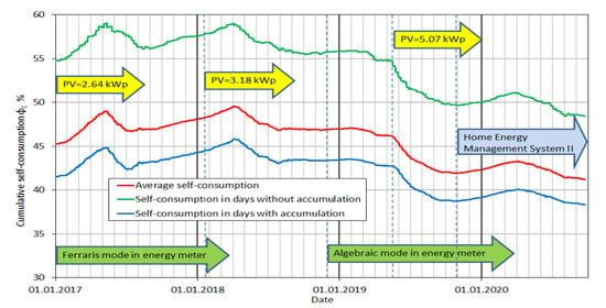
Cumulative year self-consumption charts (Figure 15) were separately prepared for each year. The indicators on the timeline show the PVS build-up moments. The value of the self-consumption at the end of the year corresponds to its average annual value. A visible drop in value for each subsequent year is due to an increase in the PV power, and is indicated in publications [12,13].

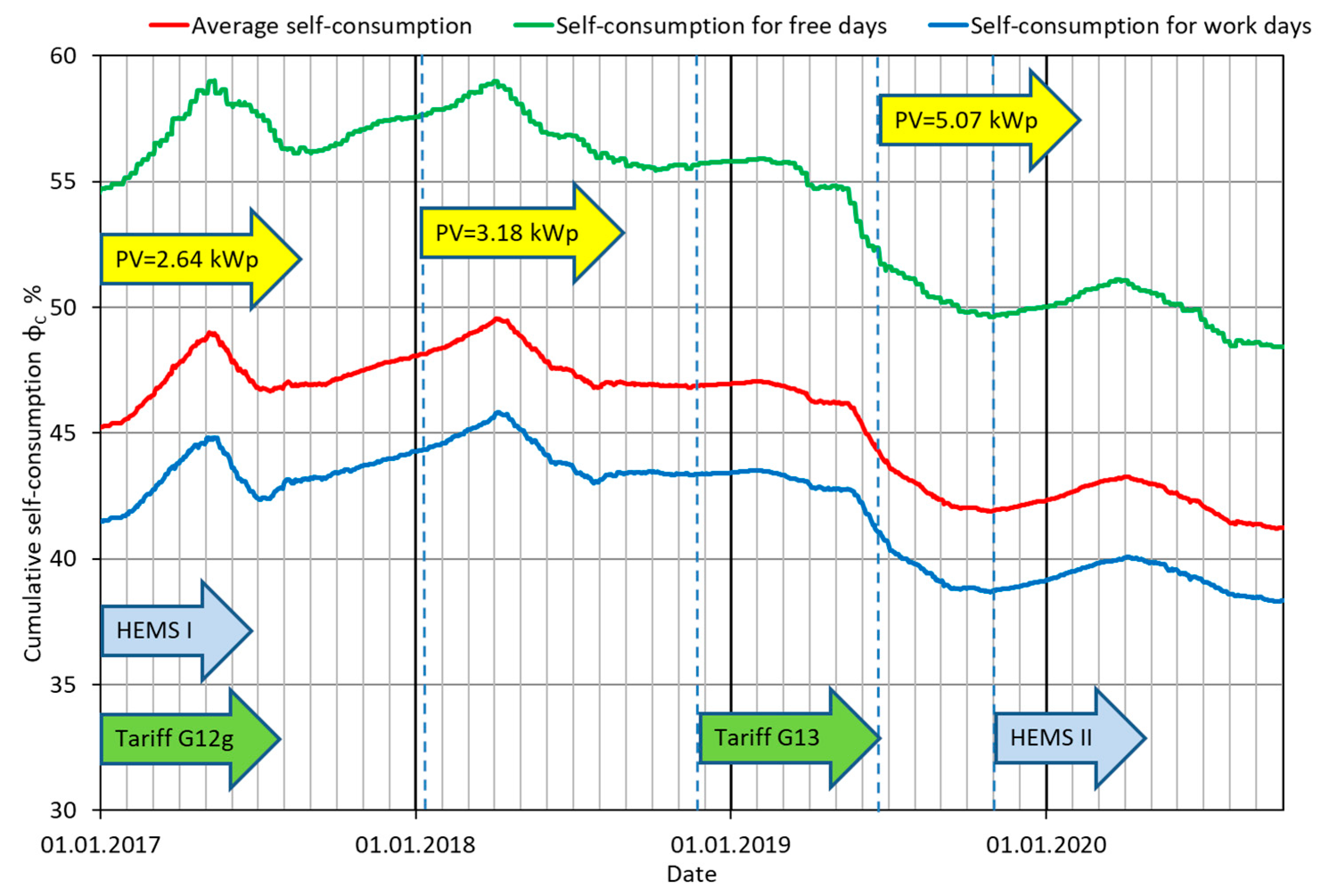
Figure 16 shows the cumulative relative energy consumption since the beginning of the PVS operation; it shows even better all the changes that were made. It also shows the cumulative self-consumption on free and work days. In 2019, it points out the lack of increase in self-consumption in the first 3-4 months of the year (due to a different algorithm in the energy meter), and its sudden drop after the installation of additional PV power. In October of 2019, the new version of HEMS was introduced to increase the self-consumption, which increase is shown in Figure 15 and Figure 16.

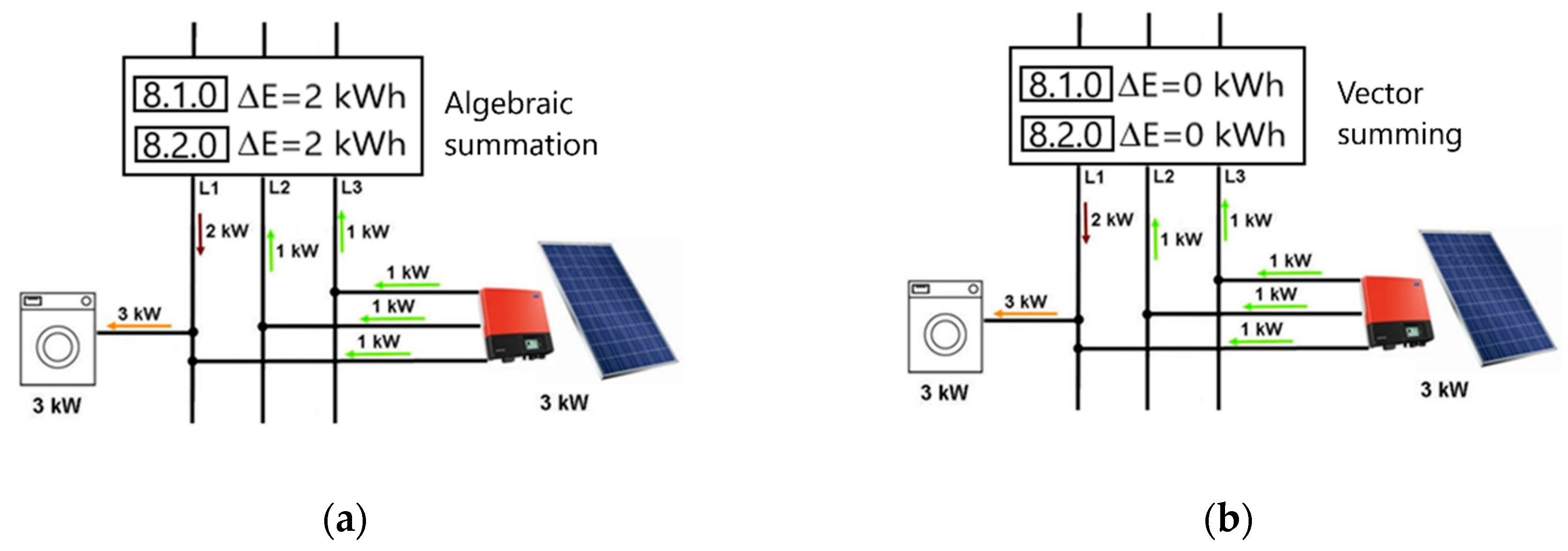
The new function allows for the control of the direction of energy flow on each phase, and switches the loads between phases so as to prevent simultaneous energy flow in both directions. Thanks to this, as long as there is enough energy from the PVS to power all the equipment in the building, it is not taken from the grid. As a result of use of the HEMS, the self-consumption here is greater than in 2019, although the energy meter still operates in the algebraic summation mode. The new operation of the HEMS will not be presented in this article, but only mentioned, pointing to its potential to increase self-consumption.

Table 6. Calculation parameter for year period.

		All Days	Work Days	Free Days
COPavg	-	3.14	2.88	3.80
Tavg	°C	10.4	10.2	11.0
Self-consumption	%	34.7	31.7	41.2

presents the calculated average COP values, average temperature and average self-consumption for the whole year, split into work and free days.

Table 7. Calculation parameter for season period.

		Heating Season			Summer Season
		All Days	Work Days	Free Days	All Days	Work Days	Free Days
COPavg	-	3.23	3.13	3.49	2.97	2.91	3.05
Tavg	°C	6.4	6.4	6.4	19.8	19.8	19.5
Self-consumption	%	46.3	42.2	55.7	31.8	29.0	37.7

also presents the same parameters calculated separately for both seasons. In the analyzed year, the average COP was 3.14 and the average outdoor temperature was 10.4 °C. These values can be considered representative, although the average 10-year outdoor temperature for this location is 10.0 °C, whereas it has already been 10.6 °C for the last 5 years [28].

During the heating season, heat is mainly generated for heating needs, and although the outdoor temperatures are lower, the average COP reaches lower values in summer (COP = 2.97) than in winter (COP = 3.23), at the average annual COP = 3.14. In case of the AWHP, it is normal that the average COP in the summer is lower than in the heating season.

The calculated COPs are higher without heat accumulation in the heating season by 11.5% and in the summer only by 4.8%. These are significant differences, but the economic benefits of using heat storage leave no doubt as to its purpose.

Generally, heat accumulation lowers COP and self-consumption, and this increases energy consumption, but shifts the load into a zone of cheaper energy pricing. In annual terms, self-consumption is on average higher by 9.5%, being 8.7% higher in the summer and 13.5% higher in the heating season. The average annual self-consumption ratio on free days is 41.2%, while in the heating season it is 55.7%, and it is 37.7% in the summer season. The energy management in the building was adjusted to minimize the building’s operating costs, rather than to maximize its self-consumption energy from the PVS.

5.2. The Economic Effects of Heat Storage

Several indicators can be used to assess the profitability of investments, considering inflation and rising energy costs. To simplify considerations, the heat accumulation costs are included as amortization, which is added to the current costs during the lifetime.

Table 8. Energy exported, imported, and consumed in the building.

Tarif	Year	Energy
		Energy Import	Energy Export	PV Generation	PV Self-Consumption		Consumption	PV Self-Sufficient
		kWh	kWh	kWh	kWh	%	kWh	%
G13	2019	7170	2205	3290	1143	34.7	8313	35.0
G12g	2018	7523	1217	2204	987	44.8	8510	23.0
G12g	2017	7810	879	1727	873	50.5	8683	18.2

shows the annual energy quantities exported, imported, and generated from the PV, including the energy used in the building over the 3 years. In addition to the self-consumption ratio, the self-sufficient ratio is also given. This is defined as the sum of the self-consumption of energy from the PV and the energy recovered as a rebate relative to the energy consumed in the building. In 2019, it was 35%. Based on the data from Table 8, and the energy costs (as decided by the President of the Energy Regulatory Office [29]) given in

Table 9. Cost of energy in selected tariffs in Poland in 2019.

Tariff	G11	G12g	G13
Price	EUR/kWh
Zone T1	0.1305	0.1624	0.1163
Zone T2		0.0713	0.1847
Zone T3			0.0622

for the analyzed tariffs, the cost of energy use in the building was calculated, and is presented in

Table 10. Cost of energy exported, imported, and consumed in the building under the G13 and G12g tariffs.

Tariff	Year	Cost
		Import	Export	PV Generation	Consumption	Import-Rebate	Energy Saving
		EUR	EUR	EUR	EUR	EUR	EUR	%
G13	2019	527	162	242	611	397	214	35.0
G12g	2018	665	108	195	753	579	173	23.0
G12g	2017	697	79	154	775	635	141	18.2

.

The question that arises is whether it is worth using multi-zone tariffs in Poland. If the energy from PV meets the annual needs, the choice of tariff is determined by fixed energy costs. If this is not the case, then the choice of tariff is important.

At the beginning, the costs were calculated if only the tariff was changed to G11, but without changing the control of the HS. The results are shown in

Table 11. Cost of energy exported, imported, and consumed in the building directly, recalculated simply to G11 tariff.

Tariff	Year	Cost
		Import	Export	PV Generation	Consumption	Import-Rebate	More Than in Tariff G12g G13
		EUR	EUR	EUR	EUR	EUR	EUR	%
G11	2019	897	250	429	1046	698	301	75.7
G11	2018	981	159	288	1110	854	275	47.5
G11	2017	1019	115	225	1133	927	293	46.1

. The savings with multi-zone tariffs G12g and G13 increase with the power of the PV installations. They would reach 75% in 2019.

However, the accumulation is not necessary when using a single-zone tariff. As shown earlier, heat accumulation lowers the COP HP and reduces the self-consumption of energy from the PV. So is it worth investing in heat accumulators and choosing a multi-zone tariff? To determine this, calculations were made. It was assumed that if the G11 tariff was used, the self-consumption and COP would be the same as in the days without heat accumulation.

The calculations were made for 2019 only, because the analysis showed that only in that year were the export and import of energy on the days with and without accumulation similar (see Table 1 and Table 2).

In the first step, the amount of energy consumed was calculated, taking into account the change in COP and $k_{warm}\left(S_i\right)$—the share of energy consumed by the PC for heat generation for the needs of heating and DHW. The calculations were made separately for both seasons, $S_i$, and for each of the time zones, $T_i$, of the tariff G13.

$$E_{G11cons}\left(S_i, T_i\right)=E_{G13cons}\left(S_i, T_i\right)\left(k_{warm}\left(S_i\right)\frac{CO{P}_{workdays}\left(S_i\right)}{CO{P}_{freedays}\left(S_i\right)}+\left(1-k_{warm}\left(S_i\right)\right)\right)$$

(3)

In the second stage, the amount of imported energy was corrected due to the fact that the self-consumption rate is higher given unnecessary heat accumulation. To calculate energy exported, $E_{PV}\left(S_i,T_i\right)$, in each of the tariff time zones, $T_i$, of the G13 tariff, the energy generated from the PV in these zones was first calculated using Equation (4):

$$E_{PV}\left(S_i,T_i\right)=\frac{E_{G13export}\left(S_i,T_i\right)}{\left(1-{\mathsf{\Phi }}_{workdays}\left(S_i\right)\right)}$$

(4)

Then, formula (5) calculated the energy exported if tariff G11 was used, assuming the self-consumption ratio for free days, ${\mathsf{\Phi }}_{freedays}$.

$$E_{G11export}\left(S_i,T_i\right)=E_{PV}\left(S_i,T_i\right)\left(1-{\mathsf{\Phi }}_{daysoff}\left(S_i\right)\right)$$

(5)

In the last step, imported energy was calculated according to Equation (6).

$$E_{G11import}\left(S_i,T_i\right)=E_{G11cons}\left(S_i,T_i\right)-E_{G11export}\left(S_i,T_i\right)$$

(6)

The sum of energy for each period was calculated, and their comparison with the measurements for the G13 tariff are shown in

Table 12. Recalculation of energy consumption from tariff G13 to tariff G11 in 2019.

Tariff	Energy
	Import	Export	PV Generation	PV Self-Consumption		Consumption	PV Self-Sufficient
	kWh	kWh	kWh	kWh	%	kWh	%
G13	7170	2205	3290	1143	35	8313	35.0
G11	6046	1950	3290	1340	41	7996	36.3

.

As expected, the amount of energy consumed would be lower if the G11 tariff was used. However, this small increase in energy consumption (by 317 kWh) cannot compensate for the cost of energy (

Table 13. Cost of energy exported, imported, and consumed in the building, recalculated to the G11 tariff.

Tariff	Cost
	Import	Export	PV Generation	Consumption	Import-Rebate	Savings	More Than in G13 Tariff with PV (Without PV)
	EUR	EUR	EUR	EUR	EUR	EUR	EUR	%
G13	527	162	242	611	397	214	188	47
G11	789	254	429	1043	585	458	(433)	(71)

), which was much lower in the G13 tariff.

The building maintenance costs would be 47% higher if the G11 tariff was used. The calculated energy costs would be 71% higher if there was no PV installation. The decision to invest in the HB and the larger DHWB, made many years ago, was positively verified.

5.3. Comparison of Achieved Self-Consumption with other Results

The obtained self-consumption results were compared with the results presented in the article [12] based on data from many buildings. In this article, changes in the self-consumption coefficient for buildings without electric heating (6 kW) and with electric heating (14.5 kW) were determined. Against this background, the results obtained from the analyzed building, for which the maximum power did not exceed 8 kW, are given. The data used were from three cases:

(a)

Determined for the operated state with heat;

(b)

Calculated for the situation wherein there would be no heat accumulation;

(c)

Calculated for same the situation as in point (b), but only for the heating season.

Although the heat accumulation reduces self-consumption, the ratios obtained are slightly better than those presented in the studies. Figure 17 shows the relationship between relative self-consumption and the installed PV’s power.

Figure 18 shows the changes in self-consumption caused by load shift. The self-consumption achieved in the last year is almost the same as that for buildings without load shifts. It is worth noting that without the heat storage, self-consumption was 6% higher, and if considering only the heating season, it was 19% higher in relation to buildings with a load shift.

6. Summary and Conclusions

The increasing generation from the PV, especially in suburban areas, raises increasingly frequent problems, such as switching off the PV due to overvoltage. Such incidents were observed many times in the PVS of the studied building. This problem is growing in Poland, because over the last two years the capacity of prosumer PV generation has doubled annually. Currently, DSOs have no control over the installations up to 10 kWp. One way to absorb large amounts of energy is through the use of HPs. These can significantly increase the stability of the grid if the DSOs provide the DSR. Another solution that could be implemented is energy storage. From the point of view of use, the EESS is the more favorable form. As shown, the heat storage is a cheaper alternative, but its potential in summer is limited. However, the generation of cold with HPs has great potential.

This article discusses the impact of heat accumulation on COP and self-consumption. It was shown that accumulation can significantly reduce energy bills through a shift load and a multi-zone tariff, as can the DSM instrument. In the analyzed building, for which the self-sufficiency ratio was 35%, the savings were over 40%. For the same building without PV, load shift and energy storage, the cost of energy would be over 70% higher. The heat storage had a negative impact on PV energy self-consumption, reducing it from 41% to 35%.

There are other ways of increasing self-consumption, for example through the HEMS, with the aim of reducing energy imports. The internet of thigs (IoT) could be useful if the momentary electric power of the devices could be controlled. The authors are developing this direction of increasing self-consumption. Currently, the IoT only lets the home-users switch devices on and off.

References

1. Schibuola, L.; Scarpa, M.; Tambani, C. Demand response management by means of heat pumps controlledvia real time pricing. Energy Build. 2015, 90, 15–28. [Google Scholar] [CrossRef]
2. Polish Power Grids-DSR Programs. Available online: https://dsr.pse.pl/ (accessed on 15 January 2020).
3. Hoppmann, J.; Volland, J.; Schmidt, T.S.; Hoffmann, V.H. The economic viability of battery storage for residential solarv photovoltaic systems—A review and a simulation model. Renew. Sustain. Energy Rev. 2014, 39, 1101–1118. [Google Scholar] [CrossRef]
4. Castillo-Cagigal, M.; Caamaño-Martín, E.; Gutiérrez, A.; Masa-Bote, D.; Monasterio, F.; Porro, J.; Matallanas, E.; Jiménez-Leube, J. Self-Consumption of PV Electricity with Active Demand Side Management: The GeDELOS-PV System. In Proceedings of the 25th European Photovoltaic Solar Energy Conference and Exhibition/5th World Conference on Photovoltaic Energy Conversion, Valencia, Spain, 6–10 September 2010. [Google Scholar]
5. European Comission. Local Storage: The Way Forward for Solar PV? Strategic Energy Technologies Information System; Publications Office of the European Union: Luxembourg, 2013. [Google Scholar]
6. Steel, W. Sweden set to launch residential energy storage scheme. Renew Energy World 2016, 23. Available online: https://www.renewableenergyworld.com/2016/10/26/sweden-set-to-launch-residential-energy-storage-scheme/html (accessed on 20 March 2020).
7. EN-50438 Requirements for Micro-Generating Plants to Be Connected in Parallel with Public Low-Voltage Distribution Networks; European Committee for Electrotechnical Standardization: Brussels, Belgium, 2015.
8. IEC 61000-3-3. Electromagnetic Compatibility (EMC)—Part 3-3: Limits—Limitation of Voltage Changes, Voltage Fluctuations and Flicker in Public Low-Voltage Supply Systems, for Equipment with Rated Current ≤16 A per Phase and not Subject to Conditional Connection; European Committee for Electrotechnical Standardization: Brussels, Belgium, 2013. [Google Scholar]
9. IEC 61000-3-11. Electromagnetic Compatibility (EMC)—Part 3-11: Limits—Limitation of Voltage Changes, Voltage Fluctuations and Flicker in Public Low-Voltage Supply Systems—Equipment with Rated Current ≤75 A and Subject to Conditional Connection; European Committee for Electrotechnical Standardization: Brussels, Belgium, 2019. [Google Scholar]
10. Ustawa z dnia 20 lutego 2015 r. o odnawialnych źródłach energii. Dziennik Ustaw 2015, 478.
11. Wyrsch, W.; Riesen, Y.; Tschui, R.; Boillat, C.; Ballif, C. Demand Side Management for Enhanced Integration of Photovoltaics into Grid. In Proceedings of the 31st European Photovoltaic Solar Energy Conference, Hamburg, Germany, 14–18 September 2015. [Google Scholar] [CrossRef]
12. Widén, J. Improved photovoltaic self-consumption with appliance scheduling in 200 single-family buildings. Appl. Energy 2014, 126, 199–212. [Google Scholar] [CrossRef]
13. Luthander, R.; Widén, J.; Nilsson, D.; Palm, J. Photovoltaic self-consumption in buildings: A review. Appl. Energy 2015, 142, 80–94. [Google Scholar] [CrossRef] [Green Version]
14. Williams, C.J.C.; Binder, J.O.; Kelm, T. Demand Side Management through Heat Pumps, Thermal Storage and Battery Storage to Increase Local Selfconsumption and Grid Compatibility of PV Systems. In Proceedings of the 3rd IEEE PESinternational conference and exhibition on innovative smart grid technologies (ISGT Europe), Berlin, Germany, 14–17 October 2012; pp. 1–6. [Google Scholar]
15. Thygesen, R.; Karlsson, B. Simulation and analysis of a solar assisted heat pump system with two different storage types for high levels of PV electricity selfconsumption. Sol. Energy 2014, 103, 19–27. [Google Scholar] [CrossRef]
16. Omaji, S.; Javaid, S.; Javaid, N.; Syed, H.A.; Muhammad, K.A.; Ishmanov, F. An Efficient Power Scheduling in Smart Homes Using Jaya Based Optimization with Time-of-Use and Critical Peak Pricing Schemes. Energies 2018, 11, 3155. [Google Scholar] [CrossRef] [Green Version]
17. Ahmed, M.S.; Mohamed, A.; Khatib, T.; Shareef, H. Real time optimal schedule controller for home energy management system using new binary backtracking search algorithm. Energy Build. 2017, 38, 215–227. [Google Scholar] [CrossRef]
18. Campoccia, A.; Dusonchet, L.; Telaretti, E.; Zizzo, G. An analysis of feed’in tariffs for solar PV in six representative countries of the European Union. Sol. Energy 2014, 107, 530–542. [Google Scholar] [CrossRef]
19. Legal Sources on Renewable Energy—Compare Support Schemes. Available online: http://www.res-legal.eu/compare-support-schemes (accessed on 12 January 2020).
20. Best Practices on Renewable Energy Self-Consumption. In Commission Staff Working Document; EU Commission: Brussels, Belgium, 2015.
21. Ustawa z dnia 29 grudnia 2015 r. o zmianie ustawy o odnawialnych źródłach energii oraz ustawy—Prawo energetyczne. Dziennik Ustaw 2015, 2365.
22. Briano, J.I.; Baez, M.J. A Methodology for the Analysis of PV Self-Consumption Policies. Report IEA-PVPS T1-28. 2016. Available online: https://iea-pvps.org/wp-content/uploads/2020/01/IEA-PVPS_-_A_methodology_for_the_Analysis_of_PV_Self-Consumption_Policies.pdf (accessed on 11 April 2020).
23. Viessmann. Product Literature, Drawings, Images and other Resources Available for Download. Available online: https://www.viessmann-us.com/en/services/downloads.html (accessed on 21 January 2020).
24. Price List 2011 PL; Publ. Viessmann Sp. z o.o.: Wrocław, Poland, 2011.
25. Available online: https://www.solarchoice.net.au/is-home-battery-storage-worth-it/ (accessed on 9 September 2020).
26. Velik, R. East-West Orientation of PV Systems and Neighbourhood Energy Exchange to Maximize Local Photovoltaics Energy Consumption. Int. J. Renew. Energy Res. 2014, 4, 566–570. Available online: https://www.ijrer.org/ijrer/index.php/ijrer/article/view/1293 (accessed on 10 August 2020).
27. Mubarak, R.; Luiz, E.W.; Seckmeyer, G. Why PV Modules Should Preferably No Longer Be Oriented to the South in the Near Future. Energies 2019, 12, 4528. [Google Scholar] [CrossRef] [Green Version]
28. Typical Meteorological Years and Statistical Climate Data for the Area of Poland for Energy Calculations of Buildings. Available online: https://dane.gov.pl/dataset/797,typowe-lata-meteorologiczne-i-statystyczne-dane-klimatyczne-dla-obszaru-polski-do-obliczen-energetycznych-budynkow (accessed on 20 December 2019).
29. Biuletyn Informacji Publicznej, Urząd Regulacji Energetyki. Available online: https://bip.ure.gov.pl/bip/taryfy-i-inne-decyzje-b/energia-elektryczna (accessed on 10 December 2019).
Figure 1. The diagram illustrates the rebate system for prosumers in Poland.
Energies 13 05476 g001
Figure 2. Differences in registers of three-phase energy meters for mode: (a) algebraic summation, (b) vector summation for an example generation and a load.
Energies 13 05476 g002
Figure 3. Graphs of generation, consumption and export of energy on 18 March 2019 for a meter with (a) arithmetic (b) vector mode.
Energies 13 05476 g003
Figure 4. The existing HS diagram in the test building. Main components: HP Vitocal 200S, HB 1 Vitocell 100-V 400 dm3, HB 2 Vitocell 100-E 200 dm3, DHWB Vitocell 100-V 390 dm3.
Energies 13 05476 g004
Figure 5. An example of daily PVS generation on 24th May 2019.
Energies 13 05476 g005
Figure 6. Possibilities of energy accumulation in the HBs and the DHWB.
Energies 13 05476 g006
Figure 7. Time schedule for heat accumulation in the HBs and the DHWB on work days.
Energies 13 05476 g007
Figure 8. Temperatures in the HB 2 and circuits, and HP state, on work days.
Energies 13 05476 g008
Figure 9. Over three years of data collection of energy import and export.
Energies 13 05476 g009
Figure 10. Over three years of data collection of energy PV generation, PV self-consumption and HP consumption.
Energies 13 05476 g010
Figure 11. Structure of energy use in months in the building.
Energies 13 05476 g011
Figure 12. Seasonal dependencies of COP for work days and free days.
Energies 13 05476 g012
Figure 13. Relative self-consumption as a function of the daily PV generation, indicating the months of the year.
Energies 13 05476 g013
Figure 14. Relative self-consumption as a function of daily generation with PV divided into work and free days.
Energies 13 05476 g014
Figure 15. Cumulative self-consumption average in a period of one year for the 3 next years.
Energies 13 05476 g015
Figure 16. Cumulative self-consumption from the beginning of PVS’s existence.
Energies 13 05476 g016
Figure 17. Comparison of calculated relative coefficient PV self-consumption to PV size averaged over all 200 households [12].
Energies 13 05476 g017
Figure 18. Comparison of relative self-consumption to average self-consumption, with and without load shifting and for different PV system sizes [12].
Energies 13 05476 g018