Laser Scanner-Based 3D Digitization for the Reflective Shape Measurement of a Parabolic Trough Collector

Abstract

In concentrated solar power technology, the precise shape of the reflective surfaces is crucial for efficiency. Considering the geometry and size of a parabolic trough collector, measuring the actual shape is not trivial and some techniques can only be adopted during the assembly operations, evaluating only the manufacturing and alignment processes. The method proposed and tested in this work exploits a laser scanner-based three-dimensional digitization technique that can be used without any marker or other tools, and is attached to the structure. This technique is particularly suitable for assessing the behavior and the optical efficiency of the collectors under load and for validating a finite element model of the structure. The method defines the shape of the parabolic surface by collecting a 3D point cloud of the parabolic surface using a laser scanner. The measured form can then be compared with the ideal shape obtained from a finite element analysis of the structure subject to the gravity field. The comparison can also be performed when the collector is loaded by known forces or torques, with the finite element model reproducing the actual loading scenario. The object of the case study of this work was a 12 m wide full-scale prototype trough collector manufactured at the Politecnico di Milano. The uncertainty of the 3D measurements, acquiring twelve images in different positions, was verified to be less than 3.6 mm.

1. Introduction

Parabolic trough collectors represent the most popular layout used in concentrated solar power (CSP) systems. The main characteristic of CSP systems, which has drawn the attention of many investors and countries, is the possibility to heat up and accumulate a working fluid in a storage system. Even though solar irradiation is not available 24 h/day, CSP systems can generate electrical energy for the base load of the electrical demand comparable to thermal power plants based on fossil fuel. This feature represents a promising advantage among other renewable energy technologies [1,2].

Parabolic trough collectors are made of reflective panels or mirrors able to reflect and concentrate the sunlight onto a receiver tube, located in the focus zone of the parabola, where a gas or a mixture of molten salts is heated up and combined in a thermodynamic cycle. Evaluating the actual parabolic shape of the collectors is necessary to guarantee the expected efficiency of the installed system or, in the prototype phase, to improve the assembly procedures for large-scale production. The precise shape of the reflective surfaces is crucial for optical efficiency which, in turn, affects the overall efficiency of the installed systems.

Different optical measurement techniques, based on the precision requirements needed, have been used over the past three decades for geometrical assessment and optimization of solar collectors. Some of these methods include photogrammetry [3,4,5], the video scanning Hartmann optical test (VSHOT) [6] and deflectometry [7].

The methods based on photogrammetry focus on specific points identified by targets that need to be installed on the solar trough at the manufacturing stage, maintaining enough positional accuracy. Such physical addition to an already sophisticated mechanical device would involve a traceable metrological chain for guaranteeing that the relative position of the targets to the body of the solar trough is known within an assigned tolerance at the mounting stage. This adds a further layer of manufacturing complexity (and costs). Furthermore, a preliminary survey for characterizing the target-to-structure relative positioning is needed, before the actual measurement of the targets when the reflector is in operating conditions. Another limitation of the photogrammetric approach is that only a few measured 3D points are involved in quality control. Therefore, no high-resolution surface analysis is possible and any measurement error on the few measured points heavily affects the result having each point a higher weight in the shape evaluation of the reflecting surface.

The video Hartman optical tester (VSHOT) is a dedicated slope-measuring tool for large reflectors. It consists of a square planar target with a little aperture in the center, from which a laser source generates a beam orthogonal to the target plane. The laser-target ensemble is positioned in front of the specimen reflector at a distance slightly greater than twice its focal length. With its axis almost orthogonal to the target plane, a camera aiming at the target records the laser spot back-reflected over the target by the specimen reflector. By analyzing the position of such spot over the target, given the target-to-mirror distance, it is possible to estimate the reflector’s local slope in the point illuminated by the laser beam. For this reason, the laser-target system is controlled by a 2-axis scanner for exploring a predefined area of the specimen reflector. By mapping an entire area of the reflector, its closeness to a parabolic shape is determined.

This method has the advantage of high accuracy. The repeatability reported was 0.02%, with a bias error of 0.24% and a standard deviation of 0.45% [8]. On the other hand, this is a cumbersome custom system, needing calibration before each use, and not easily portable. The factors mentioned above make such a method more suitable for a manufacturer in a custom facility than for taking measurements on the field in operating conditions.

Deflectometry is a similar technique where, instead of a single laser beam, sinusoidal fringe patterns generated by an LCD projector are projected onto the reflector under test. A screen located in front of the solar trough allows observing the fringe patterns reflected from the surface. Any slope variations of the surface lead to distortions of the patterns. Such distortions are measured by comparing them to the reflections expected by mathematical simulation of the ideal surface [9]. Compared to the VSHOT method, the measuring time is much shorter, thanks to the absence of any mechanical scanning, therefore the system is suitable also for checking at high resolution large solar reflectors [10]. The measurement accuracy is high as in VSHOT, but also this method is based on a custom prototype requiring a complex calibration before each measurement.

Great precision is required while assessing a new design [11], whereas speed and cost are the most important factors when characterizing entire solar fields already in operation [12]. A comparative study analyzing the time needed for the data collection demonstrated the advantages of laser scanning over photogrammetry. Scans of the reflective surfaces of collectors are generally not possible, whereas scans of the rear side of the collector provide an opaque surface which makes the geometric assessment and optimization possible, provided that the point density is high and the accuracy requirements are lower than those required for the assembly stage verification [13].

In this work, an alternative evaluation method for estimating the actual shape of a parabolic trough collector is proposed and tested. It consists of collecting a 3D point cloud of the parabolic surface using a laser scanner and comparing the measured shape with the ideal shape obtained from a finite element analysis (FEA) study of the collector. In this case, both the experimentally measured and the simulated structure are only loaded by gravity. The 3D scanned data are processed to reduce noise before the comparison. This procedure aims to verify the quality of the manufacturing process of the parabolic trough collector.

The advantages of the proposed method over the preexisting methods are multiple. First, it is not based on cumbersome custom devices to be installed in front of the solar trough for its quality check like with VSHOT and deflectometry; it uses instead an off-the shelf device for general purpose reverse engineering. Secondarily the device used is light and portable so that the same approach can be easily transferred from a lab in a manufacturing site to the field in operating conditions. Third, it does not need the use of any custom target embedded in or attached to the reflector like with photogrammetry, getting rid of any customization finalized to quality control. Fourth, by using the rear side of the reflector as opaque measuring surface, some issues associated with the difficult access to the frontal part of the reflector during certain orientations (i.e., with the concavity pointing to the sky) are eliminated. In [11] for example the need of an hydraulic platform for taking the images from above the reflector is documented. In our case the solar trough in the same orientation is digitized from behind, with the scanning unit on the ground.

This method can furthermore be used when known loads are applied to the structure. The comparison between experimental measurement and FEA results can be performed, provided that all the loads can be correctly simulated in the FE model. In this case, the method can be useful for validating the FE model or evaluating the behavior of the structure, in terms of displacements and optical performances when the system is operational, or when it is submitted to unplanned circumstances. Measurements were taken with gravity only or with the structure loaded by torsion, a typical operational load of this system, as collectors must be continuously rotated to reach perpendicular sunlight during the daylight hours.

The collector studied in this work was a 12 m wide full-scale parabolic trough collector prototype manufactured in the laboratory of the Department of Mechanical Engineering of the Politecnico di Milano and developed in cooperation with the Italian energy company Eni and the Massachusetts Institute of Technology (MIT).

2. Methodology

2.1. 3D Digitization

Examining a physical object by capturing its shape with a three-dimensional (3D) digitizer and comparing it with the corresponding computer-aided design (CAD) model is nowadays a standard quality control process for objects in the order of 1 m in size. For this purpose, 3D technologies based on triangulation can be used. However, when the size of the object to certify is above a certain limit, certifying its shape with small tolerances can be difficult.

3D digitization is a widely used process to measure a physical object by creating digital data in the form of a 3D point cloud representing a sampling of the object’s surface. This data is used to measure and determine the shape of an object in a fast and accurate manner, which can be used for several engineering applications such as reverse engineering [14,15], rapid prototyping [16], and quality control [17]. 3D digitization in industrial applications can be obtained employing different active methods, involving either laser scanning or pattern projection, or through passive techniques such as photogrammetry.

3D digitization is increasingly present in quality assurance systems. For metrological quality inspection purposes, 3D data is collected from physical objects and compared with their theoretical digital models. Even though the accuracy of the measured data acquired by 3D devices is intrinsically lower than the data acquired by high-level coordinate measuring machines (CMMs), several tests have proven that optical 3D digitization can be successfully used in complex geometrical inspections that meet currently defined accuracy demands. 3D digitization can provide accurate measurements by using a high-end system, reducing the noise by fitting the best shape according to the feature (such as a plane, a cylinder or a sphere) to the acquired point cloud [18,19]. Moreover, 3D acquisition is often used for workpiece inspection, deformation analysis, and reverse engineering of molds and dyes for the automotive industry [20], aerospace industry [21], consumer and medical product design [19,22], and general quality control procedures [23].

2.2. Data Acquisition and Comparison Strategy

The quality check of this work was carried out by reverse engineering the physical structure with a 3D laser scanner [24]. This process generated a reality-based dense 3D point cloud from the rear side of the collector for each condition considered, containing a high-resolution spatial representation of the actual shape deformations. This 3D cloud was then compared to the theoretical shape of the same object represented by a 3D model, evaluating systematic deviations within the measurement uncertainty of the laser tool employed in this test, according to the procedure described in the next section, “test procedure.”

The deviation was therefore measured in two operating conditions: (a) without any externally applied stress (only gravity load) applied to the structure; (b) with a torsion applied at the ends of the collector. Correspondingly, the 3D point cloud obtained by 3D scanning was compared with: (a) the numerical model of the structure, as conceived in the design phase, taking into account the effects of gravity through FEA; (b) the simulation of the structure distortion obtained by FEA, with the same loading conditions used in the experiments.

Furthermore, the degree of deviation of the parabolic profile of the structure, loaded with gravity only, was tested at different positions over the 12 m width of the collector. The measured point cloud was sampled in different cross-sections along the collector surface to evaluate the actual effect of gravity with the collector in a vertical position (i.e., with the parabola axis parallel to the floor).

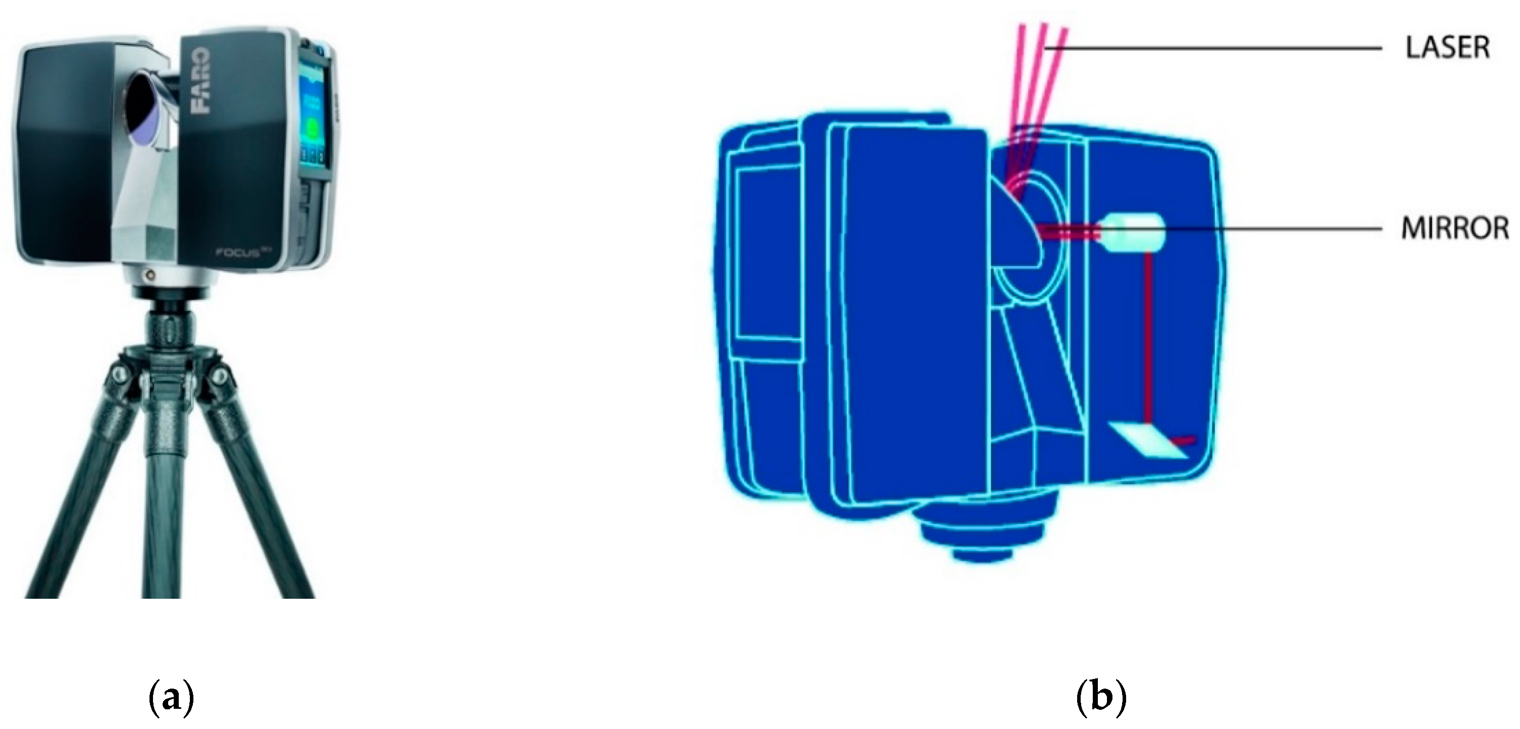
2.3. Features of the 3D Device Used

The instrument employed for measuring the collector geometry was a Focus3D 120S (Figure 1a), a phase-shift laser scanner from the manufacturer Faro (Lake Mary, FL, USA). The Faro Focus3D sends an infrared laser beam to the center of its rotating mirror. The mirror deflects the laser beam on a vertical rotation around the environment to be scanned (Figure 1b) and the scattered light from surrounding objects is then reflected back to the scanner.

In order to measure the distance, the Focus3D uses phase shift technology, which projects constant waves of sinusoidal modulated infrared light with varying wavelength outward from the scanner. Upon contact with an object, the waves are back-reflected to the scanner and compared with the transmitted waves to determine the phase shift, proportional to the scanner-to-target distance.

While the mirror rotates, it generates a circular scanline that in principle covers 360 degrees. After each complete rotation of the mirror, the scanner rotates around the vertical axis of a predefined angular step, which can be as small as 0.009° degrees, and the horizontal and vertical angles are acquired through an encoder. The scanner stops acquiring data when the beam is oriented towards the lower part of the instrument, where the tripod is located (Figure 1a). For this reason, the scanner covers a field of view of 360° degrees horizontally (Figure 2a) and 305° degrees vertically (Figure 2b).

The x, y, z coordinates of each point are then calculated by using angle encoders to measure the mirror rotation and the horizontal rotation of Focus3D. Distance, vertical angle and horizontal angle make up polar coordinates (ρ, α, β), which are then transformed to Cartesian coordinates (x, y, z).

The nominal measurement uncertainty of this device on a 10% reflectance diffusive target located at 25 m from the scanner is 2.2 mm. This data is provided by the manufacturing company through the maximum ranging error of ±2 mm with zero average on repeated measurements, and the ranging noise, evaluated as the standard deviation of error over a fitting plane calculated on the 3D scan of a planar target scanned at 122,000 points/sec (

Table 1. Technical features of the laser scanner used in the experiments from the device’s manual.

Ranging Unit	Unambiguity interval: 153.49 m (503.58ft) Range Focus3DS 120: 0.6 m–120 m indoor or outdoor with low ambient light and normal incidence to a 90% reflective surface Measurement speed (pts/sec): 122,000/244,000/488,000/976,000 Ranging error: ±2 mm at 10 m and 25 m, each at 90% and 10% reflectivity
Ranging noise	@10 m	@10 m—noise compressed	@25 m	@25 m—noise compressed
@90% refl.	0.6 mm	0.3 mm	0.95 mm	0.5 mm
@10% refl.	1.2 mm	0.6 mm	2.20 mm	1.1 mm
Laser (Optical transmission)	Laser power (cw θ): 20 mW (Laser class 3R) Wavelength: 950 nm Beam divergence: Typical 0.19 mrad (0.011°) Beam diameter at exit: Typical 3.0 mm, circular

) [25].

If the surface scanned is, however, not perfectly diffusive, the reduced amount of light reflected to the device decreases the signal to noise ratio during the phase-shift measurement, consequently increasing the measurement uncertainty up to a few times the nominal, as verified experimentally in laboratory tests. Finally, the registration process required for creating a single 3D point cloud from different 3D images taken around the object, involving the minimization of the mean square distance between partially overlapping 3D images, potentially further contributes to uncertainty. Uncertainty on average metallic surfaces, whose behavior is partially specular, at 25 m is expected to be in the range of 2.5 to 10 mm.

3. Test Procedure

3.1. 3D Scanner Measurements

3.1.1. Instrument Placement

Owing to its working principle, a laser scanner does not work on highly reflective surfaces because no light wave is sent back to the instrument sensor, making 3D measurements impossible. Therefore, the rear part of the trough collector surface, which is metallic and only partially specular, whose offset from the actual reflective surface is 1.5 mm, was scanned. The residual specularity, visible only when the laser beam is oriented at right angles, generates limited geometrical artifacts such as those shown in Figure 3.

The only drawback of this approach, in the case of the studied prototype, were several occlusions generated on the rear part of the trough collector by the holding structure made by seven parabolic-shaped transversal ribs along the 12 m width. These ribs prevented the scanning of the rear trough collector area in a single laser scan.

The area was thus scanned in sections for each of the six inter-rib spaces. Two scans for each space were taken, one above and one below the parabola vertex as indicated in Figure 4b, and the total of 12 scans for each one of the two operating conditions were evaluated: (a) loaded by gravity only; (b) with an additional torsional load applied.

The upper set of the scans was taken with the tripod mounted on a 2 m tall scaffolding, holding the laser scanner at approximately 3.6 m above the floor, with the instrument located horizontally in the space between two adjacent transversal ribs at a distance of about 5 m from the rear side of the trough collector. Since the ribs are spaced 2 m apart from each other, the scans were repeated translating the scaffolding horizontally (along the z-axis shown in Figure 4b). In contrast, the lower set of scans was taken with the tripod of the laser scanner located on the ground, holding the instrument at approximately 1.6 m above the floor.

Considering the time needed for each 3D measurement and the repositioning of the instrument in the various positions, the whole procedure took about 1 h. However, in an in-situ automatized process, the total amount of time can be optimized and reduced to a few minutes.

3.1.2. Instrument Settings

Each 3D image was taken with the laser power setting near the minimum to reduce the number of reflection artifacts shown in Figure 3. The actual instrument profile used was “Indoor 10 m” starting from the bottom level, which made it possible to capture not only the rear surface of the trough collector but also the surrounding environment, used as a reference for the subsequent alignment step.

The resolution setting of the Focus3D is defined by selecting the undersampling level with respect to the full resolution, which corresponds to an angular step of 0.009° (0.15 mrad), and which, when projected at a 10 m distance, provides a sampling step of 1.5 mm. The spatial resolution can be varied by merely skipping some of the samples collected automatically by the device, such as one point out of two, one point out of four, etc., obtaining different setting levels selectable by the operator. Correspondingly, the number of 3D samples forming the full spherical scanning is progressively reduced from the initial 711 million points to a more manageable number (see

Table 2. Resolution and 3D cloud size produced by the Faro Focus3D for different sampling size, for the full scanning angular range (H = 360°; V = 305°).

Sampling Size	1:1	1:2	1:4	1:5	1:8
Δθ (degree)	0.009	0.018	0.035	0.044	0.070
Step @10m (mm)	1.53	3.07	6.14	7.67	12.27
Horizontal size (#3D pixels)	40,960	20,480	10,240	8192	5120
Vertical size (#3D pixels)	17351	8676	4338	3470	2169
3D point cloud size (Mpoints)	710.7	177.7	44.4	28.4	11.1

).

In this case study a level of undersampling of 8 (i.e., only 1 point out of 8), corresponding to a 3D sample spacing of 12.3 mm at a 10 m distance from the instrument was chosen. However, the actual scanner-to-surface distance provided by the scanning geometry ranged from 5 to 13 m, with a sampling step ranging consequently from 6 to 16 mm.

The parameter “quality”, corresponding to the number of repeated measurements of the same point that are averaged to provide the final result, was set to 4, which corresponds to a 2-fold improvement of the signal to noise ratio and quadruplicates the scan time for the same given number of collected points.

Finally, in order to avoid the acquisition of points which are not useful for the required model, while at the same time generating easily manageable 3D images in the following processing step, the vertical scan was reduced from the full extent [−62.5°; +90°] to an angular range more focused on the trough collector size [−45°; +45°], while still maintaining a full 360° horizontal scan. This choice, together with the laser power settings mentioned above, made it possible to include part of the environment surrounding the reflector in each 3D scan, which was useful for the subsequent alignment step.

3.2. Post-Processing Analyses

3.2.1. 3D Data Alignment

The twelve 3D images, acquired by locating the scanner as shown in Figure 4b and with the settings described above, were next registered in a single reference system using the standard “iterative closest points” (ICP) algorithm, based on the minimization of the root mean square distance between a 3D scan, used as reference, and a 3D scan to be registered on the first one.

After a first alignment attempt with the well-known software package Cyclone by Leica Geosystems [26] the residual errors were greater than 10 mm. However, the application of a mild low-pass filtering to the raw 3D data resulted in a significant reduction. In terms of spatial frequency, the noise pattern is in fact characterized by a large bandwidth, covering up to the maximum value associated with the spatial sampling (i.e., 1/sampling step). On the other hand, the structure under measurement is a smoothly changing parabolic surface, which in terms of spatial frequency resides in the lower part of the spectrum.

Therefore, the influence of the random measurement errors (i.e., the large bandwidth noise) was lowered by filtering out the high spatial frequencies, while the tested shape remained unchanged. The “IMAlign” module of the software package Polyworks^® [27], was used for this purpose. This module, in addition to the filtering mentioned above, generates a pre-meshing of point clouds, allowing the implementation of more precise evaluations of the root mean square distance between different 3D scans. The results are demonstrated with the help of error histograms for each 3D scan with respect to all the others, providing powerful feedback for controlling the whole alignment process. In Figure 5, the output of the data alignment operated on the first data set, which was gathered with the trough collector without the application of any load but the gravity load, demonstrates the excellent quality of this processing solution.

The alignment with a substantial data overlap, as performed in this case, also provides a very clear a-posteriori indication of the 3D data uncertainty, which is much more reliable than the information provided by the datasheets of the manufacturer. This improved the uncertainty estimation resulted from the actual measurement condition with the actual material, independently of the assumptions about reflectivity and diffusivity of the target object. Two largely overlapping scans represent the 3D acquisition of the same object with the superposition of different noise instances owing to the actual 3D measurement uncertainty. Once aligned, the analysis of the statistical deviation of one from the other in the overlapping zones made it possible to ignore the component of the shape, which is identical in each of the two scans, considering the random component of the measurement only.

Such a component, if no other systematic source of error occurs, arises from the thermal noise affecting the phase detection electronics, which is well known to be White (i.e., uniformly distributed in the frequency domain) and Gaussian. Therefore, the presence of a Gaussian distribution of random errors shown in the error histograms in Figure 5a allowed the exclusion of an additional systematic source of error such as those associated with residual misalignments of the 3D scans.

This conclusion is further confirmed by the data shown in

Table 3. Residual alignment errors of each range scan as reported graphically in Figure 5. Each range scan is numbered from 1 to 12, and the values are given in mm with respect to scan 2, used as reference and, therefore, omitted from the list.

Scan	Mean (mm)	σ (mm)
1	−0.029	2.98
3	−0.034	2.97
4	−0.027	3.02
5	−0.015	3.08
6	−0.025	3.17
7	−0.037	3.01
8	−0.047	2.90
9	−0.025	3.02
10	−0.002	2.95
11	−0.099	3.01
12	−0.011	2.95

. The table shows residual alignment errors of each range scan, numbered from 1 to 12, with respect to scan 2, used as a reference and therefore omitted from in the list. In Table 3 the geometrical values are represented in mm, in contrast to the values produced by the post-processing software, which presents them in meters, the measurement unit of the laser scanner. These numbers show a residual mean deviation of each re-oriented scan from the reference which was very close to zero (the maximum value in the column “Mean” is 99 micrometers), while the standard deviation of error ranges from 2.90 to 3.17 mm. Such a value is slightly larger than the nominal instrument error, which is coherent with the fact that the scanned surface is not made of a purely diffusive material.

In other words, the analysis of the feedback provided by this process leads to the conclusion that the 3D data alignment is coherent with the instrument tolerance, considering the reduced reflectivity of the scanned material.

In addition, this analysis determines the actual measurement uncertainty (analyzed from the standard deviation of the error reported in Table 3) provided by this process that appears to be lower than 3.2 mm. This means that, with the exclusion of reflections and other recognizable reflection artifacts possibly affecting the specific part of the structure, any deviation from the theoretical shape above 3σ (9.6 mm) is a real deformation of the shape with a confidence level of 99.7%.

As the final step, all the aligned data were merged into a single cloud of nearly 9 × 10⁶ 3D points, representing the 3D image of the actual object, suitable to be compared with a reference model.

3.2.2. Finite Element Analyses

The Finite Element (FE) model of the parabolic trough collector was built using the commercial software Pre/Post Abaqus™ CAE 2016 and the results were computed using the Abaqus™ Standard solver. Figure 6 and Figure 7 show some details of the FE model. The main structure is composed of rows of panels and the posterior reinforcement is made of parabolic ribs, braces and beams.

Many interactions were created to assemble the parts of the structure in a realistic way, including the opportunity to reproduce preloads. In order to reproduce the behavior of the structure, constraints and loads were applied to the model. The gravitational field was always imposed and directed along the negative y-axis. In the case of the applied torsional load, as schematized in Figure 6, one lateral end of the structure was fixed, whereas a torque was applied in the opposite end. This represents a typical scenario of: (i) an unbalanced wind pressure to the whole line of parabolic trough collectors; (ii) an erroneous differential rotation imposed by the actuation system; (iii) another possible obstacle to the rotation. The magnitude of the imposed torque to the prototype was chosen in favor of safety, higher than that expected in a solar field.

With regards to the other boundary conditions, the real prototype was constrained to the ground by means of two bearings on each side, placed on two pylons. In the present model, three bearings were considered as hinges and one hinge as a slider. Hence only one of the bearings blocks the axial translation, whereas axial translation is allowed for the other three hinges.

With regards to the mesh, since the geometry of the parabolic trough collector was mainly composed of thin components, structural parts were modeled primarily through shell elements (S4R). This solution was adopted because a solid model of the whole collector would have required an extremely high number of elements and would have, hence, resulted in an unacceptable amount of memory and CPU computational time. Moreover, some specific components, with one geometrical dimension much longer than the others, were modeled using beam elements (B31). In these regions, including the bolts and receiver supports, the correct modeling of the real stiffness of the parts was more important than acquiring the precise stress state. Finally, a limited number of linear solid elements were adopted with a reduced integration scheme, to reduce the calculation time but retaining good accuracy, for limited bulk zone mainly in the zone devoted to joint of the collector to the support.

Table 4. Mesh statistics for the coarse model (left) and the refined one (right).

Mesh of the Model	Coarse	Refined
Total number of nodes	186,945	4,841,985
Total number of elements	178,282	4,879,343
Average element size [mm]	~20	~100
S4R quadrilateral linear elements	152,722	4,058,061
C3D8R hexahedral linear elements	11,787	796,480
S3 triangular linear elements	9454	19,600
B31 line linear elements	4319	5202

shows the data obtained with the two final meshes adopted, after a sensitivity analysis, considering the trade-off between accuracy and computational costs.

Figure 8 shows the deformed shape of the collector under the torsional stress state, whereas Figure 9 shows the horizontal displacements, used afterward for the comparison with the experimental measures, as described in the following section.

The comparison of the torsional stiffness of the collector between the experiments and the FE model show an error of about 3.6% for the refined model and 6.5% for the coarse one. Experimental data have been collected on the tips of the collector by means of laser and cable sensors, so are independent from the present 3D scanner approach.

4. Results

4.1. Gravity Load Only

4.1.1. Data Comparison

In order to complete this step, the original FE model of the parabolic trough collector was used as a starting point for the shape simulating of the actual object, considering only the deformations due to the gravity force. This latter model was then used as a reference for the trough collector in the steady condition and with no loads applied. The prototype was subjected to several tests before these measurements, and a minimal deviation from the predicted shape was expected.

The 3D cloud of the same structure, generated with the process described in the previous section, was first roto-translated to the same reference system of the reference model and then compared looking for the distance of each point from the underlying reference.

In order to evaluate such a shape difference, the “IMInspect” module of the software package Polyworks^® was used, which makes it possible, first, to align the scanned data to the deformed FE models, and, then, to estimate the deviation of each 3D point from the mathematical surfaces of the FE model, along the surface normal (minimal distance). The result of the comparison is then represented both in statistical form (mean, standard deviation and number of samples considered) and in graphical form (representing false-color images of the object with the error coded through a color scale).

The acquired 3D cloud was aligned with the FE model through the standard procedure, identifying a few common references manually on the 3D representation to obtain a first rough pre-alignment of the two elements.

Afterward a best-fit alignment aiming at minimizing the root mean square distance between the cloud and the surface model was done with the following parametrization:

• considering points in a range of ±20 cm around the reference object;
• without subsampling of the available cloud of 3D data (1/1);
• without fixing any limit in the number of iterations.

As a result, after 59 iterations the alignment stopped providing the statistical results reported in

Table 5. Summary of the FEA-to-3Dscan comparison for the solar trough collector in steady conditions with no loads applied. The mean value is below 0.2 mm and the RMS is lower than 4.6 mm, in the order of the measurement uncertainty, confirms the good quality of the alignment.

Analyzed 3D points	8,888,962
Mean deviation (mm)	0.197
σ (mm)	4.615
RMS deviation (mm)	4.619
Max Error (mm)	20.00
Min Error (mm)	−20.00

, which demonstrate good quality of alignment since the residual RMS deviation (4.6 mm) is in the same order as the instrument uncertainty (3.2 mm) and the mean deviation is below 0.2 mm.

A comparison of the cloud with the reference model generated a color-coded representation shown in both Figure 10 and Figure 11, with different color mappings.

In Figure 10 the deviations between the 3D point cloud and the corresponding FE model are represented falling into the range between −20 mm and +20 mm. The predominance of dark green and white dots in the vast majority of the central area indicates a zero-centered pattern of errors, with some bluish stripes in correspondence of the structure ribs, where the measurement error peaked due to reflection interferences of the laser beam in correspondence to the metallic corners, providing a significant increase of the random measurement error. This effect was particularly present at the reflector’s right and left ends, where the points associated with such an artifact reached the yellow level, corresponding to a +20 mm deviation.

Such a deviation is also evident in Figure 12, where a similar 5 cm wide strip of 3D points was taken along the whole extent of the parabolic reflector, both close to the right end rib (Figure 12a) and at the central position (Figure 12b) away from structure ribs. While the latter profile exhibits a clean group of 3D points following the measured structure, in Figure 12a a group of outliers is clearly visible in the center of the image, confirming the hypothesis made by analyzing the colored error map.

However, focusing on the range [−10 mm; 10 mm] as shown in Figure 11, the actual deformations can be made evident. Here, apart from the peaks in correspondence to the ribs already discussed above, a vast majority of random deviations between approximately −3 mm to +3 mm (from cyan to green) is apparent in the whole central area of the pattern, roughly ranging from −6 m to + 6 m horizontally, and from −1.5 m to +1.5 m vertically. This pattern indicates good correspondence between the 3D cloud and the underlying FEA reference, with randomness coherent with the expected measurement uncertainty. Therefore, only the three areas from blue to violet in the lower right and upper left-center areas, can be interpreted as actual deviations in the range between −5 and −10 mm in Figure 11.

4.1.2. Parabola Focus Displacement Due to Deformation

In order to evaluate the effect of such deformations on the actual efficiency of the parabolic reflector, the following additional test was performed on the dataset. Eight 5 cm wide vertical strips were cut from the global 3D cloud, as shown in Figure 13.

The central axis of each strip was taken at different z values, symmetrical to the reference system whose origin is located in the center of the rectangular area.

As shown in Figure 13, the various strips were taken at different z, namely: strip1 at z = 5.8 m; strip2 at z = 5.0 m; strip3 at z = 3.0 m; strip4 at z = 1 m; strip5 at z = −1 m; strip6 at z = −3 m; strip7 at z = −5 m; strip8 at z = −5.8 m.

After the deletion of the geometrical elements not belonging to the parabolic behavior (i.e., the ribs and the most obvious outliers), each strip was used to project all the 3D points onto a xy plane, thereby generating a point cloud on a 2D space.

Considering the actual orientation of x and y in the previous figures, on this population of samples, a quadratic polynomial curve in normal form (x = ay² ay^2 + by + c) was fitted, solving this non-linear minimization problem with the Levenberg–Marquardt algorithm.

In order to avoid the influence of points not belonging to the parabolic shape, each strip was manually cleaned to delete the 3D samples associated with the ribs and the outliers at more than 3σ from the other points, such as those shown in Figure 12a. On the resulting data, a best-fitting curve was fitted with the specific MATLAB function, that provides three polynomial coefficients a, b, and c. In Figure 14 two examples of graphical representations of the cleaned strips projected on the yx plane, and the related fitting functions are plotted.

The first one (Figure 14a) corresponds to strip 4, in the center of the reflector, while the second (Figure 14b) shows the fitting on strip 8, at the very beginning of the reflector. All the others are visually very similar and for this reason have been omitted. From the polynomial coefficients, the vertex coordinates were then calculated with the well-known formulas:

y_focus = (−b)/2a,

(1)

x_focus= (1 − b² + 4ac)/4a,

(2)

This allowed the estimation of the range of possible variations of the parabola focus associated at the different positions chosen along the trough collector, reported in

Table 6. Parabola parameters and position of the focus according to the parabolic function fitted respectively on eight strips cut from the general 3D cloud in the positions indicated in Figure 14. In the column “Focus Δx”, the deviation between the nominal value of 1710 mm and the measured value is reported, considering the thickness of the panel and the reflective film, plus residual displacement after the alignment process.

Strip no.	x (mm)	y (mm)	z (m)	Metal Thickness (mm)	Film Thickness (mm)	Alignment Displacement (mm)	Focus to trough Distance (mm)	Focus Δx (mm)
Strip1	1720.35	−0.24	5.8	1.5	0.1	0.197	1718.56	8.56
Strip2	1718.28	−0.20	5.0	1.5	0.1	0.197	1716.49	6.49
Strip3	1719.39	−0.09	3.0	1.5	0.1	0.197	1717.59	7.59
Strip4	1720.60	−0.11	1.0	1.5	0.1	0.197	1718.81	8.81
Strip5	1720.55	−0.17	−1.0	1.5	0.1	0.197	1718.76	8.76
Strip6	1716.96	−0.22	−3.0	1.5	0.1	0.197	1715.16	5.16
Strip7	1714.27	−0.34	−5.0	1.5	0.1	0.197	1712.48	2.48
Strip8	1724.28	−0.38	−5.8	1.5	0.1	0.197	1722.49	12.49

.

According to the data reported here, the y coordinate of the parabola focus extracted by the 3D scanned data, corresponding to the parabola axis position, is quite stable with limited displacements from 0, ranging between −90 to +380 micrometers. On the other axis, the variation is more significant, albeit limited to 10 mm between the maximum and the minimum value.

If the comparison is performed with the nominal value of 1710 mm, the deviations are all positive, with errors all positive ranging from 2.5 to 12.5 mm. However, considering the increased randomness of the values close to the two ends of the trough collector, a better confidence level is associated with the focal error estimations of the internal strips, from strip 2 to strip 7, whose values, plotted in Figure 15, range from 2.5 to 8.8 mm.

4.2. Gravity and Torsional Loads

As previously described, a numerical FE model was used for simulating a loading condition that reproduces a differential torsional rotation. The same loading condition was applied to the real structure. While the trough collector was in the most deformed state, a second 3D scan was completed and compared to the FEA output considering the same torsional load.

Like the test with no loads applied, a best-fit alignment was also run in this case, aiming at reorienting the cloud on the FEA-generated reference by minimizing the root mean square distance between the cloud and the surface model. The same parameters as previously chosen were imposed.

Thus, after 26 iterations the alignment was stopped and the statistical results are reported in

Table 7. Summary of the FEA-to-3Dscan comparison for the solar collector under torsional stress.

Analyzed 3D points	4,225,561
Mean deviation (mm)	0.413
σ (mm)	4.203
RMS deviation (mm)	4.225
Max Error (mm)	20.00
Min Error (mm)	−20.00

. The data shows a very small mean residual (0.4 mm), demonstrating an excellent average closeness between the 3D acquisition and the simulated result, and simultaneously an RMS error (4.2 mm) comparable with the measurement uncertainty (3.2 mm).

The comparison of the cloud with the reference model resulted in a color-coded representation shown in both Figure 16 and Figure 17, with different color mappings. The deviations between the 3D point cloud and the corresponding FE model are represented for the range between −20 mm and +20 mm. The dark green dots in the vast majority of the central area represent a zero-centered pattern of errors, with some bluish stripes representing the random measurement error corresponding to the structure’s ribs. Similar to the test with gravity only, the effect of the random measurement error can be observed more evidently on the right and left end of the trough collector, where the points associated to such artifact reached the yellow level, corresponding to a +20 mm deviation. The dark patches on the right side of Figure 16 are due to the lack of measured points in those areas. These patches can be neglected while analyzing the actual deformation.

Focusing on the range [−10 mm; 10 mm] in Figure 17, the actual deformations after the application of torsional stress are visible. In the central part of that figure, apart from the peaks in correspondence of the ribs already discussed above, a vast majority of deviations have random nature and range between approximately −5 mm to +5 mm (from cyan to green).

This pattern indicates good correspondence between the 3D cloud aligned with the FEA reference and randomness as expected by the measurement uncertainty. On the lower and upper parts of the image, the deviation of the points compared with the reference is more extended. In Figure 17, a deviation in the range of −5 to −10 mm with respect to the simulated is more clearly visible in the lower right and upper left parts of the image.

5. Discussion and Conclusions

Reverse engineering of a parabolic trough collector was performed with a phase-shift-based laser scanner, by acquiring 12 images on the rear part of the structure, capable of reflecting enough laser light to the 3D laser scanner to yield a reliable measurement. The uncertainty in these conditions was verified to be less than 3.6 mm.

By comparing in the FE model of the trough collector under gravitational deformations with a dense cloud of 8 × 10⁶ 3D points originated by a reverse engineering process, a mean residual displacement of 0.2 mm was found with an RMS error of 4.6 mm, consistent with the performance of the measurement device. In this comparison, peak deviations greater than 10 mm were also found, but they were shown to arise from measurement artifacts. Only in the lower right and upper left-center areas shown in Figure 11, where the error pattern seems more systematic, the corresponding variation arising from actual deformations could be identified. The related deviations from the theoretical shape are between −5 and −10 mm. By estimating the effect of such deformation on the parabola focus, by fitting a quadratic curve on the experimental data, and by avoiding the extreme strips severely affected by an increased number of outliers, a negligible error of the axis position was shown to be present, while the maximum displacement of the focus, with respect to the theoretical value of 1710 mm, was 8.81 mm.

Finally, the parabolic trough collector was simulated with FEA under torsional loading, and the deformed model was compared with the point cloud obtained from the physical object under the same loading conditions. In this case, a mean residual displacement of 0.4 mm was found, with an RMS error of 4.2 mm. By neglecting the deviations due to measurement artifacts, the actual deformations measured through the 3D scanning were consistent with the FE simulation, with a reduced extent of the predicted deviation in the lower right and upper left parts of the image by an amount ranging from −5 to −10 mm.

In conclusion, it was proven that the use of an instrument with a 2.2 mm nominal measurement uncertainty on the individual 3D points captured by the laser scanner, nearly doubles (3.6 mm) the global uncertainty in the actual measurement conditions. Nevertheless, the results show how, by fitting the expected mathematical function in various noisy points, the position of the parabola focus, which is related to such shape, can be identified with an accuracy higher than such uncertainty. However, a critical step in order to obtain the best results was demonstrated to be the alignment of the measured 3D point cloud with the theoretical surface. A pre-calculated distortion obtainable by the FE simulations significantly reduces the alignment uncertainty that otherwise would affect the entire quality control.

Finally, since the 3D measurements require some minutes to complete, it is necessary that the structure maintains the same condition of constraints and loads acting during this time interval, especially avoiding large vibrational states during any of the measurements. Nevertheless, given a possible automatization of the process described in this paper, it is supposed that laser scanner-based 3D digitization can be successfully implemented in monitoring the status of the structures already assembled and operational in CSP systems when gravity or other known loads are applied.

The limitation of the current approach is the preliminary assumption on the shape of the reflector that is modeled as a theoretical parabolic reflecting surface. Therefore, the process to estimate possible focus deviations is based on the best fitting parabolic curve over the 3D digitization of the physical solar trough. Such a process finds a sort of “distorted parabola” whose focus is displaced with respect to the theoretical position. This gives an already useful piece of information that is coherent with the simulated results.

However, a future improvement will be pursued by exploring the possibility of implementing a Gaussian process regression (GPR) technique [28,29] for extracting an accurate estimate of the actual shape detected by the scanner from the underlying noisy data. In this way, we could get rid of the initial parabolic assumption measuring possible focal displacements due to the actual reflector shape in operating conditions.

References

1. Fend, T.; Qoaider, L. Chapter 1: Introduction. In enerMENA CSP Teaching Materials; German Aerospace Center (DLR): Cologne, Germany, 2011; pp. 1–6. [Google Scholar]
2. Dinter, F.; Gonzalez, D.M. Operability, Reliability and Economic Benefits of CSP with Thermal Energy Storage: First Year of Operation of ANDASOL 3. Energy Procedia 2014, 49, 2472–2481. [Google Scholar] [CrossRef] [Green Version]
3. Shortis, M.R.; Johnston, G.H.G. Photogrammetry: An Available Surface Characterization Tool for Solar Concentrators, Part I: Measurements of Surfaces. J. Sol. Energy Eng. 1996, 118, 146–150. [Google Scholar] [CrossRef]
4. Shortis, M.; Johnston, G. Photogrammetry: An Available Surface Characterization Tool for Solar Concentrators, Part II: Assessment of Surfaces. J. Sol. Energy Eng. 1997, 119, 286–291. [Google Scholar] [CrossRef]
5. Pottler, K.; Lüpfert, E.; Johnston, G.H.G.; Shortis, M.R. Photogrammetry: A Powerful Tool for Geometric Analysis of Solar Concentrators and Their Components. J. Sol. Energy Eng. 2005, 127, 94. [Google Scholar] [CrossRef]
6. Jones, S.A.; Neal, D.R.; Gruetzner, J.K.; Houser, R.M.; Edgar, R.M.; Wendelin, T.J. VSHOT: A tool for characterizing large, imprecise reflectors. In Proceedings of the SPIE Annual International Symposium on Optical Science, Engineering, and Instrumentation, Denver, CO, USA, 4–9 August 1996; SPIE: Denver, CO, USA, 1996; pp. 1–11. [Google Scholar]
7. Knauer, M.C.; Kaminski, J.; Hausler, G. Phase measuring deflectometry: A new approach to measure specular free-form surfaces. In Proceedings of the Optical Metrology in Production Engineering, Strasbourg, France, 27–30 April 2004; Osten, W., Takeda, M., Eds.; SPIE: Strasbourg, France, 2004; Volume 5457, pp. 366–376. [Google Scholar]
8. Jones, S.A.; Gruetzner, J.K.; Houser, R.M.; Edgar, R.M.; Wendelin, T.J. VSHOT measurement uncertainty and experimental sensitivity study. In Proceedings of the IECEC-97 Thirty-Second Intersociety Energy Conversion Engineering Conference (Cat. No.97CH6203), Honolulu, HI, USA, 27 July–1 August 1997; IEEE: Honolulu, HI, USA, 1997; Volume 3, pp. 1877–1882. [Google Scholar]
9. Moreno-Oliva, V.I.; Campos-García, M.; Román-Hernández, E.; Santiago-Alvarado, A. Design of a single flat null-screen for testing a parabolic trough solar collector. Opt. Eng. 2014, 53, 114108. [Google Scholar] [CrossRef]
10. Xiao, J.; Wei, X.; Lu, Z.; Yu, W.; Wu, H. A review of available methods for surface shape measurement of solar concentrator in solar thermal power applications. Renew. Sustain. Energy Rev. 2012, 16, 2539–2544. [Google Scholar] [CrossRef]
11. García-Cortés, S.; Bello-García, A.; Ordóñez, C. Estimating intercept factor of a parabolic solar trough collector with new supporting structure using off-the-shelf photogrammetric equipment. Appl. Energy 2012, 92, 815–821. [Google Scholar] [CrossRef]
12. Röger, M.; Prahl, C.; Ulmer, S. Fast Determination of Heliostat Shape and Orientation by Edge Detection and Photogrammetry. In Proceedings of the 14th CSP SolarPACES Symposium, Las Vegas, NV, USA, 4–7 March 2008. [Google Scholar]
13. De Asís López, F.; García-Cortés, S.; Roca-Pardiñas, J.; Ordóñez, C. Geometric optimization of trough collectors using terrestrial laser scanning: Feasibility analysis using a new statistical assessment method. Measurement 2014, 47, 92–99. [Google Scholar] [CrossRef]
14. Lee, M.; Lee, S.; Kwon, S.; Chin, S. A study on scan data matching for reverse engineering of pipes in plant construction. KSCE J. Civ. Eng. 2017, 21, 2027–2036. [Google Scholar] [CrossRef]
15. Yang, Y.; Fang, H.; Fang, Y.; Shi, S. Three-dimensional point cloud data subtle feature extraction algorithm for laser scanning measurement of large-scale irregular surface in reverse engineering. Measurement 2020, 151, 107220. [Google Scholar] [CrossRef]
16. Elizondo, A.; Reinert, F. Limits and hurdles of Reverse Engineering for the replication of parts by Additive Manufacturing (Selective Laser Melting). Procedia Manuf. 2019, 41, 1009–1016. [Google Scholar] [CrossRef]
17. Hawryluk, M.; Ziemba, J. Application of the 3D reverse scanning method in the analysis of tool wear and forging defects. Measurement 2018, 128, 204–213. [Google Scholar] [CrossRef]
18. Popov, I.; Onuh, S.; Dotchev, K. Dimensional error analysis in point cloud-based inspection using a non-contact method for data acquisition. Meas. Sci. Technol. 2010, 21, 075303. [Google Scholar] [CrossRef]
19. Brajlih, T.; Tasic, T.; Drstvensek, I.; Valentan, B.; Hadzistevic, M.; Pogacar, V.; Balic, J.; Acko, B. Possibilities of Using Three-Dimensional Optical Scanning in Complex Geometrical Inspection. Stroj. Vestn. J. Mech. Eng. 2011, 57, 826–833. [Google Scholar] [CrossRef] [Green Version]
20. Kuş, A. Implementation of 3D Optical Scanning Technology for Automotive Applications. Sensors 2009, 9, 1967–1979. [Google Scholar] [CrossRef] [PubMed]
21. Zaba, K.; Nowosielski, M.; Kita, P.; Nowak, S.; Kwiatkowski, M.; Sioma, A. Application of Non-Destructive Methods to Quality Assessment of Pattern Assembly and Ceramic Mould in the Investment Casting Elements of Aircraft Engines/Zastosowanie Nieniszczących Metod Do Oceny Jakości Woskowych Zestawów Modelowych Oraz Ceramicznych Form W Procesie Odlewania Precyzyjnego Elementów Silników Lotniczych. Arch. Metall. Mater. 2014. [Google Scholar] [CrossRef] [Green Version]
22. Yao, A.W.L. Applications of 3D scanning and reverse engineering techniques for quality control of quick response products. Int. J. Adv. Manuf. Technol. 2005, 26, 1284–1288. [Google Scholar] [CrossRef]
23. Li, B.; Li, F.; Liu, H.; Cai, H.; Mao, X.; Peng, F. A measurement strategy and an error-compensation model for the on-machine laser measurement of large-scale free-form surfaces. Meas. Sci. Technol. 2013, 25, 015204. [Google Scholar] [CrossRef]
24. Bradley, C.; Currie, B. Advances in the Field of Reverse Engineering. Comput.-Aided Des. Appl. 2005, 2, 697–706. [Google Scholar] [CrossRef]
25. FARO Technologies Inc. Faro Laser Scanner Focus 3D Manual. Available online: https://faro.app.box.com/s/kfpwjofogeegocr7mf2s866s2qalnaqw (accessed on 10 October 2020).
26. Leica Geosystems AG. Cyclone 3D Point Cloud Processing Software. Available online: https://leica-geosystems.com/products/laser-scanners/software/leica-cyclone (accessed on 7 October 2020).
27. Innovmetric Software Inc. Polyworks: The Smart 3D Metrology Digital Ecosystem. Available online: https://www.innovmetric.com/products/products-overview (accessed on 9 October 2020).
28. Liu, K.; Shang, Y.; Ouyang, Q.; Widanage, W.D. A Data-driven Approach with Uncertainty Quantification for Predicting Future Capacities and Remaining Useful Life of Lithium-ion Battery. IEEE Trans. Ind. Electron. 2020. [Google Scholar] [CrossRef]
29. Liu, K.; Hu, X.; Wei, Z.; Li, Y.; Jiang, Y. Modified Gaussian Process Regression Models for Cyclic Capacity Prediction of Lithium-Ion Batteries. IEEE Trans. Transp. Electrif. 2019, 5, 1225–1236. [Google Scholar] [CrossRef]
Figure 1. Laser scanner used for the quality check: (a) image of the laser scanner mounted on a light but stable carbon tripod for minimizing the effects of possible vibrations on the acquired 3D data; (b) scanline generation through the collector rotation.
Energies 13 05607 g001
Figure 2. Angular movements of the instrument during a full 3D scan of the area surrounding the device: (a) horizontally a full 360° rotation is allowed; (b) when the scanner is oriented toward the lower part of the device, the acquisition is not active, reducing the explored angle from 360° to 305°.
Energies 13 05607 g002
Figure 3. Zoomed laser scan in correspondence to the specular reflection from the rear side of the parabolic surface of the trough collector that shows significant artifacts close to the central spot of this image, where the laser beam is oriented orthogonally to the surface. In the processing phase, these parts were removed and substituted by images of the same area captured at non-right angles. The wrinkle rendering of the background is due to the measurement uncertainty.
Energies 13 05607 g003
Figure 4. Structure to be tested: (a) showing the parabolic surface being tested; (b) scanner positions represented by a simple parallelepiped for illustrating the geometry of the 3D scanning process.
Energies 13 05607 g004
Figure 5. Output of the alignment process with the Polyworks® software package related to the 3D data acquired from the trough collector with no loads applied: (a) alignment error histograms for all images with respect to image 2, used as a reference; (b) false color image of the aligned 3D images, in which each scan is associated to a different color. Both the Gaussian shaped error histograms in (a) and the intermixed coloring of (b) indicate good alignment. The associated measurement uncertainty can be seen in Table 2.
Energies 13 05607 g005
Figure 6. Parabolic trough collector with a differential torsion applied.
Energies 13 05607 g006
Figure 7. Some details of the modeled parts of the parabolic trough collector.
Energies 13 05607 g007
Figure 8. Deformed shape of the collector under torsional stress (scale 5.6×): (a) isometric front view; (b) isometric side view.
Energies 13 05607 g008
Figure 9. Horizontal displacement for torsion (back view) obtained with FEA.
Energies 13 05607 g009
Figure 10. Color mapping of the deviations between the 3D point cloud obtained by reverse engineering the trough collector with no loads applied, but the gravity load, and its theoretical model, in the range [−20 mm; +20 mm].
Energies 13 05607 g010
Figure 11. Identical comparison as in Figure 10 but focusing the color scale in the range [−10 mm; 10 mm]. A more extended error pattern with a large majority of random deviations between −3 and +3 mm in the central area and with an increase of randomness close to ribs, where multiple laser reflections produces peak of errors up to 10 mm (yellow) is apparent. Only the three areas from blue to violet in the lower right and upper left-center areas, can be interpreted as actual deviations, between −5 and −10 mm.
Energies 13 05607 g011
Figure 12. Details of the 3D cloud sampled in correspondence to the central and first upper rib, visualized from the left side: (a) area close to the right end of the reflector where multiple laser reflections generated several outliers clearly visible at the center of the image; (b) similar section taken at the center of the reflector, away from the vertical ribs.
Energies 13 05607 g012
Figure 13. Positioning of the 3D strips analyzed with parabolic fitting to determine possible displacements of the parabola focus.
Energies 13 05607 g013
Figure 14. Two examples of parabolic fitting on 3D data strips cut from the general 3D point cloud of the reflector in the positions illustrated by the previous figure: (a) strip 4; (b) strip 8. The green dots represent the measured data; the continuous red line is the fitted curve. The coordinate of the focus, reported in Table 6, was extracted from the analytical curve and was represented graphically in each graph with the “+” sign. Please note that in this representation the horizontal axis is y and the vertical one is x.
Energies 13 05607 g014aEnergies 13 05607 g014b
Figure 15. Focus displacement along y from the nominal value of 1710 mm vs. lateral position.
Energies 13 05607 g015
Figure 16. Color mapping of the deviations between the 3D point cloud obtained by reverse engineering the trough collector under torsional load and its simulated FE model, in the range [−20 mm; +20 mm].
Energies 13 05607 g016
Figure 17. Identical comparison as in Figure 16 but focusing the color scale in the range [−10 mm; 10 mm].
Energies 13 05607 g017