Abstract
In order to reduce the cost of wellheads, the production rate of the gas wells in the Hechuan Gas Field are mostly measured in groups, which raises a stringent barrier for industries to determine the production rate of each single well. The technique for determining the production of a single well from the production of the well-group can be called the production splitting method (PSM). In this work, we proposed a novel PSM for the multi-well-monitor system (MWMS) on the basis of the Beggs and Brill (BB) correlation. This proposed method can account for the multi-phase flow together with the features of the pipelines. Specifically, we discretize the pipeline into small segments and recognize the flow pattern in each segment. The pressure drop along the pipeline is calculated with the Beggs and Brill correlation, and the production of each well is subsequently determined with a trial method. We also applied this proposed method to a field case, and the calculated results show that the results from this work undergo an excellent agreement with the field data.
1. Introduction
In recent years, great progress has been made in gas exploitation in China [1,2]. The gas fields in China have increasingly replaced the single-well-monitor system (SWMS) with the multi-well-monitor system (MWMS) to reduce the wellhead costs. Figure 1 compares the schematic of the SWMS to that of the MWMS. As one can see in Figure 1a, the wells of the SWMS are equipped with a wellhead pressure gauge and wellhead flow meter, such that the wellhead pressure pwellhead and the production rate q can be measured. However, the wells of the MWMS are only equipped with a wellhead pressure gauge. The production is transported to a gathering station where the total production rate qt and the outlet pressure pout are measured. Therefore, in an MWMS, the production rate of each single well is unknown. In practice, the production data of each single well plays an important role for one to estimate the ultimate recovery and optimize the production strategy. Hence, it is crucial for the industries to split the production of the MWMS.
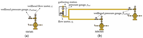
Figure 1.
The schematics of the (a) single-well-monitor system (SWMS) and (b) multi-well-monitor system (MWMS).
Generally, in the absence of the production data of a single well, several models can be established to calculate the production. For instance, the inflow performance relationship and hydraulic lifting curves [3,4,5,6,7], reservoir response model, or tailored reservoir model [8,9,10], and the temperature–pressure models [11,12] can be used to calculate the production rate of a single well. However, the above models could not consider the constraint of the production of a multi-well-monitor system. Therefore, these models are not a real sense of the splitting method and are inapplicable to split the production of the MWMS. At present, the studies of splitting the production of the MWMS are still far from adequate. Only a few methods are reported in the existing literature. Kappos et al. proposed a production splitting method (PSM) for the surface pipe network system on the basis of a choke equation [13]. However, their method requires the system being equipped with throttles, which hinders its application in real field cases. Hamad et al. and Abdelmoula et al. introduced an empirical PSM with the aid of a second-grade polynomial equation [14,15]. In order to obtain accurate results for splitting the production, one needs to update the coefficients of their empirical equation for each specific reservoir. However, in practice, the production data are frequently not available for one to generate such empirical equations. In addition, one can also split the production of the MWMS with commercial software (PIPESIM). PIPESIM can split the production by assuming that the properties of the fluid are uniform from different wells. However, in practice, the wells of the MWMS can be drilled in different regions or different layers and the properties of the fluids of different wells can be very different, rendering PIPESIM inapplicable. According to the aforementioned argument, one can find that splitting the production of the MWMS is important to predict the recovery and optimize the production. However, the existing methods bear different deficiencies in real applications. It is imperative for us to develop an inclusive method to split the production of the MWMS. In this work, the author proposed a new method to split the production of the MWMS. In comparison to the existing methods, this proposed method does not require the industries installing extra equipment and can consider the different properties of the fluid from different production wells.
2. Methodology
2.1. Physical Model and Assumptions
Figure 2 illustrates a simplified MWMS with two pipelines. In this figure, p represents pressure (psi), L represents the length of the pipeline (ft), the subscript “1” and “2” represent the first and the second pipeline, the subscript “g” and “l” represent the gas phase and liquid phase, respectively. p1, p2, and pout represent the wellhead pressure of well1, well2, and the outlet. qgt and qlt represent the total gas and liquid flow rate (scf/d, cubic ft/d). As we have introduced in Section 1, the values of L1, L2, p1, p2, pout, qgt, and qlt are known, and the values of qg1, ql1, qg2, and ql2 are the unknowns.
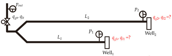
Figure 2.
Simplified model of an MWMS with two pipelines.
In order to develop the method for splitting the production of the MWMS, we made the following assumptions:
- The appearance of a curved section along the pipeline will not induce extra pressure drop;
- The temperature along the pipeline is linearly decreased from Twellhead at the wellhead to Tout at the outlet;
- The pipelines have the same properties, and these properties remain unchanged through the calculation.
2.2. Framework of the Proposed Method
In this section, we will take a two-well-monitor-system, as shown in Figure 2, as an example to illustrate the calculating process for splitting the production. This method is developed with a trial algorithm. The detailed introduction of the proposed method is as follows:
- Dividing the total gas flow rate into ng gas flow rates that have the same interval. The minimum gas flow rate is 0 and the maximum gas flow rate is qgt. In a similar way, dividing the total water flow rate into nw water flow rates. Arranging these ng gas flow rates and nw water flow rates into ng × nw flow rate pairs;
- Assuming that the gas flow rate of the first pipe is qg1 (scf/d) and the water flow rate of the first pipe is qw1 (cubic ft/d) (qg1 is one of the ng gas flow rates and qw1 is one of the nw water flow rates). According to the theory of mass balance, the gas flow rate and water flow rate of the second pipe can be calculated with:
- Calculating the pressure loss along the two pipes with the gas and water flow rate. The detailed process for calculating the pressure loss along a pipe will be introduced in the next section;
- Calculating the pressure loss along the two pipes with all the ng × nw pairs of flow rate, such that we can obtain ng × nw pressure loss of the two pipes;
- Graphing the pressure loss of the two pipes with these flow rate pairs in 3D graphs, as shown in Figure 3. Figure 3a,b shows the pressure loss graphs of the first pipe and the second pipe, respectively. In Figure 3a,b, the x-axis represents the gas flow rate of the first pipe qg1, the y-axis represents the water flow rate of the first pipe qw1, and the z-axis represents the pressure loss ∆p;
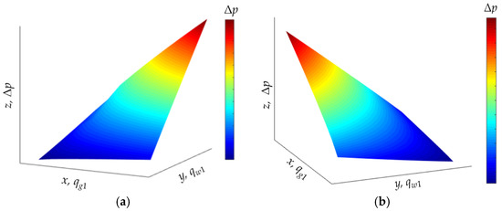 Figure 3. The pressure loss of the two pipes with different flow rate pairs: (a) the first pipe; (b) the second pipe.
 - Since the pressure losses of the two pipes are known, we can obtain all the possible values of qg1 and qw1 that can induce such pressure loss by intersecting the planes of z = ∆p1 and z = ∆p2 with the pressure-loss planes shown in Figure 3, as shown in Figure 4. The lines that are induced by the intersection represent all the possible values of qg1 and qw1;
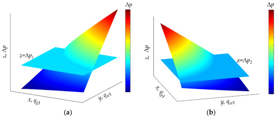 Figure 4. Intersection between the planes of z = ∆p1 and z = ∆p2 and the pressure-loss planes: (a) the first pipe; (b) the second pipe.
 - Figure 5a,b shows the x–y plane view of the possible-value lines of the two pipes, as shown in Figure 4. It should be noted that a reasonable value of qg1 and qw1 should ensure that the pressure loss of the first pipe equals to ∆p1 and the pressure loss of the second pipe equals to ∆p2. For example, (qgi, qwi) indicates a point on the intersection line in Figure 5a but not on the intersection line in Figure 5b. This indicates that flow rate pair (qgi, qwi) can lead to a pressure loss of ∆p1 for the first pipe, but it cannot lead to a pressure loss of ∆p2 for the second pipe. Therefore, this flow rate pair is not reasonable. The reasonable flow rate pairs can be found by intersecting the possible-value line in Figure 5a and the possible-value line in Figure 5b, as shown in Figure 5c;
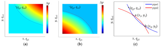 Figure 5. Obtaining the reasonable flow rate pairs by intersecting the two intersection lines: (a) the x−y plane view of the possible-value lines of the first pipe; (b) the x−y plane view of the possible-value lines of the second pipe; (c) the reasonable flow rate pairs.
 - The intersections in Figure 5c indicate the two reasonable flow rate pairs that can lead to a pressure loss of ∆p1 for the first pipe and a pressure loss of ∆p2 for the second pipe. One can figure out the real flow rate pair from these two reasonable flow rate pairs on the basis of the development strategy and reservoir properties. For example, if the first pipe is connected to a reservoir/layer that has a higher initial water saturation than that of the second pipe, the water flow rate of the first pipe can be higher than that of the second pipe. Hence, one can think that the flow rate pair b (x2, y2) in Figure 5c is the real flow rate pair of the first pipe. Additionally, the flow rate of the second pipe is qgt-x2 and qwt-y2.
2.3. Method of Calculating the Pressure Loss along a Pipeline
The multiphase flow in pipelines can illustrate different flow patterns with different flow velocity, which makes it complicated to calculate the pressure loss along the pipeline. One of the most commonly used methods to calculate the pressure change along the pipes accounting for the different flow patterns is the Beggs and Brill (BB) correlation. In the BB correlation, the fluid flow is divided into three patterns, including segregated flow, intermittent flow, and distributed flow [16]:
Segregated flow: the segregated flow is a flow regime in a pipeline where the different phases of fluid are segregated, as shown in Figure 6a. Specifically, the segregated flow includes three sub-patterns, namely stratified flow, wavy flow, and annular flow;
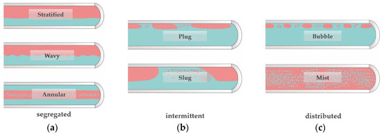
Figure 6.
Schematics of different flow patterns: (a) segregated flow; (b) intermittent flow; (c) distributed flow.
Intermittent flow: if the gas–liquid ratio is sufficiently high, the gas phase will be observed in the form of plugs or slugs, as shown in Figure 6b, and the intermittent flow contains the sub-patterns of plug flow and slug flow;
Distributed flow: the distributed flow contains bubble flow and mist flow, as shown in Figure 6c. The bubble flow happens to the scenarios of a low gas–liquid ratio, and the mist flow happens to the scenarios of a high gas–liquid ratio.
In addition, since the properties of the fluid and the flow pattern are highly dependent on the pressure and temperature, both the properties of the fluid and the flow pattern will be changed along the pipe as the pressure and temperature are changed along the pipe. In practice, all the flow patterns can be observed in the real field cases under different conditions of pressure and temperature. In order to characterize the varied flow pattern and the varied fluid properties, we need to discretize the pipe into small segments. Figure 7 shows the schematic of a discretized pipe. As shown in this figure, the fluid flows into the pipe through the inlet surface and flows out of the pipe through the outlet surface.
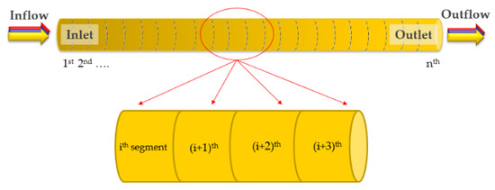
Figure 7.
Schematic of a discretized pipe.
Figure 8 shows the detailed process of calculating the pressure loss in a discretized pipe. The flow properties and pressure loss in the pipeline are calculated iteratively:
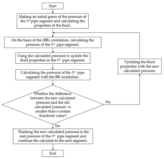
Figure 8.
Flow chart of the process for calculating the pressure of a discretized pipe.
- Making an initial guess of the pressure of the 1st pipe segment. For example, one can use the pressure at the inlet surface as the initial guessed pressure of the 1st segment. Calculating the properties of the fluid with the guessed pressure by use of the equations in Appendix A;
- On the basis of the BB correlation, identifying the flow pattern in the 1st pipe segment and calculating the new pressure within the 1st pipe segment. The introduction of the BB correlation can be found in Appendix B;
- Using the calculated pressure to update the fluid properties and flow pattern in the 1st pipe segment and calculating the pressure of the 1st pipe segment with the BB correlation;
- If the difference between the new calculated pressure and the old calculated pressure is smaller than a certain threshold value, one can think that the new calculated pressure is the real pressure of the 1st pipe segment; otherwise, updating the fluid properties with the new calculated pressure and repeating the calculating. In this work, if the absolute value of the relative difference between the new pressure and the old pressure is smaller than 0.0001, we think the new calculated pressure is the real pressure;
- Calculating the pressure of the next pipe segment with a similar method that is introduced in Steps 1 through 4. For the nth segment, one can use the pressure of the (n − 1)th segment as the initial guess.
3. Validation of the Proposed Method
In this section, we applied this proposed method to an MWMS in the Hechuan Gas Field in China. The gas production Wells X1 and X2 are in the same well group, and the production of these two wells are transmitted with two separate pipes. The properties of the pipes and the schematic of the MWMS are shown in Table 1 and Figure 9.

Table 1.
The properties of the pipes and the measured data.
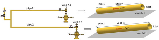
Figure 9.
Schematic of an MWMS and the pipes.
Figure 10 shows the gas production rate of Well X1, X2, and well group of 30 days, as shown in Figure 10a, and the water production rate of X1, X2, and well group of 30 days, as shown in Figure 10b. Figure 11 presents the wellhead pressure of these two wells, as well as the outlet pressure of 30 days. Therefore, we can split the production of these two wells with the proposed method by use of the total gas and water production rate together with the wellhead pressure and outlet pressure. Subsequently, this proposed method can be validated by comparing the calculated results to the real measured data. In order to conduct a more thorough comparison, we also use the commercial software PIPESIM to split the production.
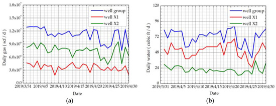
Figure 10.
The (a) daily gas production data and (b) daily water production data of the well group for 30 days.
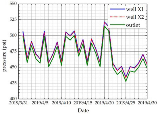
Figure 11.
The outlet pressure and the wellhead pressure of these two wells of the 30 days.
As introduced in Section 2, we calculated all the possible production rates with the trial algorithm and obtained the two reasonable production rate pairs by intersecting the possible-value lines of Well X1 and that of Well X2. Figure 12 shows the possible-value lines of Well X1, X2, and their intersections of the first five days. The reasonable production rate pairs of the other 25 days can be obtained with the same method.
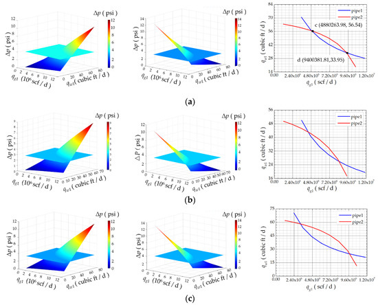
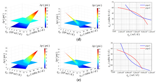
Figure 12.
Obtaining the reasonable flow rate pairs of the first 5 days: (a) 1st day; (b) 2nd day; (c) 3rd day; (d) 4th day; (e) 5th day.
Table 2 summarizes the values of the reservoir parameters of Well X1 and X2. As one can see in Table 2, the porosity, initial gas saturation, and reservoir thickness of the reservoir of Well X2 are all higher than those of Well X1. Therefore, one can infer that the gas production rate of Well X2 can be higher than that of Well X1. With such a constrained condition, the right production rate pair can be identified from the two reasonable production rate pairs. For example, as one can see in Figure 12a, there are two reasonable production rate pairs of Well X1, c (4,880,263.98 scf/d, 56.54 cubic ft/d), and d (9,400,381.81 scf/d, 33.95 cubic ft/d) in the first day. Therefore, the reasonable production rate pairs of Well X2 are (8,016,020.03 scf/d, 26.02 cubic ft/d) and (3,495,902.20 scf/d, 48.61 cubic ft/d). Finally, we chose the first production rate pair c as the real production rate pair of Well X1.
Table 2.
Values of reservoir parameters of Well X1 and Well X2.
Figure 13 demonstrates the calculated results from this proposed method, the calculated results from PIPESIM, and the real field data. Figure 13a,b shows the gas production and water production of the two wells, respectively. As one can see in Figure 13, that although both the results from the proposed method and those from PIPESIM undergo good agreement with the real field data for splitting the gas production, as shown in Figure 13a, this proposed method exhibits a better performance than PIPESIM for splitting the water production, as shown in Figure 13b.
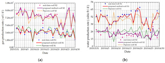
Figure 13.
Comparison between the results of the proposed method, the results from PIPESIM, and the real field data: (a) comparison of the gas production data; and (b) comparison of the water production data.
Figure 14 compares the relative errors re of this proposed method to those of PIPESIM. The relative error is defined as
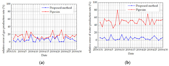
Figure 14.
The relative errors of this proposed method and those of PIPESIM: (a) relative error of gas production rate; (b) relative error of water production rate.
The relative errors of the gas and water production rate of the 30 days are shown in Figure 14a,b. As one can see in Figure 14, the relative error induced by the proposed method is less than that induced by PIPESIM. The average relative errors of the gas production rate calculated by the proposed method and PIPESIM are 6.59% and 15.79%, respectively. The average relative errors of the water production rate calculated by the proposed method and PIPESIM are 5.39% and 50.56%, respectively. The results shown in Figure 13 and Figure 14 indicate that this proposed method is reliable for splitting the production of the MWMS.
4. Sensitivity Analysis
In this section, we conducted a study of the effects of different influencing factors on the calculation outputs. These influencing factors include the inner diameter of the pipes, the absolute roughness of the inner wall of the pipes, and the pressure loss along the two pipes. Since only three influencing factors are examined in this work, the computation load is not heavy, and the computation can be completed in a few seconds. In practice, if more influencing factors are required to be investigated and the computation load is heavy, one can use the software framework that is developed by Vu-Bac et al. [17] to conduct the sensitivity analysis. The benchmark values of the properties of the pipes and the pressure are the same as those used in Section 3.
4.1. The Inner Diameter of Pipes
Figure 15 shows the effect of the inner diameter of the second pipe on the results of production splitting. In Figure 15, the inner diameter of the second pipe is varied from 0.195 ft to 0.202 ft. As one can see in Figure 15, as the inner diameter of the second pipe is increased, the gas production of the second pipe is decreased, while the water production of the second pipe is increased. This can be explained as follows. The gas production of the two wells is significantly higher than the water production rate and the pressure loss along the pipes is mainly induced by the gas flow. Compared with the pressure loss that is induced by the gas flow, the pressure loss that is induced by the water flow is very small. Increasing the inner diameter of a pipe while leaving the flow rate unchanged will reduce the difference between the pressure of the inlet surface and that of the outlet surface, whereas increasing the inner diameter of a pipe while leaving the pressure difference unchanged will reduce the gas flow rate. In Figure 15, the pressure difference remains unchanged during the computation; hence, the gas flow rate is decreased while the water flow rate is increased as the inner diameter of the second pipe is increased.
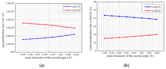
Figure 15.
Calculation results under different inner diameter of pipes: (a) gas production rate; (b) water production rate.
4.2. The Absolute Roughness of Pipes
Figure 16 shows the split gas and water production rates under different absolute roughness of pipes. It can be observed in Figure 16, as the absolute roughness of the pipe is varied from 10−4 ft to 10 ft, the gas production and the water production of the two wells show negligible change. This indicates that the absolute roughness of the pipe can slightly influence the results of the production splitting.
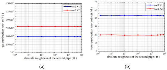
Figure 16.
Calculation results under different absolute roughness of pipes: (a) gas production rate; (b) water production rate.
4.3. The Pressure Loss of Pipes
Figure 17 shows the gas and water production rates of the two wells with a different pressure loss of the second pipe. As we have stated in Section 4.1, the pressure loss is mainly caused by the gas flow, and a larger pressure loss indicates a higher gas flow rate of the pipe. Therefore, in Figure 17 we can find that the gas flow rate is increased, while the water flow rate is decreased as the pressure loss of the second pipe is increased.
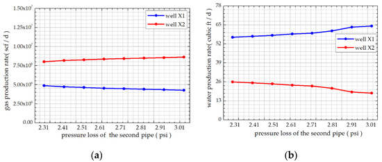
Figure 17.
Calculation results under different pressure loss combinations: (a) gas production rate; (b) water production rate.
5. Conclusion
In this work, the authors proposed a new method to split the production of the MWMS. This method is constructed on the basis of a trial method and the BB correlation. In order to accurately characterize the flow patterns and the fluid properties along the pipeline, we discretized the pipeline into small segments and identified the flow pattern within each small segment. In comparison to the existing methods for splitting the production, this proposed method does not necessitate installing measuring equipment and can consider the different properties of the fluid from different wells. However, this method can induce multiple reasonable solutions, and one needs to recognize the real solution from the multiple solutions based on the field data. This proposed method was validated against field monitored data. The calculated results from this proposed method show excellent agreement with those of the field data, indicating that this proposed method is reliable to split the production of the MWMS. Besides, we also compared the results from this proposed method to those from commercial software PIPESIM, and the results show that this proposed method can yield more accurate results for splitting the production.
Author Contributions
Conceptualization, J.Z. and C.H.; methodology, B.T.; software, X.L. and C.H.; validation, W.L.; formal analysis, B.T.; investigation, J.Y.; resources, W.L.; data curation, J.Z.; writing—original draft preparation, J.Z.; writing—review and editing, B.T.; visualization, J.Z.; supervision, J.Y.; funding acquisition, W.L. All authors have read and agreed to the published version of the manuscript.
Funding
This research was funded by National Natural Science Foundation of China, grant number 51674227.
Acknowledgments
The authors would like to thank National Natural Science Foundation of China for the support and promotion.
Conflicts of Interest
The authors declare no conflict of interest. The funders had no role in the design of the study; in the collection, analyses, or interpretation of data; in the writing of the manuscript, or in the decision to publish the results.
Appendix A
The pseudocritical pressure and temperature can be calculated with the following equations [18]:
where ppc is the pseudocritical pressure of gas (psi), Tpc is the pseudocritical temperature of gas (°R), and γg is the specific gravity for gas.
Using the obtained pseudocritical pressure and temperature, the reduced pressure pr, temperature Tr, and dimensionless density of gas ρr can be calculated [18]:
where T is temperature (°R), p is pressure (psi).
The gas formation volume factor Bg can be calculated using the real gas equation:
where psc is pressure at standard conditions (psi) and Tsc is temperature at standard conditions (°R).
Using the Dranchuk and Abou-Kassem equation [19], which is based on the generalized Starling equation of state to calculate the gas-deviation factor z:
where the values of constants A1 through A11 are shown in Table A1.
Table A1.
Values of the constants.
Table A1.
Values of the constants.
| Constants | Value |
|---|---|
| A1 | 0.3265 |
| A2 | −1.0700 |
| A3 | −0.5339 |
| A4 | 0.01569 |
| A5 | −0.05165 |
| A6 | 0.5475 |
| A7 | −0.7361 |
| A8 | 0.1844 |
| A9 | 0.1056 |
| A10 | 0.6134 |
| A11 | 0.7210 |
Using the following equations [20] to calculate the viscosity of gas μg (cp):
where
where ρ is gas density (g/cm3), K1 is parameter (cp), and Mg is average molecular weight of gas.
Appendix B
The Bernoulli equation characterizes the fluid flows in pipelines by considering the effects of kinetic pressure loss, hydrostatic pressure loss, and frictional pressure loss. Since the kinetic loss is normally much smaller than the hydrostatic loss and friction loss, the kinetic loss can be neglected, and the Bernoulli equation can be simplified as
where ∆pT is total pressure loss (psi), ∆pH is hydrostatic pressure loss (psi), and ∆pf is friction pressure loss (psi). The parameters used for characterizing the multi-phase flow are given as follows:
where ql is the flow rate of liquid-phase (ft3/d), qw is the flow rate of water (ft3/d), qg is the flow rate of gas (ft3/d), Bw is the water volume factor, Bg is the gas volume factor, Vsl is the superficial velocity of liquid (ft/d), Vsg is the superficial velocity of gas (ft/d), Vm is the superficial velocity of mixture (ft/d), and D is the diameter of pipe (ft). It is worth noting that the formation volume factor Bw and Bg indicate the ratio of the fluid volume in the pipe to the fluid volume of the standard condition.
Figure A1 shows the schematic of multiphase flow in a pipe. Due to the change of the pressure, the gas phase will be compressed or expanded along the pipeline, leading to a variation of the volume fraction of the gas phase at different cross-sections of the pipelines. Liquid holdup El refers to the proportion of the liquid phase’s cross-sectional area Al (ft2) in the total cross-sectional area AP (ft2) during the water–gas two-phase flow. El can be defined as follows:
If the slippage effect is neglected, no-slip holdup Cl can be obtained:
In this work, we used the Beggs and Brill (BB) correlation to calculate the pressure loss along the pipelines. The BB correlation is applicable to the wells with arbitrary inclinations and can account for the change of flow pattern. In the BB correlation, the flow patterns are summarized into three groups of flow, including segregated flow (including stratified, wavy, and annular flow), intermittent flow (including plug and slug flow), and distributed flow (including bubble and mist flow). Before calculating the pressure loss with the BB correlation, the flow pattern is required to be recognized if the values of no-slip holdup Cl and Froude number Frm are known prior. The Froude number Frm is defined as [16]
The boundaries between these groups of flow patterns appear as curves in a log-log plot in the original publication by Beggs and Brill. Beggs and Brill (1973) fitted the boundary lines in a log-log plot in order to facilitate the process of determining the flow patterns, which can be summarized as follows.
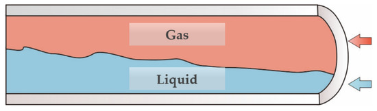
Figure A1.
Schematic of multiphase flow in a pipe.
If Frm < L1*, the flow pattern falls within the segregated flow, if Frm > L1* and Frm > L2*, the flow pattern falls within the distributed flow, if L1* < Frm < L2*, the flow pattern falls within the intermittent flow. L1* and L2* are given by:
where
Once the flow pattern is determined, the liquid holdup El can be calculated. The liquid holdup El in the BB correlation contains two parts, including a liquid holdup of horizontal flow El(0) and a correction coefficient that accounts for the inclination angle. The value of the horizontal liquid holdup El(0) should not be less than the value of the no-slip holdup Cl. In the case of El(0) < Cl, one can set El(0) = Cl.
If the flow pattern falls within the segregated flow. In such cases, one can have [16]:
In addition, if the flow pattern is intermittent flow:
If the flow pattern is dispersed flow:
Once the flow pattern is determined and the horizontal liquid holdup El(0) is obtained, the real liquid holdup El that considers the inclination angle can be calculated with a correction coefficient B(θ):
where
where β is a function that is dependent on the flow pattern as well as the flow direction of the fluid.
If the flow direction is uphill, for segregated flow, we can have:
for intermittent flow:
for distributed flow:
If the flow direction is downhill flow (all flow patterns), we can have:
for all flow patterns, where NLv is the liquid velocity number, which is defined as
where σ is liquid surface tension and ρl is liquid density.
With the aid of Equations (A24) through (A33), the real liquid holdup El can be obtained. The density ρm (lb/ft3) and the viscosity μm (cp) of the mixture in the pipeline can be calculated with:
The hydrostatic pressure loss ∆pH (psi) that is caused by the gravity can be calculated with:
where gc is the gravitational constant, and θ is the inclination angle with respect to the horizontal direction. For example, for the vertical direction θ = 90°, and for horizontal direction θ = 0°.
The pressure loss ∆pf (psi) that is caused by the friction can be calculated with:
In Equation (A37), ftp and ρNS (lb/ft3) are the two-phase friction coefficient and no-slip density, respectively. ftp and ρNS are defined as follows:
where
If the fluid composition in the pipe is known, using Equations (A19) through (A23) can determine the flow pattern of fluid. Subsequently, one can calculate the pressure loss that is induced by gravity and friction with Equations (A24) through (A43).
References
- Wei, G.; Xie, Z.; Li, J.; Yang, W.; Zhang, S.; Zhang, Q.; Liu, X.; Wang, D.; Zhang, F.; Cheng, H. New research progress of natural gas geological theories in China during the 12th Five-Year Plan period. Nat. Gas Ind. B 2018, 5, 105–117. [Google Scholar] [CrossRef]
- Wang, S. Shale gas exploitation: Status, problems and prospect. Nat. Gas Ind. B 2018, 5, 60–74. [Google Scholar] [CrossRef]
- Liao, T.T.; Lazaro, G.E.; Vergari, A.M.; Schmohr, D.R.; Waligura, N.J.; Stein, M.H. Development and Applications of Sustaining Integrated Asset Modeling Tool. SPE Prod. Oper. 2007, 22, 13–19. [Google Scholar] [CrossRef]
- Leskens, M.; Smeulers, J.P.M.; Gryzlov, A. Downhole Multiphase Metering in Wells by Means of Soft-sensing. In Proceedings of the Intelligent Energy Conference, Amsterdam, The Netherlands, 25–27 February 2008. [Google Scholar]
- Muradov, K.M.; Davies, D.R. Zonal Rate Allocation in Intelligent Wells. In Proceedings of the EUROPEC/EAGE Conference, Amsterdam, The Netherlands, 8–11 June 2009. [Google Scholar]
- Kabir, A.H.; Sanchez Soto, G.A. Accurate Inflow Profile Prediction of Horizontal Wells through Coupling of a Reservoir and a Wellbore Simulator. In Proceedings of the SPE Reservoir Simulation Symposium, The Woodlands, TX, USA, 2–4 February 2009. [Google Scholar]
- Yoshioka, K.; Zhu, D.; Hill, A.D. A New Inversion Method to Interpret Flow Profiles From Distributed Temperature and Pressure Measurements in Horizontal Wells. SPE Prod. Oper. 2007, 24, 510–521. [Google Scholar] [CrossRef]
- Von Schroeter, T.; Hollaender, F.; Gringarten, A.C. Deconvolution of Well-Test Data as a Nonlinear Total Least-Squares Problem. SPE J. 2004, 9, 375–390. [Google Scholar] [CrossRef]
- Levitan, M.M. Practical Application of Pressure-Rate Deconvolution to Analysis of Real Well Tests. SPE Reserv. Eval. Eng. 2005, 8, 113–121. [Google Scholar] [CrossRef]
- Levitan, M.M.; Crawford, G.E.; Hardwick, A. Practical Considerations for Pressure-Rate Deconvolution of Well Test Data. SPE J. 2006, 11, 35–47. [Google Scholar] [CrossRef]
- Ramey, H.J. Wellbore Heat Transmission. J. Pet. Technol. 1962, 14, 427–435. [Google Scholar] [CrossRef]
- Rasoul, R.R.A.; Refaat, E. A Case Study: Production Management Solution “A New Method of Back Allocation Using Downhole Pressure and Temperature Measurements and Advance Well Monitoring”. In Proceedings of the SPE/DGS Saudi Arabia Section Technical Symposium, Al-Khobar, Saudi Arabia, 15–18 May 2011. [Google Scholar]
- Kappos, L.; Economids, M.J.; Buscaglia, R. A Holistic Approach to Back Allocation of Well Production. In Proceedings of the SPE Reservoir Characterisation and Simulation Conference, Abu Dhabi, UAE, 9–11 October 2011. [Google Scholar]
- Hamad, M.; Sudharman, S.; Al-Mutairi, A. Back Allocation System with Network Visualization. In Proceedings of the Abu Dhabi International Conference, Abu Dhabi, UAE, 10–13 October 2004. [Google Scholar]
- Abdelmoula, D.; Dunlop, J.E.M. Qatargas Well Production Back Allocation Project—Methodology & System Requirements. In Proceedings of the International Petroleum Technology Conference, Doha, Qatar, 6–9 December 2015. [Google Scholar]
- Beggs, D.H.; Brill, J.P. A Study of Two-Phase Flow in Inclined Pipes. J. Pet. Technol. 1973, 25, 607–617. [Google Scholar] [CrossRef]
- Vu-Bac, N.; Nguyen-Thoi, T.; Rabczuk, T. A software framework for probabilistic sensitivity analysis for computationally expensive models. Adv. Eng. Softw. 2016, 100, 19–31. [Google Scholar] [CrossRef]
- Sutton, R.P. Compressibility Factors for High-Molecular-Weight Reservoir Gases. In Proceedings of the SPE Annual Technical Conference, Las Vegas, NV, USA, 22–26 September 1985. [Google Scholar]
- Hall, K.; Yarborough, L. A new equation of state for Z-factor calculations. Oil Gas J. 1973, 71, 82–92. [Google Scholar]
- Lee, A.L.; Gonzalez, M.H.; Eakin, B.E. The Viscosity of Natural Gases. J. Pet. Technol. 1966, 18, 997–1000. [Google Scholar] [CrossRef]
Publisher’s Note: MDPI stays neutral with regard to jurisdictional claims in published maps and institutional affiliations. |
© 2020 by the authors. Licensee MDPI, Basel, Switzerland. This article is an open access article distributed under the terms and conditions of the Creative Commons Attribution (CC BY) license (http://creativecommons.org/licenses/by/4.0/).