Simplified Assessment on the Wind Farm Noise Impact of the E²O Experimental Offshore Station in the Asturian Coast

Abstract

This paper presents a preliminary evaluation of the acoustic impact of an offshore experimental wind farm (E²O), conceived and planned to be installed in Asturias on Spain’s northwest coast. A simplified assessment of the wind turbines’ noise impact at an offshore platform was performed numerically, adapting commercial software for room acoustics to this particular application. As a result, the sound levels at specific receiver sites on the coastline were estimated to select the most convenient level between the two possible locations. Parameters from acoustic emission data of the selected wind turbines were introduced as inputs to the simulation, and the noise propagation in the analyzed domains (for different values of their basic parameters) was simulated. Complementarily, the numerical results were compared to calculations following the ISO 9613-2 standard on sound propagation outdoors for validation purposes, showing good overall agreement. The results revealed that both projected areas under consideration follow the current normative concerning the prescribed acoustic limits, according to the predicted low sound pressure values at the specific considered receiver sites.

1. Introduction

In recent years, the percentage of offshore wind farms has increased worldwide compared to the total installed wind energy capacity. They are expected to be some of the most important structures for the future energy supply due to a number of advantages compared to onshore structures: the roughness of the water is lower, the wind velocity is higher, turbulence effects are lower, there are great extensions of marine surfaces available and the visual and acoustic impact on the population is reduced. However, offshore wind farms have some disadvantages, among which the most negative comprise the lack of an electrical control module to connect them to the grid and the higher maintenance and foundation costs involved.

Wind farms’ operating companies have increased their interest in noise impact due to resistance from people settling in the proximity of new projects. Van den Berg [1] presented a vision of residential health effects in relation to wind turbine noise. Relevant correlations were found regarding noise discomfort, such as sleep disorder and stress. Janssen et al. [2] derived the relationship between exposure and wind turbine noise and the expected percentage of annoyed residents, comparing it to previously established industrial and transportation noise relationships. It was reported that, in comparison to other sources of environmental noise, annoyance due to wind turbine noise was found even at relatively low noise exposure levels. Bakker et al. [3] also carried out a study to determine the relationship between exposure to sound from wind turbines and inhabitants’ discomfort, such as annoyance, sleep disturbance and psychological distress. They concluded that people living close to wind farms are at risk of being annoyed by the noise, which must be considered a relevant adverse effect. Other authors have studied complementary aspects related to the wind turbine noise impact, such as Maffei et al. [4]. In particular, they analyzed the effects of vision-related aspects on noise perception for wind turbines in quiet areas using the immersive virtual reality technique. Similarly, Bishop et al. [5] investigated the influence of distance, contrast, movement and social variables in offshore wind turbine locations. In conclusion, the noise produced by wind turbines is considered one of the main limitations to the widespread development of wind energy. Therefore, acoustic analysis of wind farms is an important topic that must be assessed in order to advance in the development of wind energy technologies.

As an example, Zhao et al. [6] recently presented results on a noise impact assessment for a proposal of a 30 MW wind farm in Lake Erie in Ontario, Canada. This report reviews noise issues of a wind farm, sound propagation and the major factors that might affect the sound propagation and noise modeling results. The software-based calculation for noise impact is based on the ISO 9613-2 standard on sound propagation outdoors [7]. Kaldellis et al. [8] presented and evaluated a set of real experimental noise measurements derived from a small wind farm. The obtained measurements were compared to simulation results given by applying two software tools, one of them based on the ISO 9613-2 standard. Bolin et al. [9] studied the propagation of sound from a wind turbine using analytical and computational calculations. Similar studies by Delaire et al. [10] and Guarnaccia et al. [11] used two different techniques. Larsson et al. [12] studied how meteorological effects perturb sound propagation, while other authors, such as Andersson et al. [13], investigated the effects of turbulence on sound propagation from a wind turbine site at sea.

Nowadays, most limits on wind turbine noise prevent exceeding the limit of 35 or 40 dBA as long as they do not exceed the background noise level at neighboring areas by more than a specified amount, often 5 dBA [14].

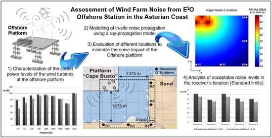
Considering such ideas, a preliminary evaluation of the acoustic impact of an offshore experimental wind farm, conceived and currently under consideration to be installed in Asturias on Spain’s northwest coast, was conducted. The facility is an initiative of the University of Oviedo (through its Campus of International Excellence) in collaboration with the Cluster of Energy, Environment and Climate Change, an entity responsible for the E²O project for the creation of an Offshore Experimental Station. The Offshore platform is intended to be a large-scale “test lab” for conducting marine research focusing on offshore energy generation devices, such as seabed and floating devices like buoys, pelamis, tidal energy converters and wind turbines. Other types of studies and experiments will also be carried out in the site, such as weather, aquaculture and material testing or oceanography, among others. This station will be specialized in the generation, storage and transportation of marine energy and allow testing equipment in real operating conditions on the Asturian coast.

As part of the preliminary studies, two possible locations of the E²O Offshore Experimental Station were studied in this investigation for its final settlement. The previous selection of the two candidate locations of the lab was made according to the following criteria: capability for electrical connection, affordable depth, geological constraints for foundations, meteorological characteristics and distance to the coastline. Additional aspects related to ocean currents, such as height and wave period in the two studied places, were also considered.

In the present investigation, a simplified noise impact assessment for an offshore wind farm platform was numerically carried out using a noise propagation model. Sound power levels for selected wind turbines were introduced according to the manufacturer noise data. The sound levels at different receivers of interest on the coastline were finally estimated according to the results of the propagation model. A validation with analytical calculations provided by the ISO S9613-2 standard was also carried out, and sensitivity studies regarding propagation coefficients were considered for a major insight.

2. Methodology

Commercial software to handle acoustic performance studies (Odeon Room Acoustics) was adapted to numerically perform a simplified assessment of the wind turbines’ noise level to be installed on the offshore platform. This general-purpose commercial program was reoriented to study a specific outdoor problem using a rational selection of physical and geometrical parameters for the following calculations: boundary conditions, mesh sizes, propagation model, reflection and refraction parameters at the boundaries and frequencies of interest. To do so, sound power levels for the selected wind turbines were introduced into the sources’ noise emission model, and their propagation in the modeled domains was simulated using a noise propagation model. As a result, the sound levels at different receivers of interest on the coastline were estimated to select the most convenient of the two locations. The obtained results were compared, for validation purposes, to analytical calculations in accordance with the ISO 9613-2 standard on sound propagation outdoors, showing an overall good agreement. Sensitivity studies were performed regarding scattering coefficients to observe the influence of the change in baseline parameters on the final results.

Two possible locations for the E²O Offshore Experimental Station, which is to be installed on the Asturian coastline (Cantabrian Sea) on Spain’s north coast, were considered in the present investigation. Preliminary studies for possible locations were developed by the Cluster of Energy, Environment and Climate Change, including the analysis of different selection criteria (energetic, operational, geographic, geological and meteorological) with a direct impact on the convenience of the site. The two final candidate locations for the offshore platform are Cape Busto, 43°33′51″ N–6°29′11″ W, and Llumeres, 43°39′3″ N–5°49′33″ W (GPS coordinates refer to the closest point to the coastline).

Figure 1 shows the location map and simulated geometry for the first possible location, named the Cape Busto platform, while Figure 2 shows the situation map and simulated geometry for the second location, named the Llumeres platform. In these figures, all distances are expressed in meters. The Cape Busto platform is a rectangular area, located at a minimum distance of 1375 from the coast, while the Llumeres platform is an L-shaped area, located at a minimum distance of only 800 m from the coast. Both platforms are located within shallow water (30–50 m) where the seabed and floating devices will be tested. The nominal characteristics of the platforms can be summarized according to the following data: a total area of 3.5 km² (1 nautical mile × 1 nautical mile) at approximately 2 km from the coast and with a maximum water depth of 50 m.

To simulate the sound propagation, a simplified model of the coastline was considered (transparent blocks representing sand and concrete zones in Figure 1 and Figure 2). This feature was adopted because it is expected that a higher mesh resolution would not imply significant changes in the noise maps, and the time required to complete the simulations would be significantly higher (extensive details of the geometry would imply extremely fine meshes with excessive CPU times). Numerical results have effectively confirmed uncertainties in the range of ±2 dBA (A-weighted decibels), which are perfectly assumable for this preliminary study, in positions all along the coastline where variations in noise propagation are perceived. More details are given below in the Results and Discussion section. Furthermore, the possible elevations existing between the coastline and receivers, located 50 m away, were considered to be negligible because, in both platforms, the land is almost flat and there are no natural barriers associated with the presence of woody vegetation. The receivers were precisely located 50 m from the shoreline because this is the minimum possible distance allowed by Spanish regulations to construct buildings. Between the receivers and the offshore wind turbines, there are no obstacles that may attenuate or modify noise propagation, although properly targeted air circulation on the coastal and wind turbulence zones can modify the propagation and intensity of noise. The receivers were located 4 m above ground level, the reference height indicated by the 2002/49/CE European Directive [15], to be used during the measurement and mapping of noise impact assessments.

Under the financial support of the E²O project, it was planned to install up to three wind turbines at the Cape Busto platform and up to five at the Llumeres platform, with a maximum installed capacity of 10 MW. All wind turbines are of the G90 type (from GAMESA, one of the world-leading wind turbine manufacturers), and the main characteristics are summarized in

Table 1. G90 wind turbine characteristics.

G90 Wind Turbine
Rotor diameter	90 m
Swept area	6362 m2
Speed	9–19 rpm
Tower height	100 m
Rated power	2000 kW
Generator voltage	690 V
Rotational speed at 50/60 Hz	1680/2016 rpm

. The G90 is a 2 MW, three-bladed, windward pitch-regulated and active yaw wind turbine. It was certified as Class IIIA and DIBt WZ II, according to the IEC 61400-1 [16]. The turbine blades are DU-FFA-W3 airfoils, 44 m in length, bolted to a hub at the low-speed end of a 1:120 ratio gearbox. As shown in this table, the G90 turbine has a rotor diameter of 90 m, giving a swept area of 6362 m². The hub height of the G90 wind turbines is placed 100 m over the sea level.

To implement these G90 wind turbines in the software for noise propagation, their total and A-weighted sound power levels were calculated from the data supplied by the manufacturer. These levels are shown in Figure 3 for a typical rotation speed of 15.3 of the wind turbines (corresponding to an 8 m·s⁻¹ wind velocity 10 m from the ground). These noise emissions were certified using IEC 61400-1 and are based on a normalization procedure of the amplitudes in order to compare the frequency distribution of wind turbines with different total sound pressure levels (SPLs) [17]. Notice that the levels of sound power levels for these wind turbines can be found in the frequency range between 500 and 1000 Hz. The total sound power reaches up to 100 dBA.

A commercial package for general purposes, Odeon Room Acoustics [18], whose software is based on the acoustic ray method, was tested in this study for the simulation of the wind turbine’s noise propagation. The program editor was used to generate the required geometries and the various surfaces shown previously in Figure 1 and Figure 2. Receivers were placed at the corresponding locations (as shown in Figure 4 and Figure 5) at the height of 4 m above ground level, as established by the Spanish regulation and the European directives.

Using the software, point sources representing the wind turbines were placed in the corresponding positions. In this step, sound power data calculated for each octave band were also loaded. In the Odeon program, a hybrid method is employed to calculate the sound level contributions from the point sources. The code resolves “early reflections” using the ray-tracing technique combined with an image source model, while “late reflections” are modeled introducing secondary terms at solid boundaries to track local energy radiation in the acoustic ray method. The following resolution algorithm starts searching for reflection paths that affect the location of any receiver independently (designated as “receiver independent part calculations”). Rays coming from point sources are equally distributed in all directions on a sphere. The geometrical data generated by the rays being reflected in the domain are then stored in terms of the total number of interactions with solid walls and incidence points. This is because the typical criterion for ray termination is geometrically based on either the path length traveled or the total reflections. Since “early reflections” are characterized by a different pattern (they are reflected specularly), their response is modeled depending on their reflection order: if this value is higher than the transition order, they are resolved using the Odeon module for late rays; otherwise, they are treated differently, introducing the detection algorithm for image sources. Once all the data concerning the different ray trajectories in the whole domain are available, the second part of the algorithm (termed “receiver dependent part calculations”) collects all the information of ray reflections at the specific points where the receiver is placed. At this stage, the final results for sound pressure levels at the desired locations are calculated using both direct and reflected contributions tracked in the previous step. In the case that several receivers are involved, the result for each receiver is obtained by repeating this dependent part as many times as necessary. Similarly, if several sources are present in the problem, the final solution is computed through the superposition of the individual contributions of each source, applying the corresponding delays as a function of the distance of the source to the receiver. More specifically, in the simulations carried out, the number of rays was set to 1000, with a maximum reflection order of 2000 and an impulse sound level contribution length of 2000 ms. In this preliminary phase of the noise impact calculations, in order to preserve a neutral scenario, the effect of wind direction and weather conditions has not been taken into account on the noise propagation towards the coastline.

For the embedded ground portion of water, the natural material water of the software library was used. To represent the coast, the same library of natural materials was selected using the material named sand. One completely absorbent material was used for the geometry boundaries in order to avoid wave reflections that may distort the results. This material is one of the special library materials. All these materials have predefined a scattering coefficient that represents a percentage of nonspecular reflection, which, in this case, was established at 0.05. Finally, the effects of all sources for punctual results and the spacing mesh were included in a specific process that was also programmed.

Since the offshore wind farms included in this project have not yet been installed, it has not been possible to calibrate the acoustic propagation model with experimental measurements for in situ validation. However, the acoustic ray method employed here is well known to provide accurate results when spherical propagation from a point source to receiver points is expected (like in the present case). Several reports analyzing similar situations for far-field propagation of wind turbine noise can be cited here as a reference [19,20,21,22]. In particular, these studies validate similar codes (Nord2000, CONCAWE, etc.) for noise propagation in offshore wind farms, concluding that, in the case of flat topologies, ray-tracing propagation methods provide very good agreement with in-place measurements [21]. Moreover, comparison with the analytical application of ISO 9613-2 is also a valid possibility in the literature as it provides reasonable predictions, although some evidence demonstrates that it usually underpredicts sound levels propagated for long distances over water [19]. This option was used for validation in Section 3 and the Appendix A, confirming that the ISO results slightly underpredict the noise propagation computed with the acoustic ray method.

The location of the sources is a very important issue because a wind turbine that is placed in the wake of another may produce less power due to the aerodynamic shadow of the upstream turbine. On the other hand, having relatively small distances between turbines allows installing a larger number of turbines but reduces the power rated by each in the wind farm. Aerodynamic losses can be reduced by optimizing the geometry of the wind farm, since the wake may have different effects depending on the size of the turbines and spacing distribution within the park. In a wind farm, the minimum spacing between turbines (sources) is 5–9 times the diameter of the rotor in the direction of the prevailing wind and 3–5 times the diameter of the rotor in the direction perpendicular to the prevailing wind. Additionally, when the wind has frequent changes of direction with respect to the prevailing speed, the turbines should be placed in a staggered distribution [23].

Figure 4 and Figure 5 show in detail the arrangement of the sources (wind turbines) and the considered receivers (five in total) in the two offshore platforms. Corresponding coordinates are given in

Table 2. Sources and receivers’ coordinates for the Cape Busto location.

Sources	x-Axis (m)	y-Axis (m)
1	−1875	1625
2	−1425	1625
3	−1650	1975
Receivers	x-Axis (m)	y-Axis (m)
1	−1875	−50
2	−975	−50
3	50	−50
4	50	865
5	50	1775

and

Table 3. Sources and receivers’ coordinates for the Llumeres location.

Sources	x-Axis (m)	y-Axis (m)
1	850	1150
2	1100	1450
3	1350	1150
4	1600	1450
5	1850	1150
Receivers	x-Axis (m)	y-Axis (m)
1	−50	1320
2	−50	50
3	1000	−50
4	1000	−1150
5	1800	−1250

. The dashed lines enclose the domain considered for simulation. The turbine positions were established depending on the available geometry in the corresponding offshore platform. In both locations, Cape Busto and Llumeres, the maximum number of allowed wind turbines running simultaneously was considered in order to study the worst case from a noise emission point of view. For the G90 wind turbine, the minimum distance between turbines is 450 m (5 times the rotor diameter) in the prevailing wind direction and 270 m in the direction perpendicular to the dominant wind (3 times the rotor diameter). The wind turbines were placed staggered in order to consider the frequent changes of direction with respect to the prevailing wind. In addition to the individual receivers on the coast, a calculation mesh was considered in order to trace acoustic propagation maps.

3. Results and Discussion

Before discussing the results, it is necessary to point out the limitations and hypothesis behind the propagation model used for the description of the noise generated by the offshore wind farms. Firstly, the effects of the wind or weather conditions have not been taken into account in this preliminary model. Secondly, the geometry considered is a very simplified one, based on orthogonal lines representing the coastline to reduce the CPU time. Therefore, to justify the validity of the numerical results, an analytical study of the noise propagation based on the ISO9613-2 standard was carried out in parallel to allow a comparison with the numerical model, as shown in the following paragraphs. However, the simplification of the coastline is an important issue that deserves additional insight to justify the usefulness of the obtained results.

Regarding the shape simplification, a major concern is to estimate the degree of inaccuracy of the obtained results due to the definition of the coastline geometry. In particular, the difference between the SPL value in every location and the value in those points inside the domain at a distance equal to the difference between the real coastline and the simplified contours was represented along the coastline. Figure 6 shows the estimations obtained for both the Cape Busto (left) and Llumeres (right) locations. To obtain these orders of magnitude for this inaccuracy, complementary postprocessing was performed using the noise maps from the simulation (Figure 7 and Figure 8). As expected, low values (due to the reduced noise gradients away from the sources) of uncertainty are found on the coastline, reaching up to ±2 dBA. Higher discrepancies are obviously obtained when the differences between the real contour and simplified straight lines reach their maximum values; therefore, the uncertainty distribution somehow follows the real contour, as shown in the plots. Moreover, in the corners, where the distance to the noise sources is higher, the error due to the geometrical simplification vanishes (origin points at both the Cape Busto and Llumeres distributions). This procedure to obtain the uncertainty estimation is not possible considering refractions and local effects in the noise propagation due to the real contours or changes in the surface parameters; however, these must be second-order contributors that do not modify the free-field propagation nor affect the global estimation of the uncertainty levels.

Figure 7 shows the noise map of the A-weighted sound pressure level for the Cape Busto offshore platform. There are no obstacles in the area close to the turbines, so the typical pattern of sound propagation in the free field is recovered in the figure. The maximum noise levels (51.9 dBA) are obtained in the vicinity of the turbines, whereas, after the coastline, these levels are reduced to a value of 18.3 dBA (the color scale was fixed to 15–55 dBA for a direct comparison with the results of the Llumeres platform).

Table 4. Octave-band sound pressure levels for each receiver at the Cape Busto location.

f (Hz)	Receiver 1 (dB)	Receiver 2 (dB)	Receiver 3 (dB)	Receiver 4 (dB)	Receiver 5 (dB)
63	12	11.5	6.1	11.5	12.5
125	19	18.4	15.6	18.4	19.5
250	23.1	22.5	19	22.5	23.7
500	23.5	22.7	18.3	22.8	24.3
1000	19.6	18.6	12.8	18.7	20.6
2000	5.2	3.6	0	3.9	6.9
4000	0	0	0	0	0
8000	0	0	0	0	0
Total	27.9	27.2	20.8	27.2	28.6
dBA	23.7	22.8	18	22.9	24.5

represents octave-band sound pressure levels for the five considered receivers located 50 m from the coastline. For Receivers 1, 2, 4 and 5, the sound pressure levels obtained are around 22.8 to 24.5 dBA, while the minimum value (18 dBA) is obtained for Receiver 3 because this receiver is the furthest from the offshore wind farm. Furthermore, for Receiver 3, the maximum noise level is obtained at 250 Hz, while, for the remaining receptors, it is obtained at a frequency of 500 Hz. It can be noticed that high-frequency bands have zero values, which means that almost negligible values (even lower than the minimum threshold for the human ear) were obtained in those receivers’ positions.

According to the Spanish regulation, the maximum values of sound pressure levels allowed in a residential zone are limited between 45 and 55 dBA for night or day periods. As shown in Table 4, there are no higher values concerning this parameter in any receiver. The maximum values were observed in the medium-frequency band (250–500 Hz).

Figure 8 presents an A-weighted sound pressure level map for noise propagation at the Llumeres offshore platform. As in the case of Cape Busto, the sound propagation pattern also corresponds to a typical propagation in a free field because there are, again, no obstacles between the wind farm and coast. The noise level in the wind turbines’ vicinity (52.2 dBA) is clearly attenuated to reach 25.4 dBA near the coast.

Table 5. Octave-band sound pressure levels for each receiver at the Llumeres location.

f (Hz)	Receiver 1 (dB)	Receiver 2 (dB)	Receiver 3 (dB)	Receiver 4 (dB)	Receiver 5 (dB)
63	17	12.1	17.2	13.8	13.7
125	24.2	19.1	24.4	20.7	20.7
250	28.9	23.5	29	25.2	24.8
500	30.1	24	30.1	25.5	25.1
1000	27.3	20.4	27.3	21.5	21
2000	16.6	7	15.8	7	6.2
4000	0	0	0	0	0
8000	0	0	0	0	0
Total	34.3	28.4	34.4	29.9	29.5
dBA	30.8	24.3	30.8	25.7	25.2

represents octave-band sound pressure levels for the five considered receivers located 50 m from the coastline close to the Llumeres offshore platform. All the receptors show maximum noise levels at 500 Hz. In this case, the maximum sound pressure levels are reached for the receivers situated at Positions 1 and 3 (30.8 dBA), while the minimum value is recorded at the position of Receiver 2 (24.3 dBA). Although, in the case of the Llumeres offshore platform, the obtained values for the sound pressure levels at the receptors’ positions are slightly higher than those obtained in the case of Cape Busto, they still remain lower than the maximum levels allowed by Spanish regulations.

In order to compare the numerical results shown in the previous paragraphs, several calculations were completed using the method described by Harris [24], which is based on the ISO 9613-2 standard [7]. According to the method described in the mentioned ISO standard, the sound pressure level at any point may be calculated from the sound power levels, subtracting all the attenuating phenomena, as shown in Equation (1):

$$L_P\left(dBA\right)=L_W\left(dBA\right)-A_{div}-A_{atm}-A_{gr}-A_{bar}-A_{misc}$$

(1)

where A_div is the attenuation due to geometrical divergence, A_atm is the attenuation due to atmospheric divergence, A_gr is the attenuation due to the ground effect, A_bar is the attenuation due to a barrier and A_mis is the attenuation due to other miscellaneous effects. The last term is calculated using Equation (2):

$$A_{misc}=A_{fol}+A_{site}+A_{house}$$

(2)

Considering that A_fol is the attenuation of sound during propagation through foliage, A_site is the attenuation during propagation through an industrial site and A_house is the attenuation during propagation through a built-up region of houses.

In this work, the absorptions by barriers and miscellaneous contributions do not need to be taken into account. Instead, shade attenuation by refraction is very important because of its very high sources. Additionally, the shading phenomenon had to be studied together with floor absorption. This is a direct consequence of the use of tabulated numerical coefficients where the conditions to improve the noise dispersion were taken into account. Calculations to compare with the numerical model were made for Receiver 1 at Llumeres as it is one of the receivers with the highest acoustic pressure. The attenuation for geometrical divergence (A_div) is calculated according to the ISO standard using Equation (3):

$$A_{div}=20\log \left(r\right)+10.9$$

(3)

Here, the factor r is the distance between the source and the receiver was, in this case, 900 m. The obtained values are typical for all octave bands. In the case of atmospheric absorption (A_atm), the attenuation was calculated using Equation (4):

$$A_{atm}=\alpha r/1000$$

(4)

where α is a factor that varies for each octave band with the environmental conditions. These data were based on the environmental observations made by two experimental buoys placed by the Cluster of Energy, Environment and Climate Change at Llumeres and Cape Busto during two consecutive, representative years. These devices collect and send daily information concerning meteorology, environment and energy resources [25]. The 15 sensors on each buoy allow determining the quality of water, the ocean current energy or the climate evolution in those locations.

Table 6. Atmospheric attenuation values.

f (Hz)	α	Aatm
125	0.34	0.3
250	1.1	1.0
500	2.8	2.5
1000	5.0	4.5
2000	9.0	8.1
4000	23	20.7

represents the obtained results by the octave band.

To calculate the attenuation for ground effect (A_gr), it is necessary to take into account several factors. Since there is a long propagation distance, three different areas can be distinguished: first, the source region, stretching over a distance (from the source towards the receiver) equal to 30 times the height of the source h_s; second, the receiver region, stretching over a distance (from the receiver back towards the source) of 30 times the height of the receiver h_r; and third, a middle region, defined over the distance between the source and the receivers. If Equation (5) is satisfied, then the source and receiver regions will overlap and there is no middle region:

$$r<30\left(h_s+h_r\right)$$

(5)

In the present research, Equation (5) is always satisfied; therefore, only the source and receiver areas were considered. The total ground attenuation is the sum of the attenuation in these two areas. This attenuation value takes into account the ground characteristics using a factor G, which will be different in the source area and in the receiving area. In this case, in the source area for the water, which is totally reflective, the value of G equals zero. In contrast, in the receiver area, the attenuation takes place with a factor G = 0.3 because of its composition of water and sand. There are some factors that depend on the height of both the source and the receiver. These values are taken directly from the tables provided in ISO standard or interpolated if needed. In

Table 7. Ground attenuation values.

f (Hz)	Asource	Areceiver	Agr
63	−15.0	−15.0	−30.0
125	−1.5	0.0	−1.5
250	−1.5	−0.9	−2.5
500	−1.6	−1.1	−2.7
1000	−1.8	−1.4	−3.2
2000	−1.9	−1.6	−3.5
4000	−1.5	0.0	−1.5
8000	−1.5	0.0	−1.5

, the values obtained for ground attenuation at each octave band are shown.

All the attenuation effects were added in order to calculate the sound pressure levels at the position of Receiver 1 using Equation (1).

Table 8. Comparison between numerical and analytical results for Receiver 1 at the Llumeres location.

f (Hz)	Lp (dBA) ISO Calculation	Lp (dBA) Simulation
63	0	0
125	7.2	8.1
250	18.5	20.3
500	25.2	26.9
1000	25.7	27.3
2000	18.4	17.8
4000	0	0
8000	0	0
Total (dBA)	29.3	30.8

shows the comparison between the analytical, ISO-based calculation and numerical simulation. Good agreement was found between the two methods, with a maximum difference of only 1.5 dBA. More details for validation purposes are provided in the Appendix A, where the comparison between numerical results and ISO calculations are given for the receiver’s locations at Llumeres and Cape Busto.

To conclude, a sensitivity study was performed to determine how the change of some parameters influences the overall results. Firstly, the material on the surface was changed from sand to concrete. This means a change in the absorption coefficient (on an octave-band scale) of the coastline material from [0.15, 0.15, 0.35, 0.4, 0.5, 0.55, 0.8, 0.8] in the case of sand to [0.11, 0.11, 0.08, 0.07, 0.06, 0.05, 0.05, 0.05] in the case of concrete. Although not shown here, it was observed that the sound pressure levels at the receivers did not vary appreciably with this change on the coastline conditions (maximum variation of the order of 1 dBA). On the other hand, in the enclosed ground portion of water and sand, the scattering coefficient was increased from 0.07 in the previous simulations up to 0.15 in order to simulate a rise in sea wave height and material roughness. Figure 9 shows the obtained results (in comparison to the case with a 0.07 scattering coefficient) for the different receivers. As can be noticed, an increase in the scattering coefficient implies a decrease in sound pressure levels in all positions of the receivers. Hence, under calmed conditions, receivers perceive more noise coming from the wind farm than when stormy sea conditions are imposed.

Finally, Figure 10 shows the effect of the scattering coefficient increasing on the octave-band sound pressure levels in Receiver 1. Notice that the reduction of sound pressure levels, which involves the increase in the scattering coefficient, is found to be independent of the frequency, obtaining in this case a total decrease of about 3 dBA. Therefore, an increment of the scattering coefficient involves a reduction in the sound pressure level estimated by the simulation, but without a significant change with respect to the case of 0.07 scattering coefficient.

4. Conclusions

A preliminary assessment of the noise impact of an offshore wind farm to be installed on the Asturian coast was carried out for two possible locations of the platform: Cape Busto and Llumeres. Commercial software for acoustic studies, based on the acoustic ray method, was adapted to estimate the sound pressure levels in the simulated domains. The simplified geometry of the coastline was considered in order to reduce CPU times, with an assumable degree of uncertainty (around ±2 dBA for baseline levels of the order of 25 dBA).

Noise emissions for the wind turbines (three in the case of Cape Busto and five in the case of Llumeres) were introduced as octave-band sound pressure levels in the calculation based on available data of the turbines’ manufacturers, according to IEC 64100 standards. Two-dimensional distributions of the sound pressure levels in the geometrical domains under consideration were obtained for both candidate sites. Additionally, the influence of relevant parameters, representing physical conditions like the material characteristics or the medium roughness, (i.e., the absorption and the scattering coefficients) was also tested in the model.

The results were contrasted with analytical calculations based on ISO 9613-2 for some punctual receivers, showing a reasonably good agreement with a maximum difference of only 1.8 dBA. Hence, using the ISO standard, which is suitable for computing sound pressure levels at a set of points, has allowed the validation of the numerical procedure. From that computed values, the obtained results show quite a complete noise propagation distribution in the analyzed domains.

The main conclusion shows how the two projected areas under consideration fully achieve the current standard limitations concerning the prescribed acoustic limits. This is justified by the obtained results for the sound pressure values in the specific receiver sites studied.