Article

A Two-Step Energy Management Method Guided by Day-Ahead Quantile Solar Forecasts: Cross-Impacts on Four Services for Smart-Buildings

by
Fausto Calderon-Obaldia
1,2,3,4,*,
Jordi Badosa
2,
Anne Migan-Dubois
3 and
Vincent Bourdin
4
1
Power Systems Department, Electrical Engineering School, Engineering Faculty, Campus Rodrigo Facio, University of Costa Rica, 11501-2060 San José, Costa Rica
2
LMD/IPSL, École Polytechnique, Institut Polytechnique de Paris, ENS, PSL Université, Sorbonne Université, CNRS, 91120 Palaiseau, France
3
GeePs-Laboratoire de Génie Électrique et Électronique de Paris, CNRS, Institut Polytechnique de Paris, Sorbonne Université, Campus Plateau de Moulon, 91120 Palaiseau, France
4
LIMSI-Laboratoire d’Informatique Pour la Mécanique et les Sciences de l’Ingénieur, CNRS, Université Paris-Saclay UFR des Sciences, Campus Plateau, 91405 Orsay, France
*
Author to whom correspondence should be addressed.
Energies 2020, 13(22), 5882; https://doi.org/10.3390/en13225882
Submission received: 17 September 2020 / Revised: 2 November 2020 / Accepted: 5 November 2020 / Published: 11 November 2020
(This article belongs to the Special Issue Systemic Issues to Wind and Solar Energy Deployment)

Abstract

:
The research work hereby presented, emerges from the urge to answer the well-known question of how the uncertainty of intermittent renewable sources affects the performance of a microgrid and how could we deal with it. More specifically, we want to evaluate what could be the impact in performance of a microgrid that is intended to serve a smart-building (powered by photovoltaic panels and with battery energy storage), when the uncertainty of the photovoltaic-production forecasts is considered in the energy management process through the use of quantile forecasts. For this, several objectives (or services) are targeted based in a two-step (double-objective) energy management framework, which combines optimization-based and rule-based algorithms. The performance is evaluated based on some particular services, namely: energy cost, carbon footprint, grid peak power, and grid commitment; with the latter being a novel service proposed in the domain of microgrids. Simulations are performed whlie using data of a study-case microgrid (Drahi-Xnovation center, Ecole Polytechnique, France). The use of quantile forecasts (obtained with an analog-ensemble method) is tested as a mean to deal with (i.e., decrease) the uncertainty of the solar PV production. The proposed energy management framework is compared with basic reference strategies and the results show the superior performance of the former in almost all of the proposed services and forecasting scenarios. The fact of how optimizing for some services during the scheduling (i.e., grid commitment) can be highly detrimental for the performance of the non-targeted services, is an interesting finding of this work. The differences regarding the optimal forecasting eccentricity (i.e., the forecasting quantile) required when optimizing for the different services and seasons of the year is also considered an important conclusion of the study. This fact highlights the usefulness of the quantile forecasting approach in an energy management system, as a tool to deal with the intrinsic uncertainty of PV power production.

1. Introduction

1.1. Energy Management of Microgrids

When talking about low-power distributed generation with intermittent renewable energy sources (IRES), the concept of microgrids (MGs) comes along as a system that is intended to integrate this type of energy sources into the utility electrical networks. MGs can have different configurations and, according to the classification presented by Zia et al. [1], the system proposed in our work is a DC, centralized, grid-connected, commercial MG.
The energy management (EM) of MGs is still an open research topic, and the variety of approaches is extensive [1,2]. It relates to the strategy used to schedule the resources of the MG (also called distributed energy resources or DERs), which normally respond to specific objectives. At the utility scale, this action is called unit commitment (UC).
The techniques that are commonly used to perform EM vary from case to case, and as mentioned in [1], the supervisory control architecture of an energy management system (EMS) can be divided into two types: centralized and decentralized. At the core of a centralized EMS (such as the one hereby proposed) we find the working objective(s), which is related to a given service that the system is required to deliver and/or optimize. Artificial intelligence (AI) techniques have been also recently proposed to perform energy management of microgrids or battery energy storage system (BESS) optimization. Unsupervised learning through Reinforcement Learning (RL) is a technique, where an agent (the microgrid controller) learns by trial-and-error based on a reward function. This is one of the state-of-the-art techniques that is under test to perform energy management. While very versatile, as it can adapt to different microgrid configurations and operating conditions, it faces some challenges regarding the learning time and the safety of the system during the learning process [3,4,5]. Supervised learning techniques using Artificial Neural Networks (ANNs) is one of the most commonly-used AI techniques that has been applied to perform energy management [2,6,7]. These techniques are also very versatile as they can also be applied to a variety of scenarios; however, the learning time and computational requirements might be big, as well as the training data set that sometimes is not easily available. Neural networks can be used as the “brain” of the agent in a reinforcement learning approach, which gets rid of the disadvantages of reinforcement learning mentioned above.
A service provided by a MG could be defined as any action performed by the system that will improve to some extent the well-being of the users. An example of a typical service provided by a MG would be the cost of the energy, understood as the ability of the MG to offer energy at a competitive cost with respect to the utility grid. In order to achieve the working objective, two main EMS branches can be identified: Optimization-Based (OB-EMS) and Rule-Based (RB-EMS) [8]. The latter can assure attaining the working objective but cannot guarantee an optimal performance, whereas the former can achieve optimal or quasi-optimal performance for a given service. An OB-EMS normally requires a forecast (at least of production and consumption), to issue an optimal action to be followed in the future, which is also called scheduling. The optimization horizon can vary from seconds or minutes (intra-hour) to hours (inter-hour) or days (day-ahead). The optimization objectives can vary a lot, but, as pointed out by [9], some of the most common are: carbon emissions, capital and operational costs, energy storage cost, and load shedding costs, among others.

1.2. Resources Scheduling and Forecasts

The problem of scheduling resources in a microgrid for a given time window in the future, also called unit commitment, accounting of the uncertainty that is related to IRES and its impact in the distribution network has been recognized [10] and efforts are being done in order to deal with it.
A scheduling strategy requires forecasts as an input, and different forecasting methods have been used in the field of energy management for MGs. Some studies directly consider solar generation predictions without considering weather forecasts, while others also receive the information from forecast services [11,12], or compute it from local power measurements by applying time-series forecasting techniques, such as auto-regressive [13], persistence [14] or ANN [11]. In all of these cases, the weather conditions are implicit in the information, but no meteorological variable is directly considered. In other cases, the forecasts of PV power output are directly obtained from weather forecasts, by applying models to transform the meteorological data into output power estimations. These models can be based on real PV panels [15] or theoretical equations of PV generation [16]. Overall, they assume that PV production is fundamentally dependent on irradiance and temperature. Some approaches compute solar irradiance from other parameters, such as the clear sky index [17], sky cover [18], or sky clearness [19], rather than forecasting it directly.
The scheduling horizons of the forecasts vary from 72 h to 15 min., depending on the EMS strategy used, however the 24 h horizon is the most common. The time resolution of those forecasts vary from 3 h to 15 min, with one hour being the most common resolution [20].
Regarding the uncertainty, normal distribution is the most frequent option for describing these errors. Some adjustments thta are based on the expectation and the standard deviation are commonly referenced, but they lack numerical values (e.g., [17]). Other studies assume that forecast errors are well described by a uniform distribution. A thorough summary of the different forecasting techniques used for energy management of MGs can be found in Table 1 of the review performed by A. Aguera-Perez et al. [20]. As distributed generation becomes more widespread, local energy markets, where the exchange of electricity occurs in a peer-to-peer scheme, are something that might reshape the objectives of an energy management system in the near future [21,22]. New technologies, such as blockchain, have been proposed as solutions to ensure security and trazability of the energy exchange in this type of markets [23]. This also remarks the importance of local-scale forecasting as the core a distributed energy-exchange scheme as well as for the resource-scheduling performed by an optimization-based energy management system.

1.3. Services in Smart Buildings

In this work, we propose some basic services for our study-case smart-building (SB), based on the added value that they provide to its users and other actors. We tackle the problem of proposing some EMS strategies targeted to provide those services. The services proposed are: grid-commitment, grid-peak-power, energy-cost, and carbon-footprint. The definition of these services is explained in detail in Section 2.4.
In the domain of MGs, services, like grid-commitment or grid-peak-power (introduced in the current work), are not common. This is mostly due to the scale and current penetration of MGs, which is not significant respect to utility grids. However, if we imagine a penetration scenario of IRES, which, for 2050, could achieve more than 60% according to some studies [24,25] (being distributed generation a non-negligible percentage of it), the capacity to deliver those services could have an important added value, in terms of operational, economic and environmental benefits [26,27]. This is one of the driving motivations of the present work.
However, as the EM strategy usually targets a particular service, a MG can under-perform regarding the non-targeted services, which is one of the main conclusions of this work. Quantile forecasting proved to be an interesting solution not only to customize and optimize performance when targeting a particular service during the EM, but also as a mean to deal with the uncertainty of IRES by providing some degree of certainty regarding the bias of the forecasts. This proved to be beneficial when targeting some services during the EM that are also dependant on different seasonal conditions.
The main contributions of this work can be summarized, as follows:
  • Proposing a service (i.e., grid-commitment), intended to decrease (and serve as a measure of) the degree of uncertainty posed by a microgrid using IRES to the utility grid, regarding its daily power requirements.
  • Acknowledging that some services (e.g., grid-commitment) are more favored by eccentric (i.e., pessimistic) forecasts rather than unbiased forecasts.
  • The use of quantiles as eccentric (deterministic) forecasts, obtained from an analogs ensembles method, with low computational burdens/time and good performance with respect to benchmark probabilistic forecasting methods.
  • Proposing an energy management framework for microgrids, which allow the maximization of the grid-commitment service by means of an underlying rule-based layer, preceded by a day-ahead scheduling optimization-based layer, where another service (i.e., energy cost, carbon footprint, or grid peak power) can be also favored. In this way, the interests of both, microgrid users and distribution system operator, are taken into account during the energy management process.
  • Acknowledging that also some external (seasonal) conditions change the forecasting requirements when optimizing for a given service, which again highlights the usefulness of quantile forecasts for customizing optimization/energy management strategies.
In Section 2, a description of the study-case microgrid, the data used and the definition of the services proposed as performance indicators are presented. The Analogs Ensembles method (where the quantile forecasts are obtained) is explained here, which constitutes one of the main contributions of this work regarding the uncertainty challenge. The energy management system framework proposed as well as the reference strategies used to benchmark the performance are also presented in this section. In Section 3, the main results and analysis are presented and discussed, while, in Section 4, the main conclusions of the work are pointed out.

2. Materials and Methods

This study is performed around a real study-case, the MG of the Drahi-Xnovation center, a tertiary-oriented building located on the campus of the École Polytechnique (Palaiseau, France), which is currently being deployed. All of the data that have been used in the simulations has been compiled from/for this study-case. The results obtained are also meant to be taken into account for the future implementation of an EMS in this study-case MG. This building is being equipped with PV panels, battery energy storage and some control capabilities that will allow the implementation and test of different EMS strategies, as depicted in Figure 1.

2.1. The Analogs Ensembles Method

Numerical weather prediction (NWP) forecasts from MeteoFrance (ARPEGE) are used in this work as the reference deterministic forecasting method. Forecasts for relative humidity (RH), air temperature measured at 2 m above ground level (T2) and global solar horizontal irradiance (GHI) are used as the base to generate probabilistic forecasts while using the Analogs Ensembles (AnEn) method [28,29]. The clear sky index (CSI) is also required for the AnEn, and it is computed as a ratio between the current GHI (forecasted or measured) and the clear-sky GHI value. Clear-sky GHI estimations are computed while using the empirical model that was proposed by [30].
Figure 2 shows the workflow principle of the AnEn, and it is based on the availability of two data-sets with historical data of ground measurements and forecasts. When a new forecast is available for day D + 1, it is compared with the forecasts in the database and a certain number of past “similar” forecasts are chosen. The similarity criteria to establish a similarity score between the current forecast (day D + 1) and the forecasts in the database is obtained while using Equation (1).
F t , A t = i = 1 N v W i σ f i j = t w t + w ( F i , t + j A i , t + j ) 2
where F t , A t is the error between the forecast for time t and the analog forecast at time t’ in the database (similarity score), W i is the weight of the ith variable, N v is the number of variables, σ f i is the standard deviation of the time series of past forecasts of a given variable i, F i , t + j is the forecast of the ith variable at time t + j, A i , t + j is an analog forecast sample of the ith variable at time t’ + j and w is the number of hours before and after the target hour that conform the time window, which has a length of 2w + 1.
The corresponding ground measurements to the “similar” forecasts chosen are used in order to build the ensembles. The AnEn works under the premise that past predictions that are very similar to a given forecast (in terms of meteorological conditions), might present similar errors. This allows for making the pertinent corrections to the current forecast (day D + 1), based on the past errors found in the database. An advantage of this method is its short computation time (<30 s with a two-year database), when compared to the several-hours required by commercial probabilistic forecasting methods, such as the one produced by the European centre for medium range weather forecasts (ECMWF).
From the above-mentioned ensembles, different quantiles are obtained with probability levels that range from 10% to 90% ( A n E n τ = 0.1 to A n E n τ = 0.9 ), which are used as deterministic forecasts. The notation A n E n τ refers to a quantile with the probability level τ obtained from an ensemble produced with the Analogs Ensembles method.
This forecasting approach is called quantile forecasting (QF), and it is used as a novel forecasting method in the domain of MG scheduling. Even when each independent quantile forecast is considered to be deterministic, the quantile forecasting approach is considered a probabilistic forecasting method, as different quantiles (with different probability levels) can be obtained. The base for this forecasting strategy is the ensembles of analogs (obtained with the above-mentioned AnEn method) from where the quantiles are obtained.
The idea of using this forecasting approach is to decrease the uncertainty of a deterministic forecast by “forcing” the forecasting errors to happen in a known “direction”. The hypothesis is that, under certain circumstances (i.e., a particular season and/or service), it could be more beneficial to use over-estimative forecasts, while in other circumstances it might be more beneficial to use under-estimative forecasts. This is a novel way to deal with the intrinsic uncertainty of the PV production without the heavy computational burdens of commonly-used probabilistic optimization methods, such as stochastic programming, which has been used to deal with uncertainty in an EMS of a MG [11], but it is usually demanding in terms of computational resources and time. The QF approach gives the EMS an interesting capability of adaptation to different conditions as well as target services, in order to obtain the best performance possible in every situation, with very light computational requirements.
All of the data have a time resolution of one hour. The aforementioned forecasts are retrieved for the site of Ecole Polytechnique (Palaiseau, France), while ground measurements for the same site are obtained from the SIRTA atmospheric observatory [31] for the years 2016 to 2018, with the same time resolution. For this work, we considered the forecasts released every 24 h, at midnight, whose target day is the same day D. The database is split in two periods: the data from the 8th of october 2015 to the 7th october 2017, is used as the historical database required by the AnEn to find the analogs; and the period from the 8th of October 2017 to the 18th October 2018 is used as the test period over which all of the performance indicators are computed.
The expected PV output power of the Drahi-X building is obtained while using the GHI forecasts/measurements obtained for the study-case site. With these data, a factor is applied that matches the expected peak-power of the PV-array with the standard solar irradiance conditions (i.e., 1000 W/m 2 ). This factor does not take into account temperature, shading or tilting effects. Even when this is not a realistic assumption, it was decided to do such simplification as in this work, one of the main objectives is to study the effects of the uncertainty of the solar resource over a MG. Hence, for consistency, GHI is considered to be the only stochastic variable and the main source of uncertainty of the PV power output. In this way, the effects of the solar resource uncertainty are isolated, without interference from other sources of uncertainty, such as temperature effects, shading, and tilting effects, or conversion efficiencies of the power converters, which are out of the scope of the present work.
The prices of the electricity are assumed those of EDF (Electricité de France) for the Tempo tariff [32]. The prices vary according to three different types of days: blue, white, and red. For each type of day there are two different prices: peak-hour (HP), that goes from 06h00 to 22h00; and non-peak hour (HC), that covers from 22h00 to 06h00. There is also a contracted power monthly fee that has to be paid according to the peak power required from the grid. This contract is annual, which means that once a given peak power has been contracted, the corresponding monthly fee will be the same throughout the year.
The data of the CO 2 content of the electricity from the utility grid are taken from the transmission system operator in France, RTE (Réseau de Transport d’Électricité) [33]. They supply real-time and historical data of the energy generation mix and CO 2 footprint of the electricity being produced at every moment of the year. The data has 30 min. time steps and were also averaged out to 1 h time resolution.
It is important to mention that, in this work (as implemented by authors, like Ferruzzi et al. [34]), the forecasts of electric consumption, prices, and carbon footprint of the electricity from utility grid, are always assumed perfect. This is done with the purpose of isolating the effects of the PV power production, and being able to evaluate “independently” its impact upon the EMS strategies. This allows for us to study in depth and draw conclusions regarding the effects of its uncertainty in the performance of the SB services, by eliminating the possible interference from the uncertainty brought by other stochastic variables. Even when this is not a realistic scenario, by understanding the effects of one stochastic variable (i.e., PV power production), we could comprehend some general mechanisms with which an EMS must deal with, and how it affects the performance of a MG or SB. This knowledge could be applied when integrating other stochastic variables into the game, such as the electrical consumption or the electricity prices.

2.2. Benchmark Forecasting Methods

Persistence (PE) is used as a naive benchmark forecasting method. The forecast is obtained whlie assuming that the hourly PV power profile for day D + 1 is the same as the one of the previous day D.
Perfect forecasts (PF) are also considered as benchmark forecasting method, and as its name suggests, it consists on assuming that the forecast of a given variable is actually the real (measured) value of that variable. This is used for PV power output, as the best possible (reference) forecast to compare against the other forecasting methods.
The metrics utilized to measure the forecasting errors are the relative mean-bias error (rMBE), relative mean-absolute error (rMAE), and the relative root-mean-square error (rRMSE), computed as in Equations (2)–(4).
r M A E = 1 H h = 1 H F c a s t h M e a s h 1 H h = 1 H M e a s h
r M B E = 1 H h = 1 H ( F c a s t h M e a s h ) 1 H h = 1 H M e a s h
r R M S E = 1 H h = 1 H ( F c a s t h M e a s h ) 2 1 H h = 1 H M e a s h
In this study, a generator convention has been used; hence, for any DER, positive values of power mean power being delivered by it, while negative values mean power being being consumed by the DER.

2.3. Services and Performance Indicators

Four services have been proposed in order to evaluate the performance of the strategies proposed. A service can be defined as the objective-oriented “actions” that a smart-building can perform (autonomously or semi-autonomously), with the help of a central control system or EMS. The reduction in the cost of the energy that is consumed by the users of the MG/SB ( E C ), as well as its carbon footprint (CO 2 ), are two of the services chosen, which are well known and commonly used as optimization objectives for EMS strategies, as shown in Tables 3–5 of the comprehensive review performed by ahmad et al. [9]. The other two services that we propose are not common for low-power MGs (they are not even mentioned in the cited review), which are: the day-ahead power commitment with the utility grid or grid-commitment ( G C ) and the reduction of the grid contracted power or grid-peak-power ( G P P ).

2.3.1. Service 1: Reduction in Energy Costs ( E C )

The first service is defined as the ability of the SB to provide electricity to its users at a competitive cost with respect to the utility grid. It is always at the top of the list when talking about optimization objectives for EMS in MGs. The associated indicator that allows for quantifying this service (its performance indicator) would be the average cost of electricity. This indicator is computed, as shown in Equation (5), its units are €/kWh and will be hereafter represented by the symbol E C .
E C = 1 E l o a d T · h = 1 H E g r i d h · C g r i d h + E b a t t h · C b a t t h + E p v h · C p v h
where E l o a d T represents the total energy consumed by the load during the test period, E g r i d h is the energy bought from the utility grid, E b a t t h is the energy that is delivered by the battery (battery discharging), E p v h stands for the PV output energy, while C X h represents the cost of the energy of the DER X, at the hour h. The cost of the energy coming from the grid C g r i d is considered to be known beforehand for every hour of the test period.
The calculations of the nominal and adjusted costs (accounting for the battery cycling-life reduction and PV curtailment) of the energy coming from the battery and PV panels are presented in Appendix A.1.

2.3.2. Service 2: Reduction in Electricity Carbon-Footprint (CO 2 )

The CO 2 content of the electricity being consumed by the users of the SB is also a common optimization objective searched when performing EM in MGs. Its added value can be understood as the ability of the SB to provide electricity with less CO 2 content than the electricity coming from the utility grid. The seemingly obvious indicator, which is used to quantify this service, is the equivalent amount of grams of CO 2 per unit of energy consumed in the MG. This performance indicator can be computed in a similar way, as was presented at Equation (5) for the EC indicator. Its units are gCO 2 e / kWh and will be designated hereafter as CO 2 . The equivalent mathematical expression to compute its value is presented in Equation (6).
CO 2 = 1 E l o a d T · h = 1 H E g r i d h · CO 2 g r i d h + E b a t t h · CO 2 b a t t h + E p v h · CO 2 p v h
where E l o a d T represents the total energy consumed by the load during the test period, E g r i d h is the energy bought from the utility grid, E b a t t h is the energy delivered by the battery (battery discharging), while CO 2 X h represents the CO 2 content, in gCO 2 e / kWh , of the energy coming from the corresponding DER X. It can be either the nominal value (see Equation (A7) for battery and Equation (A8) for PV), or the corrected value (see Equation (A9) for battery and Equation (A10) for PV). The carbon footprint of the utility-grid energy ( CO 2 g r i d h ) is considered known beforehand [33].
The calculations of the nominal and adjusted values of CO 2 (accounting for the battery cycling-life reduction and PV curtailment) of the energy coming from the battery and PV panels are presented in Appendix A.2.

2.3.3. Service 3: Day-Ahead Power-Commitment with the Utility Grid (GC)

This service can be thought as the ability of the SB to issue -beforehand-, an hourly-averaged power profile for the upcoming day. The added value of this service lies on the capacity of the MG + EMS of dealing internally with the uncertainty, which is associated with the renewable production and consumption, by using the energy storage and the curtailment of excess PV energy. The associated performance indicator used to quantify this grid-commitment (GC) service is computed as the absolute difference between the hourly scheduled and real grid energy profiles. This indicator is normalized with respect to the total-absolute amount of energy scheduled to be exchanged with the grid during the test period. GC is expressed as a percentage, where 100% means a perfect match between scheduled and forecasted energy and 0% represents a deviation equivalent to the scheduled energy to be exchanged with the grid during the test period. This can be more clearly observed in Equation (7).
G C = 100 · 1 1 h = 1 H Δ t · P g r i d s c h h h = 1 H Δ t · P g r i d r e a l h P g r i d s c h h
where P g r i d r e a l h and P g r i d r e a l h are the average-hourly real and scheduled power values exchanged with the grid. Both sums are performed over the total number of hours H of the test period.

2.3.4. Service 4: Reduction of Grid Contracted-Power ( G P P )

If the SB-MG surpasses a certain power threshold P g r i d p e a k , the utility grid must be ready to deliver that power, even if it is only required few hours of the year. This forces the Transmission System Operator to have expensive fast-responding generation units idling, that will be required a very small percentage of time. Having these idling plants ready to respond to high power peaks, can increase significantly the cost of the electricity. Hence, the service hereby proposed is meant to decrease this peak power requirements from the MG, an its general added value, if thought in a high penetration scenario, is the reduction of the required installed capacity in the utility grid, which, in turn, implies a reduction in the cost of the electricity. The performance indicator chosen to quantify this service corresponds to required contracted power according to the EDF-Tempo tariff (see Figure 3 [32]), which allow for contract ingeither 9 kW, 12 kW, 15 kW, 18 kW, 30 kW, or 36 kW. This is directly conditioned by the maximum (peak) power in which a given EMS strategy incurs during the test period, hence its designation as the grid-peak-power (GPP). The lower the GPP, the lower the required contracted power; hence, the lower the annual fee to be paid by the SB users. This is translated in a decrease on the final cost of the electricity consumed by the users of the MG. Countries or electricity markets where the contracted power is charged while using a similar fee schedule as the one that is presented in Figure 3, could benefit from this service.

2.4. Two-Step Proposed EMS

Performing energy management consists, in simple words, on actively deciding what resources of a MG are dispatched at every moment and with what level of power, in order to assure the proper functioning of the MG (the balance between production and consumption) and, in some cases, to favor a secondary objective(s). In order to do that, a system that makes decisions is required, as well as a hardware that allow the execution of those instructions. This process has to be performed at every moment (i.e., in real-time), otherwise the system risks suffering a blackout. However, sometimes it might be required to plan this real-time resources-dispatching in advance, and for a given window of time (e.g., in day-ahead energy markets). There also services that can only be offered if time-ahead scheduling is performed, as is the case of the grid-commitment service that is explained in Section 2.3.3. For the above reason, we decided to propose, in this work, a two-stage EMS strategy, where we separate the day-ahead scheduling from the real-time power balancing. This allows to favor two different objectives (services), one favored by the scheduling module (SCH) and the other favored by the real-time balancing module (BAL), as depicted in Figure 4.
In more detail, in a first stage of the EMS, an optimal scheduling is performed, where three different target objectives (TOs) are possible: energy cost, CO 2 emissions or grid peak-power. During the scheduling stage, only one TO is targeted (i.e., set as optimization objective), depending on the strategy chosen. By definition, all of the other services that are not being targeted are called Non-Target Objectives (NTOs). During this first scheduling stage, the grid-commitment service cannot be targeted. Table 1 presents a summary of the scheduling strategies along with their objective functions.
In the second stage of the EMS, once the scheduling module has generated a given grid and battery profiles (i.e., scheduled profiles) -while favoring one of the possible target objectives-, it broadcasts the scheduled grid profile to a second module called: the balancing module (BAL). This module only targets one objective: the grid-commitment. This module runs in real-time and, therefore, is in charge of compensating the forecasting errors of the PV production, by following the rules described in Table 1. These rules are explicitly meant to favor the grid-commitment. This means that the BAL module will modify the scheduled battery profile or perform PV curtailment, in order to preserve the scheduled grid profile untouched, as long as physical constraints allow it (i.e., available capacity on the battery).
This proposal is different to common multi-objective optimization EMS approaches, where the optimal compromise between the different objectives is simultaneously searched during the optimization execution [7,35]. In contrast, our proposal targets a different objective (i.e., service) in each one of the two stages, (in a “cascade” approach), and using different methods (optimization-based, rule-based). That makes the optimization problem easier to formulate and solve, as compared to a multi-objective one. But the main reason why this approach was chosen, is because the grid-commitment, by its nature, cannot be favored in a first EMS stage, as it requires a previously scheduled profile to be followed.

2.4.1. EMS Scheduling Module

The scheduling module (SCH) of the EMS performs a day-ahead (D-1) scheduling of the grid average-hourly power requirements for the next day (D). The result of the scheduling is a 24 h grid power profile. Three different services are proposed as optimization objectives in this stage: the cost of the electricity, the CO 2 content and the grid peak-power. For the first two services, the scheduling module make use of a genetic algorithm (GA) to perform the optimization, whereas for the grid peak-power a quadratic programming (QP) approach is used. Each method presents characteristics that make them more suitable for different optimization objectives. The computation time of the GA (10–15 min) is a disadvantage when compared to the fast convergence of the QP (less than one minute). Besides, the set up time of the hyper-parameters of the GA is another disadvantage, as it requires an iterative process until achieving a proper performance. However, GA allows for the implementation of non-linear problems, which, in this case, was the reason for its utilization (i.e., the cost of battery and grid energy depends on the sense of flow).
The formulation of the optimization problems for the different -scheduling- target objectives (TOs) is presented in Appendix B.

2.4.2. EMS Balancing Module

Because the scheduling is performed using day-ahead PV output power forecasts, it is expected to have errors on the forecasted PV power output. The battery is an element that allows to compensate those forecasting errors to some extent, but due to its limited capacity, it could eventually happen that the scheduled grid profiles cannot be followed as expected. In this situation, modifications to the power profiles must be done in order to assure the balance between production and consumption. The balancing module (BAL) is based on rules that are meant to favor the grid commitment, as long as the physical constraints allow it. This means that, any unexpected PV surplus will be stored in the battery, or any lack of PV power required to supply the load, will be supplied by the battery, as long as possible. The BAL module, being a rule-based method, requires very few time (<10 s) to find a solution. A flow diagram of the working principle of the BAL module explained above is presented in Figure 5.
As it is noted in the rules that are described above, this module favors the GC service, always assuring the proper balance between production and consumption. In this way, after applying the two-staged EMS, we will have favored two different objectives: GC during the BAL stage and a second objective (i.e., EC, CO 2 or GPP) assured during the SCH stage. It must be reminded that, during the scheduling stage (SCH), PV curtailment is not possible while it is possible during the balancing stage (BAL).
Table 1 presents a summary of the EMS strategies proposed in this work, including the nomenclature, services favored, working/optimization objectives, as well as the possible forecasts to be used.

2.4.3. Reference Strategies
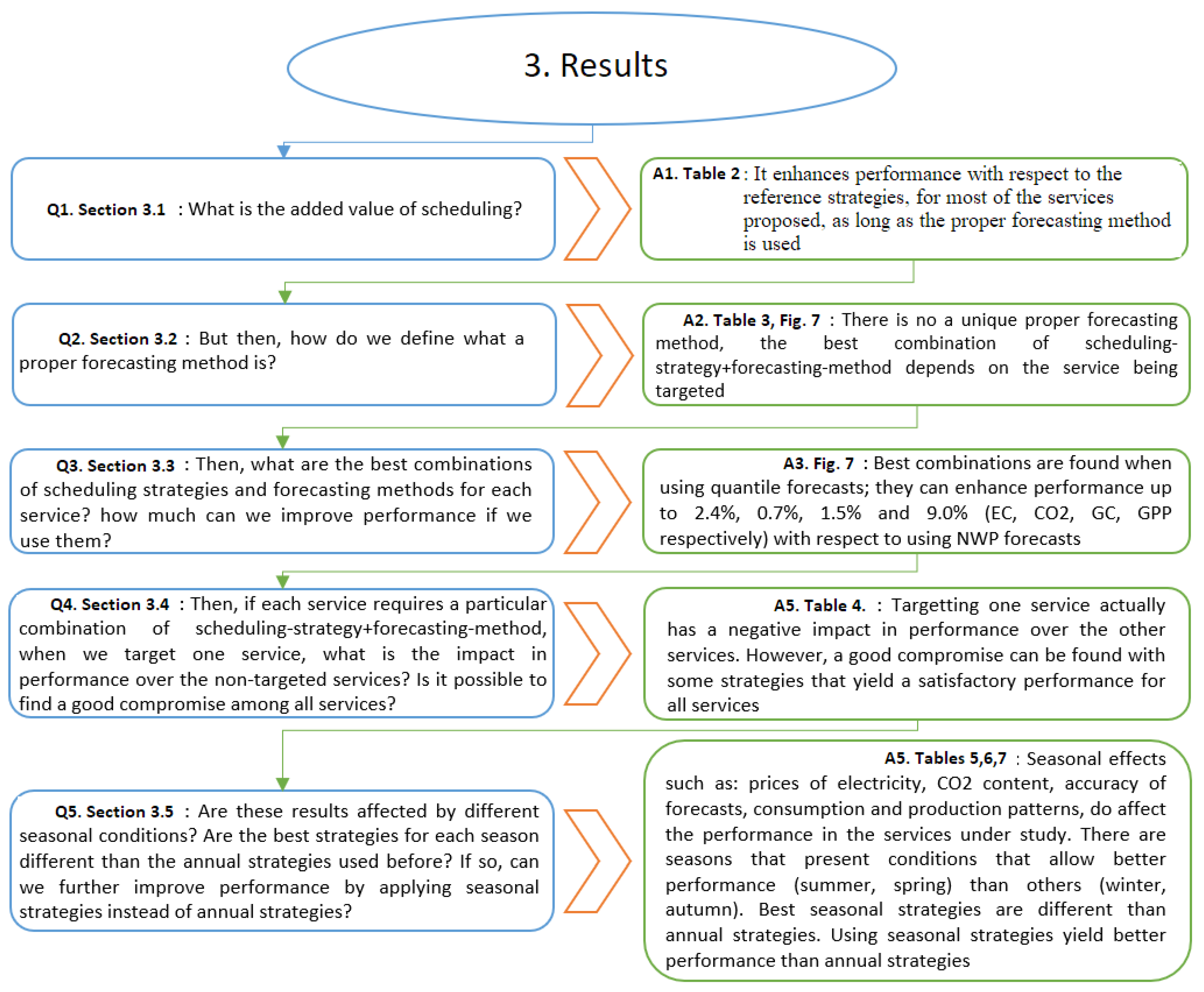
The first EMS strategy that is envisaged to be implemented in the Drahi-X smart-building is a basic rule-based balancing-strategy, designated as P V B m a x . This strategy privileges the use of all the available PV potential (self-consumption) and the battery. Similar variations of this strategy are also commonly used in low-power commercial PV charge controllers, which adds to the interest of using it as a reference strategy. However, the main interest of using this strategy as a benchmark is to observe whether the proposed EMS strategies could bring an improvement in performance regarding the services being evaluated. This strategy, even when conceived as a balancing strategy, can also perform scheduling if a forecast of the PV production is given. Therefore, we use this as a reference strategy for both balancing only ( P V B m a x ) and scheduling ( P V B m a x N W P ). Figure 6 presents a flow diagram representing the working principle of the strategy.

3. Results

3.1. Performance of the Proposed Scheduling Strategies

Scheduling can be defined as the planning of the use of resources in a MG, for a given window of time in the future. Therefore, derived from this statement, the first advantage of performing scheduling is the ability to offer some services (such as the grid-commitment that is introduced in this work), which, due to its intrinsic nature, can only be offered if scheduling is performed.
Table 2 summarizes the results in performance of three reference strategies and the three proposed EMS scheduling strategies, regarding the four services under study, denoted by their performance indicators: EC, CO 2 , GPP, and GC. The values in bold represent the best performance that was obtained for each indicator. In this table, a quantile forecast expressed, like: AnEn τ =x1:x2 means that any probability level (i.e., quantile) between x 1 and x 2 produces the same-optimal-performance with the strategy being used.
This cross-comparison against reference strategies is important, as some studies in the field only focus on developing new functionalities or proposing new EMS strategies, without benchmarking against basic reference cases. This is valuable when justifying the necessity or showing the added value of having a MG and/or implementing a novel EMS strategy. The first reference case is when we assume that there is no MG deployed (NO MG in Table 2); therefore, all of the consumption is supplied by the utility grid. The second and third strategies used as reference are the PVBmax balancing strategy and the PVBmax scheduling strategy, that are presented in detail in Section 2.4.2. A summary of the proposed strategies (scheduling and balancing), including the type of algorithm used, the target objective, as well as the reference to the objective function equations (when applicable), is presented in Table 1.
In Table 2, we observe that, with the exception of the CO 2 min strategy, all of the proposed scheduling strategies outperform all the reference strategies in the services they target. The exception with the CO 2 content is comprehensible, as the embedded CO 2 emissions (due to the manufacturing process) of the battery and PV panels are high, when compared with the carbon footprint of the energy coming from the French national grid.
This result shows the importance of developing an EMS strategy that targets the specific service that we want to optimize, as it will most likely obtain a better performance than a strategmey that is not ant to optimize the same service.
In this particular case, the scheduling method proposed proves to bring an added value to the MG in terms of performance, with respect to the strategy that is envisaged to be deployed in the Drahi-X building, as long as the proper forecasting method is chosen. This conclusion brings out a question: what does it mean “a proper forecasting method”? What characteristics define it? The answer to this question is addressed in the following section.

3.2. Optimistic and Pessimistic Forecasts: The Versatility of Quantile Forecasting

At the heart of a scheduling strategy, there is always a PV production forecast. An EMS that performs scheduling of distributed energy resources, for a given window of time in the future, requires forecasts as inputs. But forecasts are never 100% accurate, then, their intrinsic uncertainty becomes an important subject to be studied as presumably, this will have an effect on the final performance obtained from a given scheduling strategy.
Recalling the statistical definition of quantile, what the deterministic quantile forecasts say is: if a given quantile τ with probability level x is used as a prediction (i.e., x f c a s t = τ x ), then there will be x % of probability that the bias (i.e., the forecasting error) is positive, being the bias computed as the difference between the forecast value and observation (i.e., B = x f c a s t x o b s ). This is an interesting characteristic of the quantile forecasting method, as it allows for the decomposition of the bias or forecasting error E f c a s t in two components, namely: the -absolute- magnitude and a the sense or direction. Quantile forecasting allows us to choose (to some extent) between the absolute magnitude and the sense or direction of the forecasting error, which can be beneficial in an application where having a bias in a given direction is more beneficial than having it in the other direction (or not having it at all).
The results are obtained for the entire test period and they are summarized in Table 3. In this table, the GC indicator is also included, as grid-commitment is a common service to all of the scheduling strategies (ECmin, CO 2 min and GPPmin), assured by the balancing module (BAL). Here, we show the results of using a very pessimistic forecast (AnEn τ =0.1; rMBE = −0.354, rMAE = 0.384), a very optimistic forecast (AnEn τ =0.9; rMBE = 0.316, rMAE = 0.329), a quasi-unbiased forecast (PE; rMBE = −0.001, rMAE = 0.372), a low-bias high-accuracy forecast (NWP; rMBE = −0.002, rMAE = 0.219), and a perfect forecast (PF; rMBE = rMAE = 0).
The best results (bold values) for all indicators are obtained with the perfect forecast (PF), with a 100% of GC for the three scheduling strategies as well as the smallest values for EC, CO 2 , and GPP, as stated in Table 3. This is consequent, as the optimal strategies found during scheduling are being strictly followed when a perfect forecast is used (the most accurate forecast possible), hence the optimal performance is achieved. However, this scenario is unrealistic, as having a perfect PV-power forecast is most likely unachievable.
Regarding the ECmin strategy, we observe some correlation with the bias of the forecasting error, as EC presents its highest (worst) value with the most pessimistic forecast (AnEn τ =0.1), followed by the most optimistic forecast (AnEn τ =0.9) and the persistence forecast (PE), which has low-bias and high-absolute-error. This suggests that this service requires low-bias and low-absolute-error forecasts to yield the best performance, as is the case when using the NWP and PF. The difference between the best and the worst strategies (ECmin-PF and ECmin-AnEn τ =0.1 respectively) are as high as 92.8%, which represent an increase in the price of the electricity of 0.14 €/kWh. However, it must be remarked that the smallest cost obtained (using ECmin-PF) is approximately 0.154 €/kWh, which is competitive with the tempo tariff only in the peak hours of the white and red days, where the electricity price is higher than this value. This remarks the importance of optimally deciding when to store/use energy from the battery, and when is better to buy the energy directly from the utility grid, in order to optimize this service.
Regarding the CO 2 indicator, the highest value is obtained with the most optimistic forecast (AnEn τ =0.9) forecast, which is 41.2% higher than the reference PF case, followed by the AnEn τ =0.1 approach (+15.9%), the persistence approach (+3.2%) closing with the NWP forecasting method that only presents an increase of +1.6% with respect to the reference PF approach. There is a clear difference here between the results of the quantile forecasts (AnEn τ =0.1, AnEn τ =0.9) and the other two forecasting methods (PE, NWP), which suggests that this service is favored by low-bias forecasts.
The carbon footprint when using the CO 2 min-PF strategy is 63 gCO2/kWh, which is higher than the mean and mode of the carbon footprint that is associated to the electricity coming from the utility grid. This fact helps to explain the results that were obtained in Table 2, that show that the average CO2 content is higher when a MG is deployed, due to the high embedded CO2 emissions of the battery and the solar panels.
Regarding the GPPmin strategy, the behaviour is a little bit different. In this case, the smallest contracted power (i.e., the best performance) is obtained with the most pessimistic (AnEn τ =0.1), most unbiased (PE), and most accurate (PF) forecasts, at the same time. From this fact, it could be concluded that optimistic forecasts such as AnEn τ =0.9, are not favorable for the grid-peak-power service. The reason behind is the fact that, under-estimative (or unbiased) forecasts, are more likely to have errors that result in battery getting fully charged, hence promoting the PV curtailment. When this happens, the scheduled—smooth—grid profile produced by the GPPmin strategy remains less modified. A similar situation happens when the PF is used, as it does not produce changes to the scheduled grid profile. This is not the case when using the NWP forecasts, as it has a more over-estimative tendency when compared to PE or AnEn τ =0.1. For this indicator, the use of the AnEn τ =0.9 and NWP forecasts, leads to an increase of 9.8% in the annual fee.
A similar phenomena occur with the grid-commitment for the three scheduling strategies, where the AnEn τ =0.1 forecast, being the most pessimistic, presents the best results. This aligns with the fact that under-estimative (i.e., pessimistic) PV power forecasts, favor the grid-commitment service. The latter throws an interesting conclusion regarding the effect of forecasts accuracy: highly optimistic or pessimistic forecasts (such as AnEn τ =0.9 or AnEn τ =0.1), do affect negatively the performance in some services like EC or CO2 content, that seem to be rather favored by low-bias forecasts (e.g., PE or NWP). On the other hand, a service, like grid-commitment, is favored by pessimistic forecasts, while the grid contracted power, while not presenting a clearly defined behaviour, is less affected when pessimistic forecasts are used.
With the previous results in mind, an EMS is able to favor some services by using different forecasting approaches with errors ranging from under-estimative to over-estimative. This suggests that it does not exist an unique proper forecasting method as such, as it is dependent on the service being targeted. Therefore, if the most suitable forecasts are used for each service, how well can the EMS perform? To what extent can we improve performance in the services proposed? We try to find the answer to this question in the next section
The results shown so far suggest that there are services that benefit from over or under estimative forecasts. Therefore, at the view of this results and acknowledging the fact that a forecasting error will be always present, a proper forecasting method could be defined as such that, due to its persistent under or over estimative nature, allows for the EMS to produce optimal performance in a particular service by providing certainty on the sign of the imbalance between production and consumption.
In the following section, we search for the optimal quantile forecast that must be used in order to optimize the different services.

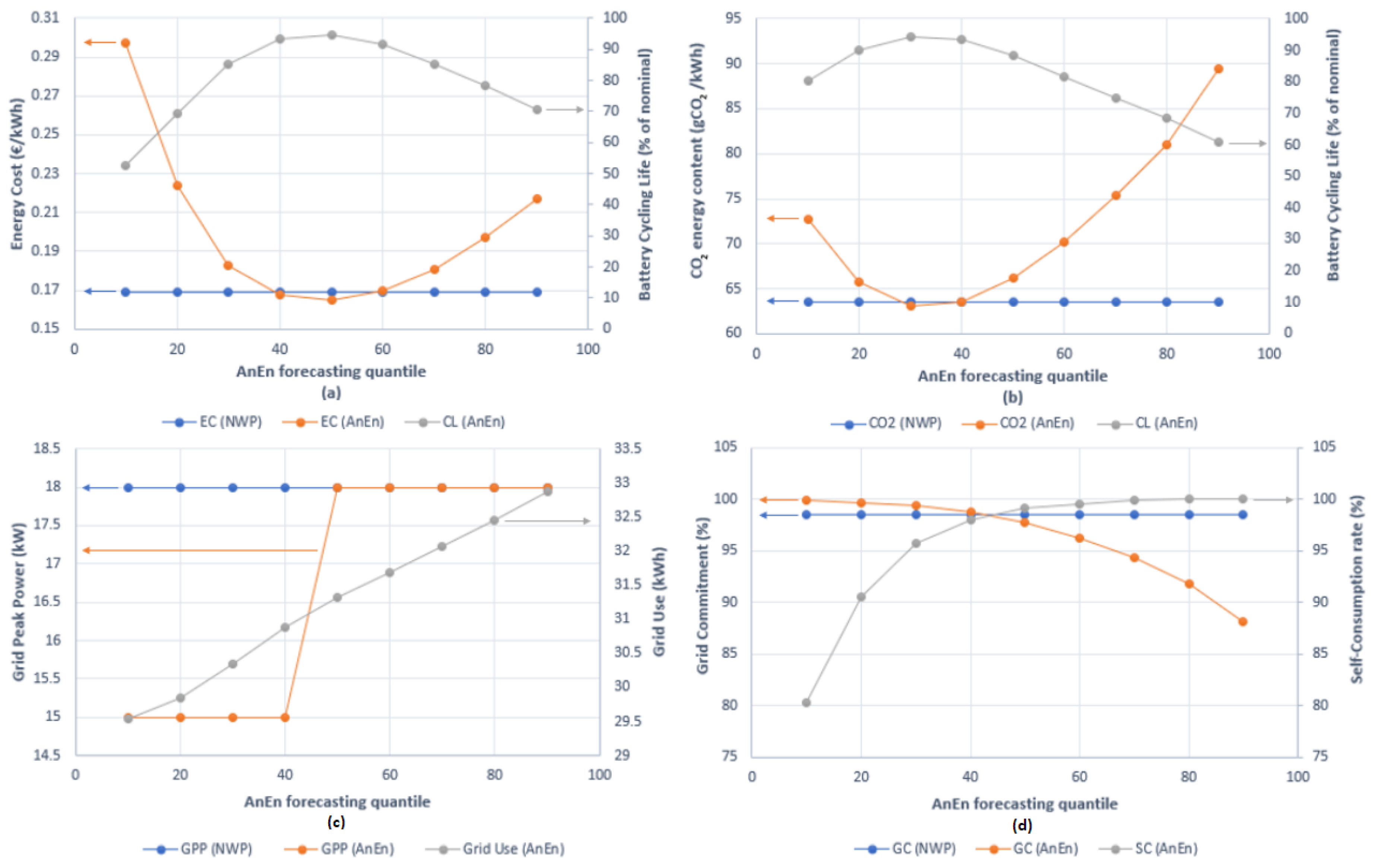
3.3. Optimizing the Services: Finding the Best-Suited Quantile Forecasts

It must be recalled that an optimization-based EMS, such as the ones that are proposed in this work, require deterministic forecasts of PV production. Therefore, quantile forecasts are a way to provide the EMS with a deterministic forecast that has intrinsic probabilistic information embedded. More specifically, the most valuable information that we can extract from a quantile forecast is the probability of the error being either over or under estimative. By knowing this information in advance, we can deliberately use the forecasts that are best suited for the service being targeted during the scheduling.
The results that are presented in Figure 7 include the PV costs, reduction in the expected Through-Output-Energy (TOE) of the PV array due to curtailment, as well as the correction in battery cycling life. The TOE is the total energy that is expected to be delivered by an element (i.e., PV panels, battery) throughout its working lifetime in an specific place. In other words, the electricity cost and CO2 content for the battery and PV energy is affected by the profile of use, following Equations (A3), (A6), (A9), and (A10).
The results that are shown in Figure 7a are obtained with the ECmin scheduling strategy, while the ones of Figure 7b are obtained with the CO 2 min scheduling strategy. In both plots, the battery life is presented as a gray curve that represents the battery cycling life as a percentage of the nominal cycling life (i.e., the maximum possible cycling life).
In both cases, the reduction in battery life plays a major role in the behaviour of both EC and CO 2 indicators, as they find its minimum value, where the battery life is maximum. In both cases, the quantile forecasts permit obtaining a better performance (however marginal) than NWP, being EC and CO 2 2.4% and 0.7% less than the values that were obtained using NWP, respectively. It is important to remark than the best performance for the EC is obtained while using the AnEn τ =0.5 forecast, while the lowest carbon footprint is found using the AnEn τ =0.3 quantile forecast. This is important because it remarks the fact that the most accurate forecast (i.e., the one presenting the smallest rMAE or rRMSE) does not always yield the best performance in every service.
Regarding the minimization of the contracted power that was observed in Figure 7c, quantiles forecasts below AnEn τ =0.4 allow for a reduction of 16.6% with respect to the NWP forecasts. Above AnEn τ =0.5, the performance is the same for both quantile forecasts and NWP, which allow a contracted power of 18 kW, according to the tempo tariff. This fact can be explained as for higher quantiles there is over-estimation of the PV production, which would lead to a situation where the system will empty the battery and make use of the grid in order to compensate for the over-estimations of PV production.
If we look at the grid-commitment in Figure 7d (GC-orange curve), it presents a pseudo-parabolic decrease with the increase of the quantile. In contrast, we observe that the self-consumption (SC-gray curve) increases, also following a pseudo-parabolic pattern. This can be simply explained, as follows: over-estimative forecasts (i.e., high quantiles) provoke errors that have to be counteracted by the grid, as it foresees more PV production than the actual. Therefore, all of the PV power available is used (SC = 100%), but the grid deviates from its scheduled profile in order to compensate the errors (which implies lower GC). On the other hand, for under-estimative forecasts (i.e., low quantile forecasts), there will be excess of PV power that is counteracted by means of PV power curtailment (i.e., lower SC), when the battery gets full. In the latter case, the MG is able to closely follow the scheduled grid power profile, yielding the highest values of GC. The highest performance (GC = 100%) is obtained with the AnEn τ =0.1 quantile forecast (that is, at the same time, the least accurate), and it outperforms NWP by 1.5%.
In this section, we realized the advantage of the quantile forecasts, which give us the flexibility to “choose”, to some extent, the desired direction of the bias (or forecasting error), in order to favor a given service. Using these results, we managed to improve the performance of the services (independently) to a certain extent, and we found the best combinations of scheduling-strategy + forecasting-method for each service (graphically seen in Figure 7). However, given that the best combination of scheduling-strategy + forecasting-method is different for each service, when we chose to optimize one service, what is the impact over the other services? Can we find a strategy that produces a good performance for all services? This question is tackled in the following section.

3.4. Impact in Performance of Targeting One Service over the Non-Target Services

This section explores how performing optimal scheduling targeting a particular service, affect the performance of the non-targeted services. If so, it would be of interest to know in which way and to what extend those other services are affected. In order to answer this question, the best combination of scheduling strategy+forecast, for each one of the services, is run for the test period. As usual, the output of the scheduling module passes through the balancing module before outputing the final power profiles. In this way, the performance of each scheduling strategy regarding its target and not-target services can be cross-compared, in order to see the impact among the different strategies.
All of these results are summarized in Table 4, where the numbers in bold represent the best values that were obtained for each service, and the positive/negative bias represents a relative increase/decrease of the corresponding performance indicator with respect to the best performance obtained for that service. In this table, the percentage with respect to the best result of the GPP indicator represents the percentage-difference in terms of the annual fee that must be paid, depending on the contracted power required, as it was considered to be more meaningful for the purposes of the comparison of this indicator.
There are two main results to take away from this table, with the first one being the fact that the best performance in each service, is obtained when using the scheduling-strategy-plus-forecast that targets that service. This validates the usefulness of the proposed scheduling strategies, as they allow for producing improvements in performance in every service studied. The second interesting fact, and related to the previous one, is that a scheduling strategy always under-performs for those services it does not target. For instance, in the case of EC, the best performance (0.165 €/kWh) is obtained with the ECmin-AnEn τ =0.5 scheduling strategy. Its performance in the other services is always sub-optimal. Regarding CO2, the best performance is obtained with the CO 2 min-AnEn τ =0.3 strategy (63 gCO2/kWh), and the GPPmin-AnEn τ =0.4 yields the best performance in GPP (15 kW). Regarding the grid-commitment, it is not favored by any scheduling module, but by the balancing module, that is present for all of the scheduling strategies. However, based on the results obtained for the test period, it was found that the ECmin-AnEn τ =0.1 combination, produced the best annual performance for this service, among the different strategies.
Another important fact that comes back again in this result is that, in order to obtain the best performance in each service, different (quantile) forecasts must be used (that are not always the ones presenting the smallest absolute errors rMAE, rRMSE). That highlights the importance of the versatility that is provided by use of the quantile forecasts obtained with the AnEn method, which outperform the results obtained with the reference NWP forecasts. Now, it is reasonable to wonder if it is possible to find a strategy that produces a good compromise, in terms of performance, among all services. It is true that, sometimes, the price to pay in order to achieve the best performance in one-target-service is big (regarding the remaining services), and the superiority in the target service can be marginal, with respect to the other strategies. For instance, if we take the ECmin-AnEn τ =0.1 strategy, it yields the best performance for the grid-commitment service, with a value of 99.9%. However, the advantage in the performance of this indicator with respect to the other strategies is not huge, as the worst performer in this indicator is the ECmin-AnEn τ =0.5 strategy, which under-performs by only 1.2%. At the same time, the “price” in terms of performance of the not-targeted services that we have to pay if we want to obtain the best GC performance, is very big (with values up to +66.5% in carbon footprint, +80% regarding EC or −57.4% in GPP). At the view of the above, it might not be worth it to use the ECmin-AnEn τ =0.1 strategy, and rather it would be more beneficial to choose another one that produces a better compromise among all of the services. If we observe the strategy that presents the smallest under-performance values of all, is the GPPmin-AnEn τ =0.4. Accordingly, we could say that this strategy presents the best compromise for all the services, followed by the ECmin-AnEn τ =0.5 strategy.
From this section, we conclude that targeting one service (with its best scheduling-strategy + forecasting-method) affects negatively the performance on the other services (i.e., the best performance of each service is only achieved when the best combination of scheduling-strategy + forecasting-method for that particular service is used). However, a good compromise can be found with some combinations that yield satisfactory performance for all services. At the view of the above we wonder: can these results be affected by different seasonal conditions? How can these best combinations of “scheduling-strategy + forecasting-method” be adapted for each season? Could we further improve the performance by applying seasonal EMS strategies rather than annual strategies? The answers to these queries are tackled in the following section.

3.5. Seasonal Performance Optimization and Analyses

Because every building is exposed to different conditions that have a seasonal behaviour (i.e., different degrees of accuracy of the PV forecasts, different PV production and consumption patterns, different prices of electricity and CO2 content), the last question that arises regarding this analysis is: how much these seasonal effects can affect either positively or negatively the performance of a SB?
In order to answer this question, we take the best EMS strategy (i.e., best combination of scheduling strategy and quantile forecast) based on their performance for each service and for each season of the year. Table 5 presents the summary of these strategies. In this table, when a quantile forecast has two quantiles (e.g., AnEn τ =10:90), it means that any quantile from AnEn τ =0.1 to AnEn τ =0.9 yields the same (optimal) results for that strategy. It is already very interesting to note how, for a given scheduling strategy, the forecasts that produce the best results can be so different between seasons. For instance, if we use the CO 2 min scheduling strategy, we require the AnEn τ =0.1 forecast in autumn to obtain the best results, whereas, in summer or spring, is the AnEn τ =0.4 forecast the one that yields the best performance. In contrast, when using the GPPmin strategy, any quantile forecast will produce the optimal performance in autumn, while is the AnEn τ =0.2 only in winter, which produces the best results. The versatility of using quantile forecasts for energy management is again highlighted here, as it permits customizing an EMS according to a particular service and season of the year, in order to obtain optimal performance. The strategies described in Table 5 are run for each season, and the results are summarized in Table 6. The values in parenthesis represent the percentage difference with respect to case when the same scheduling strategies are run while using the-reference-NWP forecasts.
We observe in these results that most of the scheduling strategies that use quantile forecasts achieved a better performance than the same scheduling strategies using NWP forecasts. The exception is the GPP during spring, summer and autumn, where there is no improvement, and the carbon footprint in summer that presented a marginal increase when using quantile forecasts. Even when some of the improvements are marginal, there are some others that are significant, such as the carbon footprint in autumn, which decreased 24.1% or the GPP in winter that decreased 16.7% when using quantile forecasts instead of NWP. This supports the added value of using quantile forecasts in energy management to obtain better performance by customizing the EMS strategy to different operating conditions and requirements.
Regarding the seasonality differences, we see clearly that, with the exception of grid-commitment (that achieved a 100% in all seasons), for the rest of services (i.e., EC, CO 2 and GPP), the performance is always better in summer and spring and the worst during winter and autumn. It must be recalled that several factors play a role in the differences in performance for the different services. Common to all of them, there is the annual variations in the consumption patterns. There is also the annual variability in PV output power (i.e., PV power availability), where the intensity in the PV power available as well as the longer duration of the night during winter months, is a factor that clearly impacts the performance of a system powered by photovoltaic panels.
As mentioned previously, the accuracy of the forecasts also changes throughout the year. Besides the above mentioned aspects (common to all scheduling strategies), ECmin and CO 2 min are affected by the variations of the prices and CO2 content of the electricity coming from the grid. The sum of the effects of all these aspects conditions the response of the different scheduling strategies that try to find a way to achieve their goals under these constraints.
A third question that arises after the results presented so far in this section is whether adopting a seasonal EMS strategy (i.e., using the strategies of Table 5 during the corresponding season) produces better results, by the end of the test period, than using a unique EMS strategy for each service (i.e., EMS strategies of Table 4) during the entire test period. The values in parenthesis of the seasonal strategies represent their percentage performance with respect to the case when the best annual-strategy for each service is used.
The results are summarized in Table 7, where we can observe that, for the grid-commitment, the seasonal strategy presents only a marginal improvement of 0.1% over the annual strategy. Similarly, for the grid-peak-power there is no difference between both approaches. On the other hand, we have a marginal decrease of 0.5% in the CO2 content for the seasonal strategy respect to the annual strategy, whereas the energy-cost experience a more significant reduction of 9.1% if the seasonal strategy is used. We can conclude then that the seasonal strategy presents an overall better performance with respect to the annual strategy. At the view of the results that are presented in Table 5, where it is clearly stated that, for the different seasons of the year, different forecasting methods should be used in order to obtain the optimal performance. Therefore, an annual strategy, that makes use of a single forecast throughout the test period, is expected to under-perform a seasonal strategy.
We can then conclude that seasonal effects, such as: prices of electricity, carbon footprint, accuracy of forecasts, consumption, and production patterns, do affect the performance in the services under study. There are seasons that present conditions that allow better performance (summer, spring) than others (winter, autumn). Best seasonal strategies are different than annual strategies and we proved that using seasonal strategies yield better performance than using annual strategies in some services such as the energy-cost, while, for other services, it is indifferent (e.g., GPP). A flow diagram that depicts the logic followed in this section in order to tackle the different research questions that wanted to be explored along with references to the figures or tables where the answers are found, is presented in Figure 8.

4. Conclusions

A new framework methodology for energy management in smart-buildings that are equipped with a photovoltaic plant and a battery storage system has been presented.
Four services that are related with economical and environmental aspects are used to evaluate performance that target not only the microgrid users, but also the distribution system operator.
A novel service in the domain of microgrids, the grid commitment. Its purpose is to turn a microgrid into a deterministic prosumption (i.e., production-consumption) unit, to the view of the distribution system operator.
The results show that an EMS with optimization-based scheduling strategies, as the ones hereby proposed, is able to outperform the different reference strategies in every service, with improvements of up to 50% in some cases, with the exception of the carbon footprint, where having no microgrid (MG) produces, on average, 4.9% less carbon emissions.
More accurate forecasts (e.g., numerical weather prediction forecasts compared to eccentric quantiles from the analog ensemble method) are seen to result in a better performance, particularly for EC and CO 2 indicators. However, for some services, in particular the grid-commitment and grid-peak-power, and for some optimisation periods, this is not the case. This is particularly palpable in the seasonal analysis, where scheduling strategies using eccentric quantile forecasts outperform numerical weather prediction forecasts (NWP). Improvements in performance of 16.7% for GPP during winter or 24.1% for CO2 emissions during autumn can be obtained.
In an annual-based analysis, quantile forecasts permit obtaining better performance in EC, CO 2 , and GC, in comparison with the deterministic NWP forecasts. However, the improvement is mostly marginal. At the same time, in a seasonal-based analysis, the advantages of using quantile forecasts can be more significant, achieving improvements in performance of 16.7% for GPP during winter or 24.1% for CO2 emissions during autumn, with respect to the base-case NWP forecasts.
The results confirm that the best service indicator is found when the scheduling optimization is oriented for that service, while under-performing in the non-targeted services.
Targeting the grid-commitment is the most expensive decision, as it is the one that affects more negatively the other services. This is due to the massive PV curtailment that is provoked by the use of a very pessimistic forecast (AnEn τ =0.1). Therefore, a good compromise to obtain fairly good performance in all services, is found with the GPPmin-AnEn τ =0.4 strategy, followed by the ECmin-AnEn τ =0.5 strategy.
The seasonal analyses show that the best accuracy of forecasts and performance of EC, CO 2 and GPP is obtained in summer and spring, while the worst performance is obtained in winter and autumn. Winter is particularly the season when the price of the electricity is the highest and solar resource is at its lowest, while autumn is the period when the energy is more loaded with CO2.
As quantile forecasts allow for customising the scheduling optimization for each season of the year, the implementation of a seasonally-adapted EMS strategy might be plausible. However, the results for this study-case demonstrated that a seasonal EMS strategy is only beneficial regarding the energy-cost, where a decrease of up to 9.1% can be achieved.

Author Contributions

F.C.-O.: Main research, results analysis, figures and tables creation and writing of the article. J.B.: Revision and validation of results, funding obtention. A.M.-D., V.B.: Revision of the article. All authors have read and agreed to the published version of the manuscript.

Funding

This action benefited from the support of the Chair-Challenging Technology for Responsible Energy—led by l’X—Ecole polytechnique and the Fondation de l’Ecole polytechnique, sponsored by TOTAL.

Acknowledgments

This work was supported by the Energy4Climate Interdisciplinary Center (E4C) of IP Paris and Ecole des Ponts ParisTech and by the 3rd Programme d’Investissements d’Avenir [ANR-18-EUR-0006-02].

Conflicts of Interest

The authors declare no conflict of interest.The funders had no role in the design of the study; in the collection, analyses, or interpretation of data; in the writing of the manuscript, or in the decision to publish the results.

Appendix A. Nominal and Adjusted Values for Battery and PV Energy

Appendix A.1. Energy Cost Calculations

In this section, the calculations to compute the nominal and adjusted costs of the energy coming from the battery and the PV panels are presented.
The nominal cost for the use of the battery is computed using Equation (A1).
C b a t t n o m = C A P E X b a t t T O E m i n
where C A P E X b a t t stands for the capital expenditure (the cost) of the battery, while the T O E m i n stands for the minimum through output energy of the battery or the minimum energy that the manufacturer guarantees that the battery will deliver during its lifetime (see Table A1). The T O E m i n is computed for specific test conditions set by the manufacturer of the battery.
In our case, we assume that T O E m i n is computed for the nominal battery cycling life C L m a x . Therefore, when CL decreases, that causes T O E to decrease accordingly, increasing the cost of the energy delivered by the battery in the same proportion. The correction factor for the reduction in the battery cycling life B L R , is presented in Equation (A2).
The nominal cost of the energy delivered by the battery C b a t t h , computed in Equation (A1), is adjusted the equivalent cycling life (CL) of the battery [36], as presented in Equation (A2).
B L R = C L C L m a x
where C L is the equivalent battery cycling life while C L m a x is the maximum (theoretical) battery cycling life according to the model proposed by Muenzen et al. [36].
Then, the factor B L R is used to adjust the nominal cost of the battery presented in Equation (A1) to obtain the corrected battery cost. This is expressed in Equation (A3).
C b a t t c o r r = C b a t t n o m B L R
Then, for a given EMS strategy, the equivalent B L R can be computed in order to obtain the corrected battery cost C b a t t c o r r . This cost is considered constant for the entire test period. For the sake of simplicity, we consider that these average use conditions of the battery are kept throughout all its lifetime, so that the reduction of its cycling life is consistent with the calculations.
An analogous approach as the one presented in Equations (A1)–(A3) can be followed to obtain the average cost of PV energy, C p v .
The nominal cost of the energy delivered by the PV panels C p v n o m , can be obtained with the Equation (A4).
C p v n o m = C A P E X p v T O E e x p
where C A P E X p v stands for the capital expenditure (the cost) of the PV array (without taking into account the balance-of-system costs), while T O E e x p represents the expected through-output-energy, which is computed based on the historical PV output power measurements of the study-case site and the warranted life and output-power of the PV panels given by the manufacturer (see Table A1).
In the meantime, an equivalent to the B L R can be found for the PV power production, that is related to the reduction in the through output energy due to curtailment. This is called PV curtailment factor ( P V C F ) and is expressed in Equation (A5).
P V C F = E p v p o t e n t i a l E p v c u r t a i l e d E p v p o t e n t i a l = E p v r e a l E p v p o t e n t i a l
where E p v p o t e n t i a l is the potential output energy of the PV installation during the test period for the given GHI conditions, while the E p v c u r t a i l e d represent the total curtailed energy during the test period.
In this case, for a particular EMS strategy, the results of Equation (A5) are extrapolated as if the curtailment policy were to repeat for the entire life of the PV installation. Under this assumption, Equation (A3) can be rewritten to compute the corrected cost of the energy delivered by the PV panels, as in Equation (A6).
C p v c o r r = C p v n o m P V C F

Appendix A.2. Energy CO2 Content Calculations

Following a similar method as the one presented in Section Appendix A.1., in this section the nominal values for the CO 2 content of the energy delivered by the battery and PV, based on their embedded carbon emissions (see Table A1) are computed.
The nominal values for the CO 2 content of the battery and PV panels are computed as follow:
CO 2 b a t t n o m = E CO 2 b a t t T O E m i n
CO 2 p v n o m = E CO 2 p v T O E e x p
where E CO 2 X stands for the embedded CO 2 emissions expelled to the atmosphere during the manufacturing process of the DER X (see Table A1).
The corresponding corrected values for the CO 2 content of battery CO 2 b a t t h and PV energy CO 2 p v h , are computed by changing the capital cost C A P E X x in Equations (A3) and (A6), and replacing it with the embedded CO 2 emissions during manufacturing. In these way, we obtain the relations to compute the corrected values for the CO 2 content of battery and PV energy, as presented in Equations (A9) and (A10).
CO 2 b a t t c o r r = E CO 2 b a t t T O E m i n · C L C L m a x = CO 2 b a t t n o m B L R
CO 2 p v c o r r = E CO 2 p v T O E e x p · E p v p o t e n t i a l E p v c u r t a i l e d E p v p o t e n t i a l = CO 2 p v n o m P V C F
The coefficients B L R and P V C F are the same as for the calculations of EC (see Equations (A2) and (A5)), as well as the T O E m i n and T O E e x p (see Table A1).
A summary of the C A P E X and embedded CO 2 emissions of the battery and PV panels, as well as their nominal energy cost, is presented in Table A1. The costs do not include balance-of-system expenses.
In order to compute the through-Output-Energy ( T O E ), the expected annual PV production is obtained for the study-case site. This calculation is based upon historical GHI measurements during the test period (≈1 year). This annual energy output is then extrapolated for the number of years that PV panels are expected to last, according to the manufacturer (30 years with a 0.26% annual degradation). In this way, the -average- total energy that the PV array is expected to deliver throughout its lifetime ( T O E ) is obtained.
Regarding the T O E value for the battery, it is the minimum—warranted—energy that the battery will deliver during its lifetime, regardless of its profile of use, according to the manufacturer.
The CAPEX costs are based on—average—market prices in Europe for PV panels and Lithium-ion batteries, for the capacity requirements of the Drahi-X MG.
Regarding the embedded CO 2 emissions (greenhouse gases emitted through the manufacturing process, including extraction of raw materials), several studies were consulted and the values were taken from the ones that seemed more adapted to the European case, and to the manufacturing sites of the type of PV panels and batteries expected to be used in the Drahi-X MG. The references used to obtain the T O E , CAPEX and embedded CO 2 emissions ( E CO 2 ) are presented in Table A1.
With the aforementioned values, Table A1 is completed using Equations (A7) and (A8) to obtain the nominal values of CO 2 content per kWh of energy delivered by the battery and PV panels, respectively. In a similar manner, Equations (A1) and (A4) are used to obtain the nominal cost per kWh delivered by the battery and PV panels, respectively.
Table A1. Nominal cost and CO 2 per kW/h of energy delivered by the battery and PV panels.
TOE (kWh)CAPEX (€) E CO 2 ( kgCO 2 eq ) CO 2 nom ( gCO 2 eq / kWh ) C nom (€/kWh)
PV (16 kWp)581,000 [31]9265 [37]19,520 [38]330.016
Battery (32 kWh)98,100 [39]20,208 [39]2300 [40]230.210

Appendix B. Optimization Algorithms

In this section a description of the optimization algorithms used for the scheduling stage of the EMS as well as the formulation of the objective functions are presented. A genetic algorithm is used to optimize the energy cost (EC) and the CO 2 content (CO2). The flow diagram that describes its working principle is shown in Figure A1 and the hyper-parameters obtained after tuning the algorithm are presented in Table A2.
Figure A1. Flow diagram of the genetic algorithm method.
Energies 13 05882 g0a1
Table A2. Summary of the penalization weights and hyper-parameters chosen for the Genetic Algorithm formulation.
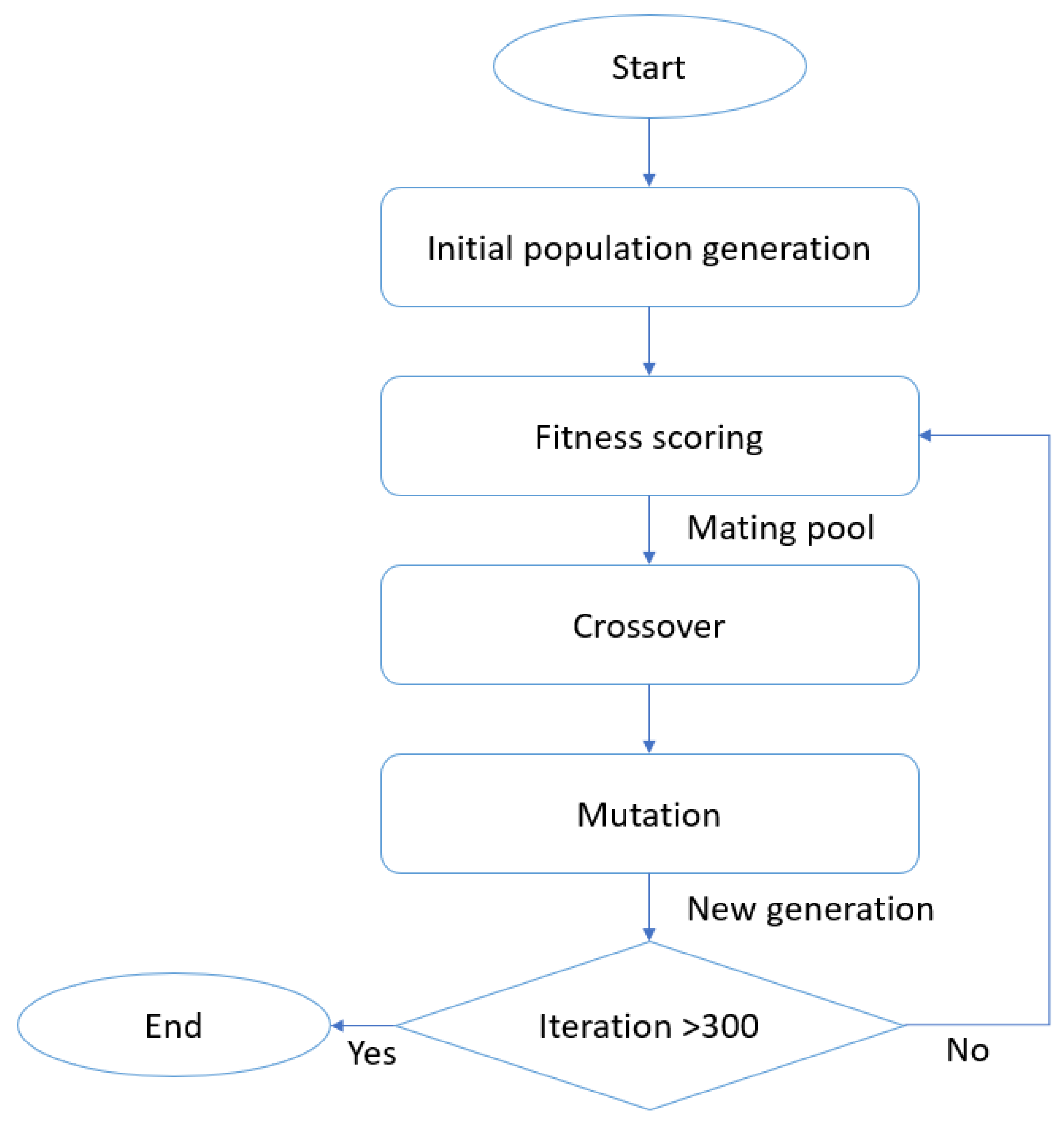
Penalization Weights
K1 × 10 6
L5
M1 × 10 5
Hyper-Parameters
# of Iterations300
Population size1000
Mutation probability100%
# of mutating chromosomes1
Mating pool size (# of parents)100

Appendix B.1. Energy Cost Minimization

The energy cost E C , is the first service minimized using the genetic the GA. The costs of the battery and PV energy, included in the objective function (see Equation (A11)), correspond to the constant non-corrected nominal values C n o m , presented in Table A1. The correction due to battery-life reduction and PV curtailment, expressed in Equations (A3) and (A6), is computed once the grid power profile for the entire test period has been generated. This has to be this way since, as expressed in Equations (A2) and (A5), a prior grid profile is required to compute the correction factors B L R and P V C F . The optimization problem, including the objective function and its constraints, is expressed in the set of Equations (A11).
P b a t t M i n h = 1 24 Δ t · ( P g r i d h · C g r i d h + P b a t t h · C b a t t h + P p v h · C p v h + M · P g r i d h ) + L · S o C d e v + K · S o C o u t w h e r e : C b a t t h = 0 if P b a t t h < 0 C g r i d h = 0 if P g r i d h < 0 M = 0 if P g r i d h > 0 s . t . P g r i d h + P b a t t h + P p v h + P l o a d h = 0 Δ t · h = 1 24 P b a t t h = 0 ( S o C h = 24 = S o C h = 1 ) P p v h = P p v h m p p t 0 % S o C b a t t h 100 % 0 k W P b a t t h 27 k W
where P p v h m p p t is the maximum possible PV power output of hour h (i.e., the power delivered by the maximum power point tracker -mppt- controller). The energy delivered by the PV panels is the product of its average-hourly power and the time resolution ( E p v h = P p v h Δ t ). The factors M, L and K represent respectively the penalizing weights of: the energy sent to the grid ( P g r i d h < 0), the deviation from the desired SoC at the end of the day ( S o C d e v ) and SoC values that go out-of-bounds ( S o C o u t ), for a given battery profile, as previously explained in this section.
It can be observed that the costs of grid and battery energy are zero when these resources consume energy. This is done this way because, in the case of the battery, the T O E m i n given by the manufacturer refers to delivered energy, while in the case of the grid energy, our study-case SB is not paid if energy is sent back to the grid. The optimization is supposed to be performed once a day (at midnight) when the PV output power forecasts for the next day become available. The SoC of the battery is constrained to be left, by the end of each day, at the same value as it was at the beginning of it, which in this study is set to 50%.

Appendix B.2. CO2 Content Minimization

The second service that can be optimized during the scheduling is the CO 2 content of the energy consumed in the MG. This variable is also minimized using the GA approach, as for the EC. Therefore, the CO 2 content of the energy coming from the grid is considered known beforehand for every hour of the test period. The formulation of the problem is analogous to the one presented in Equation (A11). The complete formulation of the problem is presented in Equation (A12).
P b a t t M i n Δ t · h = 1 24 ( P g r i d h · CO 2 g r i d h + P b a t t h · CO 2 b a t t h + P p v h · CO 2 p v h + M · P g r i d h ) + L · S o C d e v + K · S o C o u t w h e r e : CO 2 b a t t h = 0 if P b a t t h < 0 CO 2 g r i d h = 0 if P g r i d h < 0 M = 0 if P g r i d h > 0 s . t . P g r i d h + P b a t t h + P p v h + P l o a d h = 0 Δ t · h = 1 24 P b a t t h = 0 ( S o C h = 24 = S o C h = 1 ) P p v h = P p v h m p p t 0 % S o C b a t t h 100 % 0 k W P b a t t h 27 k W
where CO 2 content of the battery and PV energy included in the objective function, correspond to the constant non-corrected nominal values CO 2 n o m , presented in Table A1. The correction due to battery-life reduction and PV curtailment, expressed in Equations (A9) and (A10), is computed once the grid power profile for the entire test period has been generated, for the same reasons exposed for the EC minimization. The factors M, L and K represent respectively the penalizing weights of: the energy sent to the grid ( P g r i d h < 0), the deviation from the desired SoC at the end of the day ( S o C d e v ) and SoC values that go out-of-bounds ( S o C o u t ), for a given battery profile, as previously explained in this section.

Appendix B.3. Grid Peak-Power Minimization

The third service that was envisaged to be optimized by the scheduling module was the required contracted power or grid-peak-power (GPP). Due to the nature of its objective function, a typical quadratic programming formulation sufficed to solve the optimization problem. The simple formulation, convergence speed, as well as its ability to find true optimal solutions, made us prefer this method over the GA to optimize this service. The minimization of the GPP hereby proposed, falls into the category of quadratic programming problems. Quadratic programming is the process of solving a linearly constrained, quadratic optimization problem, that is, the problem of optimizing (minimizing or maximizing) a quadratic function of several variables subject to linear constraints on these variables. Quadratic programming is a particular type of non-linear programming [41]. The formulation of the optimization problem is presented in Equation (A13). We observe that the same physical constraints as for the GA formulation are present in this problem (see Equations (A11) and (A12)).
P g r i d , P b a t t M i n i m i z e h = 1 24 ( P g r i d h 2 + P b a t t h 2 ) s . t . P g r i d h + P b a t t h + P p v h + P l o a d h = 0 Δ t · h = 1 24 P b a t t h = 0 ( S o C h = 24 = S o C h = 1 ) P p v h = P p v h m p p t 0 % S o C b a t t h 100 % 0 k W P g r i d h 36 k W 0 k W P b a t t h 27 k W
We can note that here there are no costs associated to the power values, as the algorithm is only meant to minimize the peaks of power themselves, trying to make the profile as smooth as possible.
As deduced from its objective function, the method minimizes the power peaks of the grid and the battery simultaneously, reducing not only the required contracted power, but also the depth-of-discharge of the battery, that can lead to extended battery life. There is no associated costs to the grid or battery power, as the power profile itself suffices for the optimizer to obtain the required results. As for the EC and CO 2 , once the algorithm generates the resulting grid and battery profiles for the entire test period, all the performance indicators can be computed and the grid profile is used as the input for the balancing module.
Contrary to heuristic methods such as the GA, quadratic programming methods do not required the tuning of hyper-parameters, which diminish the setting-up time and the uncertainty of obtaining sub-optimal solutions.

References

  1. Zia, M.F.; Elbouchikhi, E.; Benbouzid, M. Microgrids energy management systems: A critical review on methods, solutions, and prospects. Appl. Energy 2018, 222, 1033–1055. [Google Scholar] [CrossRef]
  2. Minchala-Avila, L.I.; Garza-Castañón, L.E.; Vargas-Martínez, A.; Zhang, Y. A Review of Optimal Control Techniques Applied to the Energy Management and Control of Microgrids. Procedia Comput. Sci. 2015, 52, 780–787. [Google Scholar] [CrossRef] [Green Version]
  3. Kuznetsova, E.; Li, Y.F.; Ruiz, C.; Zio, E.; Ault, G.; Bell, K. Reinforcement learning for microgrid energy management. Energy 2013, 59, 133–146. [Google Scholar] [CrossRef]
  4. Mbuwir, B.V.; Ruelens, F.; Spiessens, F.; Deconinck, G. Battery Energy Management in a Microgrid Using Batch Reinforcement Learning. Energies 2017, 10, 1846. [Google Scholar] [CrossRef] [Green Version]
  5. Zhang, D.; Han, X.; Deng, C. Review on the research and practice of deep learning and reinforcement learning in smart grids. CSEE J. Power Energy Syst. 2018, 4, 362–370. [Google Scholar] [CrossRef]
  6. Reynolds, J.; Ahmad, M.W.; Rezgui, Y.; Hippolyte, J.L. Operational supply and demand optimisation of a multi-vector district energy system using artificial neural networks and a genetic algorithm. Appl. Energy 2019, 235, 699–713. [Google Scholar] [CrossRef]
  7. Chaouachi, A.; Kamel, R.M.; Andoulsi, R.; Nagasaka, K. Multiobjective Intelligent Energy Management for a Microgrid. IEEE Trans. Ind. Electron. 2013, 60, 1688–1699. [Google Scholar] [CrossRef]
  8. Herath, A.; Kodituwakku, S.; Dasanayake, D.; Binduhewa, P.; Ekanayake, J.; Samarakoon, K. Comparison of Optimization- and Rule-Based EMS for Domestic PV-Battery Installation with Time-Varying Local SoC Limits. J. Electr. Comput. Eng. 2019, 2019, 1–14. [Google Scholar] [CrossRef]
  9. Ahmad Khan, A.; Naeem, M.; Iqbal, M.; Qaisar, S.; Anpalagan, A. A compendium of optimization objectives, constraints, tools and algorithms for energy management in microgrids. Renew. Sustain. Energy Rev. 2016, 58, 1664–1683. [Google Scholar] [CrossRef]
  10. Khodaei, A.; Bahramirad, S.; Shahidehpour, M. Microgrid Planning Under Uncertainty. IEEE Trans. Power Syst. 2015, 30, 2417–2425. [Google Scholar] [CrossRef]
  11. Li, Z.; Zang, C.; Zeng, P.; Yu, H. Combined Two-Stage Stochastic Programming and Receding Horizon Control Strategy for Microgrid Energy Management Considering Uncertainty. Energies 2016, 9, 499. [Google Scholar] [CrossRef] [Green Version]
  12. Mazzola, S.; Vergara, C.; Astolfi, M.; Li, V.; Perez-Arriaga, I.; Macchi, E. Assessing the value of forecast-based dispatch in the operation of off-grid rural microgrids. Renew. Energy 2017, 108, 116–125. [Google Scholar] [CrossRef]
  13. Sachs, J.; Sawodny, O. A Two-Stage Model Predictive Control Strategy for Economic Diesel-PV-Battery Island Microgrid Operation in Rural Areas. IEEE Trans. Sustain. Energy 2016, 7, 903–913. [Google Scholar] [CrossRef]
  14. Parisio, A.; Wiezorek, C.; Kyntaja, T.; Elo, J.; Johansson, K.H. An MPC-based Energy Management System for multiple residential microgrids. In Proceedings of the 2015 IEEE International Conference on Automation Science and Engineering (CASE), Gothenburg, Sweden, 24–28 August 2015; pp. 7–14. [Google Scholar]
  15. Liu, G.; Xu, Y.; Tomsovic, K. Bidding Strategy for Microgrid in Day-Ahead Market Based on Hybrid Stochastic Robust Optimization. IEEE Trans. Smart Grid 2016, 7, 227–237. [Google Scholar] [CrossRef]
  16. Bogaraj, T.; Kanakaraj, J. Intelligent energy management control for independent microgrid. Sādhanā 2016, 41, 755–769. [Google Scholar] [CrossRef] [Green Version]
  17. Olivares, D.E.; Lara, J.D.; Canizares, C.A.; Kazerani, M. Stochastic-Predictive Energy Management System for Isolated Microgrids. IEEE Trans. Smart Grid 2015, 6, 2681–2693. [Google Scholar] [CrossRef]
  18. Dou, C.X.; An, X.G.; Yue, D. Multi-agent System Based Energy Management Strategies for Microgrid by using Renewable Energy Source and Load Forecasting. Electr. Power Components Syst. 2016, 44, 2059–2072. [Google Scholar] [CrossRef]
  19. Adinolfi, F.; D’Agostino, F.; Massucco, S.; Saviozzi, M.; Silvestro, F. Advanced operational functionalities for a low voltage Microgrid test site. In Proceedings of the 2015 IEEE Power Energy Society General Meeting, Denver, CO, USA, 26–30 July 2015; pp. 1–5. [Google Scholar]
  20. Agüera-Pérez, A.; Palomares-Salas, J.C.; González de la Rosa, J.J.; Florencias-Oliveros, O. Weather forecasts for microgrid energy management: Review, discussion and recommendations. Appl. Energy 2018, 228, 265–278. [Google Scholar] [CrossRef]
  21. Lezama, F.; Soares, J.; Hernandez-Leal, P.; Kaisers, M.; Pinto, T.; Vale, Z. Local Energy Markets: Paving the Path Toward Fully Transactive Energy Systems. IEEE Trans. Power Syst. 2019, 34, 4081–4088. [Google Scholar] [CrossRef] [Green Version]
  22. Hvelplund, F. Renewable energy and the need for local energy markets. Energy 2006, 31, 2293–2302. [Google Scholar] [CrossRef] [Green Version]
  23. Mengelkamp, E.; Notheisen, B.; Beer, C.; Dauer, D.; Weinhardt, C. A blockchain-based smart grid: Towards sustainable local energy markets. Comput. Sci. Res. Dev. 2018, 33, 207–214. [Google Scholar] [CrossRef]
  24. Global Renewables Outlook: Energy Transformation 2050. 2020. Available online: https://www.irena.org/publications/2020/Apr/Global-Renewables-Outlook-2020 (accessed on 3 April 2020).
  25. Tao, L.; Mancarella, P.; Hatziargyriou, N.; Buchhoz, B.; Schwaegerl, C.; Strbac, G. European Roadmap for Microgrids. 2010. Available online: https://www.joinup.ec.europa.eu (accessed on 5 April 2020).
  26. Hatziargyriou, N.D.; Anastasiadis, A.G.; Tsikalakis, A.G.; Vasiljevska, J. Quantification of economic, environmental and operational benefits due to significant penetration of Microgrids in a typical LV and MV Greek network. Eur. Trans. Electr. Power 2011, 21, 1217–1237. [Google Scholar] [CrossRef]
  27. Strbac, G.; Hatziargyriou, N.; Lopes, J.P.; Moreira, C.; Dimeas, A.; Papadaskalopoulos, D. Microgrids: Enhancing the Resilience of the European Megagrid. IEEE Power Energy Mag. 2015, 13, 35–43. [Google Scholar] [CrossRef] [Green Version]
  28. Calderon-Obaldia, F.; Le Gal La Salle, J.; Badosa, J.; Lauret, P.; Migan-Dubois, A.; Bourdin, V. Uncertainty estimation for deterministic solar irradiance forecasts based on analogs ensembles. Appl. Energy 2020. under revision. [Google Scholar]
  29. Alessandrini, S.; Delle Monache, L.; Sperati, S.; Cervone, G. An analog ensemble for short-term probabilistic solar power forecast. Appl. Energy 2015, 157, 95–110. [Google Scholar] [CrossRef] [Green Version]
  30. Badosa, J.; Gobet, E.; Grangereau, M.; Kim, D. Day-Ahead Probabilistic Forecast of Solar Irradiance: A Stochastic. Renew. Energy Forecast. Risk Manag. 2018, 254, 73. [Google Scholar]
  31. Haeffelin, M.E.A. SIRTA, a ground-based atmospheric observatory for cloud and aerosol research. Ann. Geophys. 2005, 23, 253–275. [Google Scholar] [CrossRef] [Green Version]
  32. Tarif Tempo EDF: Grille Tarifaire en 2020 et CGV; Library Catalog, 2018; Available online: Prix-elec.com (accessed on 5 April 2020).
  33. Eco2mix CO2; Library Catalog, 2014; Available online: Www.rte-france.com (accessed on 10 April 2020).
  34. Ferruzzi, G.; Cervone, G.; Delle Monache, L.; Graditi, G.; Jacobone, F. Optimal bidding in a Day-Ahead energy market for Micro Grid under uncertainty in renewable energy production. Energy 2016, 106, 194–202. [Google Scholar] [CrossRef]
  35. Mohamed, F.A.; Koivo, H.N. Multiobjective optimization using Mesh Adaptive Direct Search for power dispatch problem of microgrid. Int. J. Electr. Power Energy Syst. 2012, 42, 728–735. [Google Scholar] [CrossRef]
  36. Muenzel, V.; de Hoog, J.; Brazil, M.; Vishwanath, A.; Kalyanaraman, S. A Multi-Factor Battery Cycle Life Prediction Methodology for Optimal Battery Management. In Proceedings of the 2015 ACM Sixth International Conference on Future Energy Systems, Bangalore, India, 14–17 July 2015; pp. 57–66. [Google Scholar] [CrossRef]
  37. Costs and Economics of Electricity from Residential PV Systems in Europe, European Commission Report. 2019. Available online: https://www.europeanenergyinnovation.eu/Articles/Winter-2016/Costs-and-Economics-of-Electricity-from-Residential-PV-Systems-in-Europe (accessed on 4 May 2020).
  38. Yue, D.; You, F.; Darling, S.B. Domestic and overseas manufacturing scenarios of silicon-based photovoltaics: Life cycle energy and environmental comparative analysis. Sol. Energy 2014, 105, 669–678. [Google Scholar] [CrossRef]
  39. BYD Li-Ion Batteries. 2020. Available online: https://www.mg-solar-shop.com/byd-b-box-l-10.5-battery-storage-10.5-kwh (accessed on 3 April 2020).
  40. Majeau-Bettez, G.; Hawkins, T.R.; Strømman, A.H. Life Cycle Environmental Assessment of Lithium-Ion and Nickel Metal Hydride Batteries for Plug-In Hybrid and Battery Electric Vehicles. Environ. Sci. Technol. 2011, 45, 4548–4554. [Google Scholar] [CrossRef] [PubMed]
  41. Nocedal, J.; Wright, S.J. Numerical Optimization; Springer: New York, NY, USA, 2006. [Google Scholar]
Figure 1. Schematic illustration of the Drahi-X study case microgrid.
Energies 13 05882 g001
Figure 2. Diagram that sketches the working principle of the AnEn (taken from [28]).
Energies 13 05882 g002
Figure 3. Electricité de France (EDF) tempo tariff fee schedule according to contracted power.
Energies 13 05882 g003
Figure 4. Two-stage energy management system (EMS) proposal.
Energies 13 05882 g004
Figure 5. Working principle of the balancing strategy G C m a x . The output of the scheduling module ( P g r i d s c h e d u l e d ), the consumption ( P l o a d ) and the real PV output ( P p v m p p t ) are the inputs of this module.
Energies 13 05882 g005
Figure 6. Flow diagram of the reference P V B m a x strategy. It works as a balancing strategy if real PV-production ( P p v m p p t ) is given, while it performs scheduling if the PV forecasts are provided instead ( P p v f o r e c a s t ).
Energies 13 05882 g006
Figure 7. Impact of probabilistic forecasts in: (a) the energy cost (EC) using the ECmin scheduling strategy; (b) the carbon footprint (CO 2 ) using the CO 2 min scheduling strategy; (c) the grid peak-power (GPP) using the GPPmin strategy and (d) the grid-commitment (GC) and self-consumption rate (SC) using the CO 2 min scheduling strategy. The results include correction for projected battery cycling life reduction (relative to nominal) and PV curtailment.
Energies 13 05882 g007
Figure 8. Flow planning that depicts the main research questions and answers addressed in Section 3.
Energies 13 05882 g008
Table 1. Proposed EMS strategies.
EMS StrategyTypeAlgorithmTarget ObjectiveObjective
Function/Rules
Possible Forecasts
Scheduling
(SCH)
E C m i n Optimization
based
GeneticMinimize
Energy Cost
See Equation (A11)PF (Perfect Forecast)
PE (Persistence)
NWP (Numerical
Weather Prediction)
CO 2 m i n Optimization
based
GeneticMinimize
CO2 content
See Equation (A12)AnEn τ =0.1−AnEn τ =0.9
G P P m i n Optimization
based
Quadratic
Programming
Minimize
Grid Peak Power
See Equation (A13)(Analogs-Ensembles
quantile forecasts)
Balancing
(BAL)
G C m a x Rule basedRulesMaximize Grid
commitment
See Figure 5No forecasts used
Table 2. Performance of the optimization-based scheduling strategies with respect to the reference cases. The best-suited forecasting method for each strategy is used.
Proposed StrategyReference StrategyPerformance
NO MG PVB max PVB max Indicator
EC min -AnEn τ = 0.5 −14.5%−10.3%−8.8% (AnEn τ = 0.1 : 0.2 )EC (€/kWh)
CO 2 min -AnEn τ = 0.3 +3.3%−6.0%−1.6% (AnEn τ = 0.1 ) CO 2 (gCO2/kWh)
GPP min -AnEn τ = 0.4 −36.5%−9.0%−36.5% (AnEn τ = 0.1 : 0.9 )GPP (€)
Table 3. Impact in performance of different types of forecasts.
Scheduling StrategyPerformance IndicatorAnEn τ =0.1
(Pesimistic Forecast)
AnEn τ =0.9
(Optimistic Forecast)
PE
(Unbiased Forecast 1)
NWP
(Reference Forecast)
PF
(Most Accurate Forecast)
E C m i n EC (€/kWh)
GC (%)
0.297
99.9
0.217
92.1
0.176
96.2
0.169
99.1
0.154
100
CO 2 m i n CO 2 (gCO2/kWh)
GC (%)
73
99.9
89
88.1
65
94.3
64
98.5
63
100
G P P m i n GPP (kW)
GC (%)
15
99.7
18
90.8
15
95.3
18
99.1
15
100
1 Aside from the perfect forecast (PF).
Table 4. Impact of targeting one service during the scheduling over the non-targeted services. Quantile forecasts used.
EMS
Intended to:
ECmin-AnEn τ =0.5
Minimize EC
favor GC
CO2min-AnEn τ =0.3
Minimize CO2
favor GC
GPPmin-AnEn τ =0.4
Minimize GPP
favor GC
ECmin-AnEn τ =0.1
Minimize EC
favor GC
Performance indicator % respect % respect % respect % respect
to the best: to the best: to the best: to the best:
EC (€/kWh)0.1650.00.173+4.80.177+7.30.297+80.0
CO2(gCO2/kWh)65+3.3630.064+1.9105+66.5
GPP (kW)30+57.430+57.4150.030+57.4
GC(%)98.7−1.299.4−0.599.3−0.699.90.0
Table 5. Best combinations of scheduling strategy and forecasting method for the different seasons and services.
Performance IndicatorBest Winter EMSBest Spring EMSBest Summer EMSBest Autumn EMS
EC (€/kWh)ECmin-AnEn τ =0.6ECmin-AnEn τ =0.5ECmin-AnEn τ =40:50ECmin-AnEn τ =50:60
CO 2 (gCO2/kWh)CO 2 min-AnEn τ =0.3CO 2 min-AnEn τ =0.4CO 2 min-AnEn τ =0.4CO 2 min-AnEn τ =0.1
GPP (kW)GPPmin-AnEn τ =0.2GPPmin-AnEn τ =0.2:0.3GPPmin-AnEn τ =0.1:0.8GPPmin-AnEn τ =0.1:0.9
GC (%)ECmin-AnEn τ =0.2ECmin-AnEn τ =0.1:0.2ECmin-AnEn τ =0.1ECmin-AnEn τ =0.1
Table 6. Seasonal performance using the strategies of Table 5. Values in parenthesis respresent performance with respect to the performance obtained when using numerical weather prediction forecasts (NWP).
Performance IndicatorWinterSpringSummerAutumn
EC (€/kWh)0.236 (−1.7%)0.114 (−2.6%)0.091 (−5.2%)0.173 (−2.2%)
CO 2 (gCO2/kWh)58 (−2.1%)53 (−0.6%)56 (+1.1%)89 (−24.1%)
GPP (kW)15 (−16.7%)12 (0%)9 (0%)15 (0%)
GC (%)100 (+0.4%)100 (+1.8%)100 (+1.6%)100 (+0.1%)
Table 7. Performance obtained while using a seasonal and an annual energy management strategy.
Performance IndicatorEMS Strategy
SeasonalAnnual
EC (€/kWh)0.150 (−9.1%)0.165
CO 2 (gCO2/kWh)62.8 (−0.5%)63.1
GPP (kW)15 (0%)15
GC (%)100 (+0.1%)99.9
Publisher’s Note: MDPI stays neutral with regard to jurisdictional claims in published maps and institutional affiliations.

