Abstract
This paper describes a control methodology for electronic power converters distributed in low-voltage microgrids and its implementation criteria in general microgrid structures. In addition, a real-time simulation setup is devised, implemented, and discussed to validate the control operation in a benchmark network. Considering these key aspects, it is shown that operational constraints regarding the power delivered by sources, flowing through network branches, and exchanged at the point of connection with the main grid can generally be fulfilled by the presented control approach. The control is performed considering a cost function aiming at optimizing various operation indexes, including distribution losses, current stresses on feeders, voltage deviations. The control system allows an enhanced operation of the microgrid, specifically, it allows dynamic and accurate power flow control enabling the provision of ancillary services to the upstream grid, like the demand–response, by exploiting the available infrastructure and the energy resources. Then, the validation of the approach is reported by using a real-time simulation setup with accurate models of the power electronic converters and related local controllers, of the grid infrastructure, of the power flow controller, and of the communication network used for data exchange. It is also shown that the implemented platform allows to fully reproduce, analyze, and finally validate all the relevant steady-state and dynamic behaviors related in the considered scenario.
1. Introduction
The role of distribution networks in power system management and support is changing dramatically. Revisions of the market framework are expected in the near future in order to exploit distributed resources for supporting upstream medium and high voltage grids [1,2]. In the perspective envisioned by the European directive [3], microgrids will be the bricks of future electric systems. They embrace loads and sources that are close to each other and can be synergized to pursue a safe and cost-effective operation of the electric system and the innovative feature of allowing end-users to become actors of the electricity market. For this aim, microgrids are expected to evolve into systems capable to ensure degrees of scalability, flexibility, reliability, robustness, and readiness similar to networks of digital devices. From the perspective of this analogy, we may refer to E-LAN, namely, Local Area Energy Networks [4]. E-LANs, represented in Figure 1, allow important features, including optimal power flow control, dispatchability at multiple points of connections with the main grid, exploitation of all the energy resources available. In general, advanced control features rely on adequate information and telecommunication (ICT) infrastructures [5]. Such infrastructures are an important constituent of modern intelligent energy systems, whose impact, also in case of malfunctions, is rarely included in studies considering low-voltage distribution grids. Indeed, from the perspective of the required communication protocols and specifications, the considered scenario shows still fluid and evolving [6].
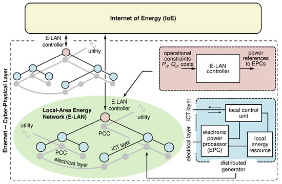
Figure 1.
Modern power system scenario.
Various contributions align along the outlined direction organize microgrid control in multiple layers, as shown in Figure 2. The planning of the resources based on energy arbitrage is found at the higher level of the E-LAN control hierarchy, that is, the transactive control layer, which can be applied both at the microgrid level [1,7,8], also by exploiting detailed mathematical modeling of the distributed energy resources [9], and at the premises of single consumers too [10]. By these approaches, predictions about power needs and energy prices are taken into account to optimally exploit power flow control, as specifically done in [1,8,9]. On the other hand, network models and power flow constraints, which are considered herein, are crucial for optimal utilization of the microgrid distribution infrastructure [11]. This is particularly important when ancillary services, like demand–response, involving additional constraints to be met, have to be accommodated by relying on distributed energy resources interfaced by electronic power converters (EPCs). From this respect, automatic and predetermined power sharing techniques, see, for example, [12], typically constituting the primary control layer of microgrids [13,14], should be augmented to adapt to actual power needs and fulfill given power flow constraints optimally. A contribution from this perspective is given in [4], in which an optimal power flow controller is proposed considering steady-state operation. Herein, the approach is revised and implemented on a real-time simulation platform to evaluate its operation in dynamic conditions. Of course, such approaches may be applied jointly with load prioritization techniques based on load analyses, as proposed in [15]. These techniques can schedule the on/off status of the loads to be supplied by the available sources. The available sources can then be coordinated by optimal power flow control signals. The optimization approach described herein aims at taking advantage of every source available in the grid without using power shedding methods except those enforced at higher levels of the control hierarchy. Instead, enhanced performance of the network is pursued by synergistic use of the control abilities of any distributed power sources.
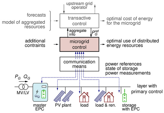
Figure 2.
Local Area Energy Network (E-LAN) control structure.
The validation of the approaches mentioned above is a delicate task due to the complexity and the variety of the dynamics involved (e.g., the fast response of EPCs versus the slow optimization processes and power system dynamics). For these reasons, especially when particularly complex systems are analyzed, validation is often performed by means of computer simulations rather than experimental prototype realizations. Thanks to the recent advances in digital computing, real-time simulators have been employed lately for systems studies involving the interaction of power systems and power electronics systems that are characterized by fast dynamics (e.g., tens of ) [16]. Validation via real-time simulations presents several advantages as compared to traditional simulations. The principal ones are (i) the possibility of performing an on-line testing of models and controls, even while interacting with other hardware components or prototypes [17], and (ii) the possibility of emulating parts of a complex experimental scenario that may not be conveniently included otherwise, due to size, cost, safety, or availability constraints. Several hardware solutions are available to run real-time simulations. Some exploit general purpose toolsets, as shown in [18] and, before, in [19] and [20], others use dedicated hardware and software solutions to ease the development of models of electrical and electronic systems, as done, for example, in [21,22,23].
In this paper, a control architecture that makes use of an innovative optimization framework capable to fulfill the operating constraints while providing synergistic operation of all controllable sources acting in the grid is considered and analyzed. The system performances are optimized in terms of component stress, power sharing, voltage stability, energy efficiency, congestion management, demand–response, robustness against transients, and communication failures. The proposed control is tested by a real-time simulation setup combining real-time simulators (OPAL-RT), industrial central controllers, and communication network emulators. These two aspects constitute the contributions of the paper, that is, (i) describe a power flow optimization method applied dynamically to fulfill power constraints, and (ii) describe the implementation of the proposed power flow control considering a real-time simulation setup integrating fully modeled converters controllers, realistic communication performance, allowing to validate the effectiveness of the proposed optimal control.
In the reminder of the paper, the power flow control is presented in Section 2, while Section 3 presents the primary-local control of the distributed electronic power converters. The implementation of the whole control system is described in Section 4, which also reports and discusses the obtained results. Section 5 concludes the paper.
2. Coordination of Distributed Electronic Power Converters
The power flow control method considered herein is introduced in the following. The method allows to satisfy various operational constraints by exploiting the available distributed EPCs in an optimal way. The method is validated for the first time in this paper by means of real-time simulations and shown suitable for real-time control. The results are reported in Section 4.
2.1. Network Equations
Consider an electrical grid, either single-phase or three-phase, with L branches and N nodes, plus the slack node (node 0) whose voltages are taken as reference voltages. Loads and sources are connected phase-to-phase or phase-to-neutral, while network branches interconnect pairs of nodes. The network graph is described by the incidence matrix , where the column corresponding to node 0 is omitted. For simplicity, but without loss of generality, in the following we will refer to a single-phase network where loads and sources are connected between the grid nodes and a common ground, corresponding to the neutral wire.
Let be the (vector of) node voltage deviations from reference , the currents entering the grid nodes, the voltages across the branches oriented according to the network graph, and the corresponding branch currents. The Kirchhoff’s laws give:
where superscript T denotes transposition. In sinusoidal operation, we represent currents and voltages as phasors and correspondingly we may define the diagonal matrix of branch impedances. Correspondingly, the relations between branch currents and voltages become:
The relations between node voltages and currents are the following:
In (3), is the nodal admittance matrix and its inverse is the nodal impedance matrix. Finally, we get the inverse relations of (1) by:
Remarkably, such equations apply to both meshed and radial networks. In this latter case, .
2.2. Control Equations
Figure 3 schematically represent a network, indicating the kind of nodes and related referred to thereafter. In general terms, the nodes can be classified as:
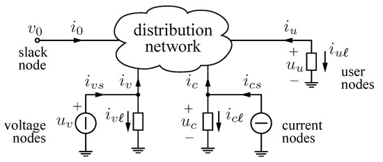
Figure 3.
General network representation.
- (a)
- Voltage nodes, supplied by voltage sources. Let be the voltages imposed at these nodes, referred to the reference voltage . Currents supplied by the sources partially feed local loads () and partially enter the grid ().
- (b)
- Current nodes, supplied by current sources. Currents supplied by the sources partially feed local loads () and partially enter the grid (). Let be the voltages at such nodes.
- (c)
- User nodes, supplying passive loads. Let be the voltages at such nodes and be the related load currents.
The function of balancing the local generation by sources and consumption by possibly connected local loads is in charge of the local controller of the current or voltage nodes. The local controller, depending on the requests coming from the central controller, may adapt its power generation to fully compensate for local load or to pursue local optimization criteria.
It is easy to show that all network voltages and currents can be expressed as a function of voltages and currents impressed by the sources which, in turn, can be controlled by acting on the EPCs interfacing the sources with the grid.
In the following, we therefore consider the voltages impressed at voltage nodes, and the currents entering the grid at current nodes, as the control (input) variables for the entire grid. The main output variables are currents at voltage nodes and voltages at current nodes, all remaining grid quantities being easily derived.
We generally express the control-to-output equations in the form:
where , , , and are sub-matrices of in (3) that refer to voltage and current nodes, respectively, and is the control-to-output transfer matrix.
From the above equations, we express the currents at voltage nodes as:
2.3. Constraints
In general, the grid control problem is twofold. On one side, we wish to optimize some aspects of grid operation, as explained in the following section. On the other side, we need to fulfill specific constraints in terms of power flow at a given set of grid nodes or branches.
More specifically, in order to control the active and reactive power entering the grid at voltage nodes, currents can be constrained. In particular, constraints may apply to their direct (active) and/or quadrature (reactive) terms. Let:
we assume that, among the currents fed by voltage sources, are subject to constraints on the direct component, and are subject to constraints on the quadrature component. Let and be such constrained currents, the constraints are expressed as (superscript ref indicates reference values):
Similar constraints can also apply to the direct and quadrature currents entering the grid at slack node, which are related to the active and reactive power and at the point of coupling with the upstream grid.
Currents fed by current sources can also be subject to constraints, expressed by:
In practice, constraints in (9) reduce the number of control variables, freezing a subset of impressed currents and .
A last type of constraint may impose specific values to a set of branch currents. This corresponds to enforce the power flow in specific grid lines (power steering) or clearing specific branch currents (active insulation). Let be the number of constrained branches, we may express these constraints, separately on d and q axes, as:
2.4. Cost Function
As mentioned before, the E-LAN control variables can be determined according to an optimal control approach, where a suitable cost function is minimized while fulfilling the above set of constraints.
In general terms, we define the cost function as:
where coefficients , , are weighting factors, and variables , , are the cost function terms, defined as follows.
- corresponds to the power loss in the distribution grid, expressed in relative terms as:where is the grid loss in a generic operating condition, is total power loss in the condition when all controllable quantities are set to zero, is the vector of square rms values of branch currents, and is the vector of branch resistances. results by adding (grid loss) and (conversion loss).
- corresponds to the total power loss in the EPCs interfacing the distributed generators with the grid, which can be driven as voltage sources or current sources to implement sources and , respectively. It is expressed by:where is the conversion loss in a generic operating condition, and are the vectors of equivalent series resistances of voltage and current sources, and are vectors of square rms values of source currents.
- corresponds to the cumulative rms deviation of node voltages from voltage reference ; it is given by the ratio between the square cumulative rms voltage deviation in a generic condition and the corresponding value when all controllable variables are set to zero:
It is worth remarking that the coefficients in (11) may be tuned independently in order to assign different weights to voltage deviations, grid losses, and conversion losses on the optimization on the basis of the specific requirements of the application scenario.
In a similar way, we may extend the cost function to include other terms related to the power stress of distributed sources, the thermal stress of feeders, the VA stress of EPCs. The result is a cost function that accounts for the main operation aspects influencing the grid performance, and prevents useless stress of the grid components.
2.5. Solution of the Optimal Control Problem
Eventually, the grid control problem can be formulated as a constrained optimum problem, where cost function is minimized while fulfilling constraints :
where represents the set of constraints expressed in the linear form:
and the cost function is expressed in the quadratic form:
Expressing the matrices shown in (16) and (17) as a function of network quantities, the optimum control problem can solved in explicit form.
It can be observed that the above constraints do not include inequalities. Actually, the quantities that could be constrained by inequalities (e.g., current and power stresses, voltage deviations) are included in the cost function with proper weighting coefficients. The advantage of this approach is that the solution is found in explicit form, thus preventing convergence problems of the solving algorithm and making this latter very fast.
Finally, it is worth remarking that the above approach requires the knowledge of the network topology and network parameters. Actually, even if these data may be not fully available, there are methods presented in literature that allow identification of such information by measurements at grid nodes [24,25,26].
3. Local Control of Electronic Converters
The literature categorizes the behavior of distributed EPCs when taken singularly in grid-feeding, grid-supporting, and grid forming [27]. In the presence of a centralized microgrid controller dispatching optimal power commands to distributed EPCs, the grid-feeding behavior may be convenient, because it allows to easily operate multiple parallel-connected EPCs following given power references, regardless of grid parameters values. Instead, in case of accidental transition to islanded operation, the grid-supporting behavior may be the most favorable, because it allows sustaining the voltage of the local sub-grid section became isolated. This is often done by means of hierarchical structures, as described, for example, in [28], which, typically, aim at defining the operating voltage and frequency of the microgrid, but without specific load sharing schemes based on the available resources and network structure. The control structure in Figure 4, firstly presented in [29], combines valuable merits of grid-following and grid-supporting: it achieves output power regulation when the grid voltage if stiff and supports the grid voltage during transients and in case of transitions to the islanded operation.
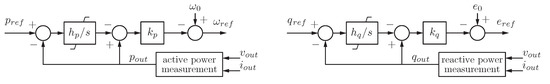
Figure 4.
Droop control scheme with additional power control loop.
Specifically, Figure 5 shows the complete structure of an EPC equipped with inner current and voltage controllers and P-f and Q-V droop loops. On top of these standard control loops, a power regulator with constrained output is employed. The two power control loops, that is, for the active and reactive powers, modify the droop characteristics by vertical shifts in order to make the converter follow given power references. In case of abnormal grid conditions that occur, for example, if the grid becomes particularly weak or islanded, the power controllers tend to saturate automatically. In this condition, the EPCs behave as traditional droop controlled converters, sharing incremental power needs in inverse proportion to their droop coefficients [27].
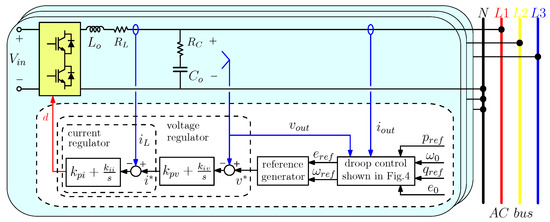
Figure 5.
Control loops of distributed EPCs. comprising an inner inductor current control loop, voltage control loop, and droop laws.
Remarkably, the considered control attains output power flow control while operating connected to the main grid, and autonomous operation with load sharing in case islanded operation occurs.
4. Real-Time Simulation Results
The real-time simulation setup shown in Figure 6 has been implemented in order to evaluate the proposed approaches in steady-state and dynamic conditions. To this end, the benchmark low-voltage network proposed in [30] and arranged as indicated in Figure 7 is considered. Figure 8 displays its model on the real-time simulator.
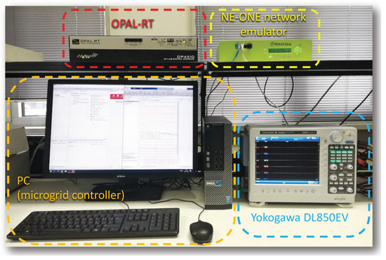
Figure 6.
Real-time experimental setup with highlighted the OP4510 real-time simulator executing the network model and the EPCs control algorithms, the NE-ONE communication network emulator, the PC executing the microgrid controller, and the Yokogawa DL850EV for long-term data acquisition, processing, visualization, and recording.
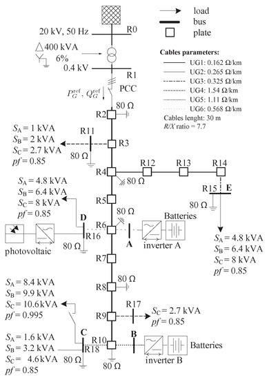
Figure 7.
Considered low-voltage microgrid.
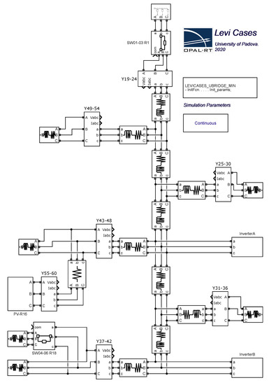
Figure 8.
Network model executed in FPGA.
The setup is composed of an OPAL OP4510 real-time simulator to execute the network model and the EPCs control algorithms, an iTrinegy NE-ONE network emulator to emulate the features of a real communication network, a computer to execute the microgrid controller, and the Yokogawa DL850EV for long-term data acquisition, processing, visualization, and recording. The network and the EPCs hardware are implemented using the eHS Gen 4 Solver and executed, with a time-step of , on the Xilinx FPGA board Kintex-7 325T embedded in the OP4510. EPC controls and communication interface are implemented using Simulink blocks and they executed, with a time-step of , on the four cores of the - Intel Xeon CPU embedded in the OP4510. Such a model partitioning allows performing accurate real-time simulations of the considered network and of the EPC’s hardware on FPGA and, concurrently, execute more complex converters controllers on CPU. The microgrid controller for optimal power flow control is implemented in Matlab and executed, with execution frequency of , on the desktop computer. The performances of the used computer are reported by means of the vector returned by the Matlab command bench: . Control settings and monitoring is allowed by a dedicated graphical user interface, displayed in Figure 9. The microgrid model that is emulated by the OP4510 and the power flow controller that is executed on the computer exchange information representing power-terms by UDP communication via the network emulator NE-ONE. The network emulator can reproduce ideal or impaired communication conditions by including delays, packet loss or corruption, latencies, etc., which allows validation with realistic communication network performances. Finally, data acquisition, visualization, and storage are performed by the DL850EV. This latter is also exploited for active and reactive power measurements using dedicated, embedded processing functions and real-time computation capabilities.
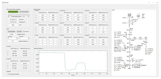
Figure 9.
Graphical user interface for monitoring and control settings.
4.1. Model Structure Details
Figure 10 displays the whole real-time simulation model. The model is partitioned in two parts, one running on the FPGA, the other on the CPU. The FPGA partition contains the model of all the hardware parts, as shown in Figure 8, namely, the grid network specified in Figure 7 and the output filters of the EPCs hardware specified in Table 1. The CPU partition comprises the following blocks.
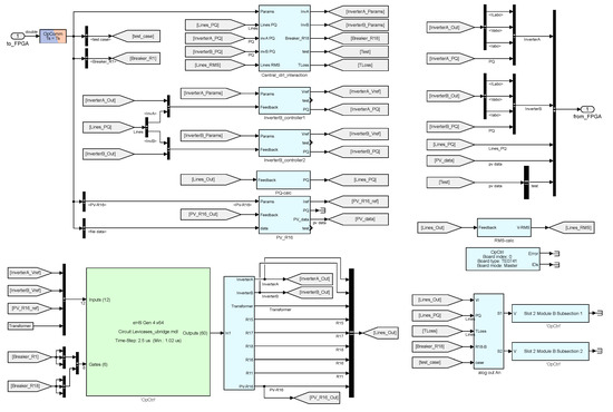

Table 1.
Electronic power processor (EPC) parameters.
- Central_ctr_interaction is responsible for UDP ethernet communication between OP4510 and the microgrid controller running on the computer. The packet rate and control algorithm in execution are ; if needed, this time can be reduced to with computers of higher performance or by dedicated, optimized implementations. This block also (i) logs the results from the running experiment, (ii) acquires and dispatches the control signals that are sent by the microgrid controller to the EPCs, (iii) defines the active power generated by the PV source connected at node R-16 by reading stored data from experimental measurements, and (iv) defines the on/off status of the load breaker at node R-18.
- InverterA_controller and InverterB_controller contain the control loops of the EPCs connected at node R16 and R10, respectively. The control implements the structure shown in Figure 5 and imposes the active and reactive power injection issued by the central microgrid controller and received and dispatched in the real-time simulation by means of the block Central_ctr_interaction.
- PQ-calculator computes the per-phase active and reactive power measured at each node of the network.
- RMS-calculator computes the per-phase rms voltage measured at each node of the network.
- PV_R16 generates the current reference for the PV source on the basis of the power profile generation recorded from a real plant and accessed inside the block Central_ctr_interaction.
- Analog out routes the real-time simulation signals of the model to the analog output ports of the digital simulation platform, whose outputs are then measured by the DL850EV.
The devised partition allows to perform simulation with small discretization steps on FPGA for those models presenting fast dynamics and allow the execution of even complex control algorithm on CPU. The accuracy of the developed real-time simulation setup has been verified by comparison with equivalent desktop computer simulation models executed with variable time step simulations.
4.2. Results
The control system has been tested in different operating conditions. Six scenarios of operation with different kinds of constraints while minimizing the cost function (11) are described next.
- Case 0, no control: the situation in which distributed EPCs are switched off while loads and sources exchange nominal active and reactive powers as defined in Figure 7.
- Case 1, reactive power control: distributed EPCs are controlled by the power flow controller to generate only reactive power in order to minimize the cost (11).
- Case 2, active and reactive power control: as in the previous case, but with active power control too.
- Case 3, power balance at PCC (point of common coupling): distributed EPCs are controlled by the power flow controller to generate the active and reactive power needed to balance among the phases the power absorption at the PCC while keeping the value of the total power exchange at the PCC as in Case 0.
- Case 4, autonomous operation: distributed EPCs are controlled to generate the active and reactive power that is needed to achieve per-phase zero power flow at the PCC, satisfying, in this way, the whole power needs of the microgrid.
- Case 5, demand–response at PCC: distributed EPCs are controlled to generate the active and reactive power to achieve balanced and purely active power flow at the PCC. The active power reference is set to .
The obtained results in steady-state conditions are reported in Table 2, while transient behaviors in relevant conditions are displayed in Figure 11. As a general remark, it is possible to note that voltage deviations and distribution loss significantly reduce in all the considered test cases when distributed EPCs are active and controlled by the microgrid controller. Each operating condition is considered in more details in the following.
Table 2.
Simulation results.
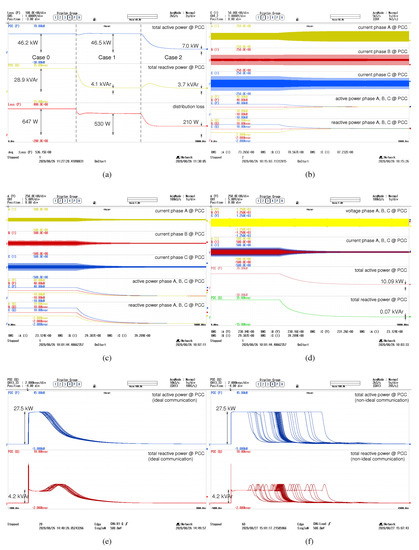
Figure 11.
Results in the considered operating conditions. (a) Distribution losses in Case 0, Case 1, and Case 2; (b) active and reactive power balancing at the PCC (point of common coupling) in Case 3; (c) zero active and reactive power reference at the PCC in Case 4; (d) demand–response at the PCC with requested active power equal to and zero reactive power in Case 5; (e) disturbance rejection at the PCC after a load change within the grid with ideal communication; (f) as in the previous case but with non-ideal communication.
Figure 11a refers to the transition from Case 0 to Case 1 and then to Case 2. It displays, from top to bottom, the total active and reactive power exchanged at the PCC and the measured total distribution losses. Case 1 allows a significant improvement in terms of power quality, indeed the maximum voltage deviation of the network nodes halves and the power factor at the PCC increases from to . In addition, distribution loss is mitigated by . Significant improvements are obtained by activating active power control too: in this case distribution loss decreases by an additional in the last time interval of Figure 11a.
Figure 11b refers to Case 3, reporting the currents through the three phases at the PCC and the correspondingly measured active and reactive powers. Noticeably, power balance is achieved accurately, being the active and reactive powers among the phases at the PCC are of equal amount.
The dynamics related to power flow control are important when considering demand–response at the point of connection with the main grid, which is demonstrated in Figure 11c,d. The former relates to a constraint of zero active and reactive power exchange, the latter to a constraint of pure, balanced active power exchanged with the main grid. Additionally in this case, the optimal coordination of distributed EPCs allows to accurately track the given references.
The impact on the dynamic performances of including communication impairments in the system is considered too in the validation. Figure 11e–f show the effect seen at the PCC after a sudden increase of power absorption by due to the connection of the load at node R18. During the condition in which the control system is set to impose zero power flow at PCC, Figure 11e refers to the case of ideal communication whilst Figure 11f refers to non-ideal and impaired communication with packet loss and random latency in the interval [, ]. Considering the random nature of the considered aspect, a batch of sixty consecutive acquisitions are simultaneously reported in the figures. Figure 11e shows that the control brings back to zero the controlled quantity in a time compatible with the chosen control frequency of if the communication is ideal. Instead, in the case of Figure 11e, dynamics are significantly delayed even though steady-state performance is preserved. Such kind of considerations are important in the design of master–slave microgrid architectures (see, e.g., [31,32]) where a single EPC is expected to buffer possible energy unbalances. In such a case, Figure 11e indicates that a master EPC should be able to buffer about , while in case of communication fault as in Figure 11e the buffered energy increases to , which corresponds to and , respectively, of the capacity of a super-capacitor energy storage as in [33]. In addition, it is possible to note an oscillation due to the active and reactive coupling of the droop control loop.
Figure 12 shows a long-term simulation over ten hours, in which the distribution loss in case of communication impairments is specifically considered. The simulation comprises variability in load power absorption at node R18, which is periodically switched on and off, and in PV power generation, sampled with a time step of one second, which considers a measured profile during a cloudy day. The simulation is run with ideal as well as non-ideal communication, showing negligible impact of communication impairments on power flow optimization: distribution loss increases from an average of to an average of , which confirms the effectiveness of the approach.
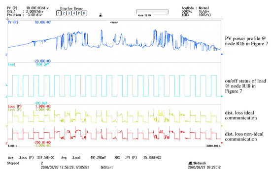
Figure 12.
Long-term simulation (i.e., ) without/with communication impairments.
Finally, Figure 13 shows a long-term simulation over twenty hours in which the load at node R15 is switched on/off randomly, the load at node R18 absorbs the actual power profile measured in a subsection of a university campus, and the source at node R16 generates the actual power profile measured at a PV installation. The figure shows, specifically, the instantaneous distribution loss when the distributed converters are disabled (i.e., case without optimal control) and the case in which the converters are controlled according to the presented optimal power flow (i.e., case with optimal control). Notably, the average distribution loss amounts to in the first case, while, enabling distributed converters to respond to the optimal control signals, the distribution loss decreases to , which corresponds to a distribution loss reduction of .
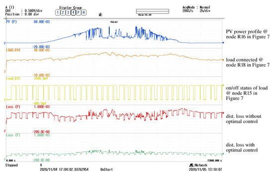
Figure 13.
Long-term simulation (i.e., ) without/with optimal control.
In summary, the described control approach is based on a general algorithm with an explicit solution of the control problem. In this way, it is not affected by convergence issues even in case of communication failures and it is adaptable to generic networks and operating conditions. The approach is validated by means of a real-time simulation setup that is described in detail herein. This setup can be considered for the validation of generic systems involving fast electronic power converters, control algorithms for management of distributed resources, and a communication infrastructure allowing data exchange for distributed resources coordination. The considered scenario and validation testbed are useful in the forthcoming power-electronics-dominated grids, where control and communication play an important and substantial role [34,35].
5. Conclusions
In this paper, an optimal power flow control method for microgrids and its real-time validation considering a benchmark low-voltage distribution network with distributed energy resources has been presented. Distributed resources are considered interfaced to the network by means of electronic power converters implementing a specific power-based droop controller. Such a controller allows power-flow control when operating connected to the main grid, while preserving the capability of operating islanded in case of accidental disconnection. The power-flow control method is implemented centrally at microgrid level and set to dispatch power references to the distributed electronic converters. The reported results show that the local control of distributed converters driven by the control signals computed by the described power flow control method achieves minimum distribution losses, improved power quality indices, and fulfillment of constraints at the point of connection with the main grid. The real-time experimental setup allowed to investigate steady-state operation as well as short-term and long-term dynamics in realistic generation and communication network conditions. The reported results show the effectiveness of the described power flow control in several conditions of practical interest. Notably, the approach is suitable to provide optimal coordination of distributed energy resources to respond, for example, to demand–response requests issued by entities at higher layers in the power-system control hierarchy. The described real-time simulation testbench may be taken as reference for other studies concerning power electronics nominated grids exploiting communication for distributed resources coordination. Future studies may regard the overall operation of a grid subsection that integrate the shown dynamic power optimization and long-term energy optimizations. Actually, the control approach was devised to provide the flexibility needed to comply, in the future, with the European vision where clusters of prosumers aggregated in microgrids will actively participate to the electrical market by trading their energy resources.
Author Contributions
Conceptualization, P.M. and T.C.; methodology, P.T.; software, P.T., H.A.; validation, H.A., P.T.; formal analysis, P.T.; data curation H.A.; investigation, H.A., T.C.; writing—original draft preparation, T.C.; writing—review and editing, P.T.; visualization, H.A., T.C.; supervision, P.M., P.T., T.C.; resources T.C.; project administration, T.C.; funding acquisition, P.T., P.M., T.C. All authors have read and agreed to the published version of the manuscript.
Funding
This research was mainly funded by Interdepartmental Centre Giorgio Levi Cases, project NEBULE. Part of the funding is also coming form the PRIN project HEROGRIDS.
Conflicts of Interest
The authors declare no conflict of interest. The funders had no role in the design of the study; in the collection, analyses, or interpretation of data; in the writing of the manuscript, or in the decision to publish the results.
References
- Simmini, F.; Agostini, M.; Coppo, M.; Caldognetto, T.; Cervi, A.; Lain, F.; Carli, R.; Turri, R.; Tenti, P. Leveraging Demand Flexibility by Exploiting Prosumer Response to Price Signals in Microgrids. Energies 2020, 13, 3078. [Google Scholar] [CrossRef]
- Gough, M.; Santos, S.F.; Javadi, M.; Castro, R.; Catalão, J.P.S. Prosumer Flexibility: A Comprehensive State-of-the-Art Review and Scientometric Analysis. Energies 2020, 13, 2710. [Google Scholar] [CrossRef]
- Publications Office of the EU. Clean Energy for All Europeans; European Union: Luxembourg, 2019; p. 24. [Google Scholar]
- Tenti, P.; Caldognetto, T. On Microgrid Evolution to Local Area Energy Network (E-LAN). IEEE Trans. Smart Grid 2019, 10, 1567–1576. [Google Scholar] [CrossRef]
- IEEE Standard for Interconnection and Interoperability of Distributed Energy Resources with Associated Electric Power Systems Interfaces; IEEE Std 1547-2018 (Revision of IEEE Std 1547-2003); IEEE: Piscataway, NJ, USA, 2018; pp. 1–138.
- Dambrauskas, P.; Syed, M.; Blair, S.; Irvine, J.; Abdulhadi, I.; Burt, G.; Bondy, D.E.M. Impact of realistic communications for fast-acting demand side management. CIRED Open Access Proc. J. 2017, 2017, 1813–1817. [Google Scholar] [CrossRef]
- Ly, A.; Bashash, S. Fast Transactive Control for Frequency Regulation in Smart Grids with Demand Response and Energy Storage. Energies 2020, 13, 4771. [Google Scholar] [CrossRef]
- Cha, H.J.; Won, D.J.; Kim, S.H.; Chung, I.Y.; Han, B.M. Multi-Agent System-Based Microgrid Operation Strategy for Demand Response. Energies 2015, 8, 14272–14286. [Google Scholar] [CrossRef]
- Silva, V.A.; Aoki, A.R.; Lambert-Torres, G. Optimal Day-Ahead Scheduling of Microgrids with Battery Energy Storage System. Energies 2020, 13, 5188. [Google Scholar] [CrossRef]
- Elkazaz, M.; Sumner, M.; Pholboon, S.; Davies, R.; Thomas, D. Performance Assessment of an Energy Management System for a Home Microgrid with PV Generation. Energies 2020, 13, 3436. [Google Scholar] [CrossRef]
- Ochoa, L.F.; Padilha-Feltrin, A.; Harrison, G.P. Evaluating distributed generation impacts with a multiobjective index. IEEE Trans. Power Deliv. 2006, 21, 1452–1458. [Google Scholar] [CrossRef]
- Sao, C.K.; Lehn, P.W. Control and Power Management of Converter Fed Microgrids. IEEE Trans. Power Syst. 2008, 23, 1088–1098. [Google Scholar] [CrossRef]
- Panjaitan, S.D.; Kurnianto, R.; Sanjaya, B.W. Flexible Power-Sharing Control for Inverters-Based Microgrid Systems. IEEE Access 2020, 8, 177984–177994. [Google Scholar] [CrossRef]
- Tayab, U.B.; Roslan, M.A.B.; Hwai, L.J.; Kashif, M. A review of droop control techniques for microgrid. Renew. Sustain. Energy Rev. 2017, 76, 717–727. [Google Scholar] [CrossRef]
- Tian, W.; Zhang, Y.; Fu, R.; Zhao, Y.; Wang, G.; Winter, R. Modeling and control architecture of source and load management in islanded power systems. In Proceedings of the 2015 IEEE Energy Conversion Congress and Exposition (ECCE), Montreal, QC, Canada, 20–24 September 2015; pp. 3407–3413. [Google Scholar] [CrossRef]
- Summers, A.; Johnson, J.; Darbali-Zamora, R.; Hansen, C.; Anandan, J.; Showalter, C. A Comparison of DER Voltage Regulation Technologies Using Real-Time Simulations. Energies 2020, 13. [Google Scholar] [CrossRef]
- Barragán-Villarejo, M.; García-López, F.D.P.; Marano-Marcolini, A.; Maza-Ortega, J.M. Power System Hardware in the Loop (PSHIL): A Holistic Testing Approach for Smart Grid Technologies. Energies 2020, 13, 3858. [Google Scholar] [CrossRef]
- Estrada, L.; Vázquez, N.; Vaquero, J.; de Castro, Á.; Arau, J. Real-Time Hardware in the Loop Simulation Methodology for Power Converters Using LabVIEW FPGA. Energies 2020, 13, 373. [Google Scholar] [CrossRef]
- Caldognetto, T.; Buso, S.; Mattavelli, P. Digital Controller Development Methodology Based on Real-Time Simulations with LabVIEW FPGAc Hardware-Software Toolset. Electronics 2013, 17. [Google Scholar] [CrossRef]
- Buso, S.; Caldognetto, T. Rapid Prototyping of Digital Controllers for Microgrid Inverters. IEEE J. Emerg. Sel. Top. Power Electron. 2015, 3, 440–450. [Google Scholar] [CrossRef]
- D’Agostino, F.; Kaza, D.; Martelli, M.; Schiapparelli, G.P.; Silvestro, F.; Soldano, C. Development of a Multiphysics Real-Time Simulator for Model-Based Design of a DC Shipboard Microgrid. Energies 2020, 13, 3580. [Google Scholar] [CrossRef]
- Montoya, J.; Brandl, R.; Vishwanath, K.; Johnson, J.; Darbali-Zamora, R.; Summers, A.; Hashimoto, J.; Kikusato, H.; Ustun, T.S.; Ninad, N.; et al. Advanced Laboratory Testing Methods Using Real-Time Simulation and Hardware-in-the-Loop Techniques: A Survey of Smart Grid International Research Facility Network Activities. Energies 2020, 13, 3267. [Google Scholar] [CrossRef]
- Oh, S.J.; Yoo, C.H.; Chung, I.Y.; Won, D.J. Hardware-in-the-Loop Simulation of Distributed Intelligent Energy Management System for Microgrids. Energies 2013, 6, 3263–3283. [Google Scholar] [CrossRef]
- Erseghe, T.; Lorenzon, F.; Tomasin, S.; Costabeber, A.; Tenti, P. Distance measurement over PLC for dynamic grid mapping of smart micro grids. In Proceedings of the 2011 IEEE International Conference on Smart Grid Communications (SmartGridComm), Brussels, Belgium, 17–20 October 2011; pp. 487–492. [Google Scholar] [CrossRef]
- Bolognani, S. Chapter 13—Grid Topology Identification via Distributed Statistical Hypothesis Testing. In Big Data Application in Power Systems; Arghandeh, R., Zhou, Y., Eds.; Elsevier: Amsterdam, The Netherlands, 2018; pp. 281–301. [Google Scholar] [CrossRef]
- Hoffmann, N.; Fuchs, F.W. Minimal Invasive Equivalent Grid Impedance Estimation in Inductive–Resistive Power Networks Using Extended Kalman Filter. IEEE Trans. Power Electron. 2014, 29, 631–641. [Google Scholar] [CrossRef]
- Rocabert, J.; Luna, A.; Blaabjerg, F.; Rodríguez, P. Control of Power Converters in AC Microgrids. IEEE Trans. Power Electron. 2012, 27, 4734–4749. [Google Scholar] [CrossRef]
- Bidram, A.; Davoudi, A. Hierarchical Structure of Microgrids Control System. IEEE Trans. Smart Grid 2012, 3, 1963–1976. [Google Scholar] [CrossRef]
- Lissandron, S.; Mattavelli, P. A controller for the smooth transition from grid-connected to autonomous operation mode. In Proceedings of the 2014 IEEE Energy Conversion Congress and Exposition (ECCE), Pittsburgh, PA, USA, 14–18 September 2014; pp. 4298–4305. [Google Scholar]
- CIGRE Task Force C6.04.02. Benchmark Systems for Network Integration of Renewable and Distributed Energy Resources; Technical Report; International Council on Large Electric Systems: Paris, France, 2014. [Google Scholar]
- Alfergani, A.; Khalil, A. Modeling and control of master-slave microgrid with communication delay. In Proceedings of the 2017 8th International Renewable Energy Congress (IREC), Amman, Jordan, 21–23 March 2017; pp. 1–6. [Google Scholar]
- Caldognetto, T.; Tenti, P. Microgrids Operation Based on Master–Slave Cooperative Control. IEEE J. Emerg. Sel. Top. Power Electron. 2014, 2, 1081–1088. [Google Scholar] [CrossRef]
- Maxwell Technologies. BMOD0130 P056 B03—56-V Module Supercapacitor Datasheet; Maxwell Technologies: San Diego, CA, USA, 2020. [Google Scholar]
- Burgos, R.; Sun, J. The Future of Control and Communication: Power Electronics-Enabled Power Grids. IEEE Power Electron. Mag. 2020, 7, 34–36. [Google Scholar] [CrossRef]
- Tavassoli, B.; Fereidunian, A.; Mehdi, S. Communication system effects on the secondary control performance in microgrids. IET Renew. Power Gener. 2020, 14, 2047–2057. [Google Scholar] [CrossRef]


Publisher’s Note: MDPI stays neutral with regard to jurisdictional claims in published maps and institutional affiliations. |
© 2020 by the authors. Licensee MDPI, Basel, Switzerland. This article is an open access article distributed under the terms and conditions of the Creative Commons Attribution (CC BY) license (http://creativecommons.org/licenses/by/4.0/).